| Issue |
A&A
Volume 657, January 2022
|
|
|---|---|---|
| Article Number | A8 | |
| Number of page(s) | 12 | |
| Section | The Sun and the Heliosphere | |
| DOI | https://doi.org/10.1051/0004-6361/202141361 | |
| Published online | 21 December 2021 | |
Particle heating and acceleration by reconnecting and nonreconnecting current sheets
1
Department of Physics, Aristotle University of Thessaloniki, 52124 Thessaloniki, Greece
e-mail: vlahos@astro.auth.gr
2
Earth, Planetary, and Space Sciences, University of California, Los Angeles, CA 90095, USA
Received:
21
May
2021
Accepted:
16
July
2021
In this article, we study the physics of charged particle energization inside a strongly turbulent plasma, where current sheets naturally appear in evolving large-scale magnetic topologies, but they are split into two populations of fractally distributed reconnecting and nonreconnecting current sheets (CS). In particular, we implemented a Monte Carlo simulation to analyze the effects of the fractality and we study how the synergy of energization at reconnecting CSs and at nonreconnecting CSs affects the heating, the power-law high energy tail, the escape time, and the acceleration time of electrons and ions. The reconnecting current sheets systematically accelerate particles and play a key role in the formation of the power-law tail in energy distributions. On the other hand, the stochastic energization of particles through their interaction with nonreconnecting CSs can account for the heating of the solar corona and the impulsive heating during solar flares. The combination of the two acceleration mechanisms (stochastic and systematic), commonly present in many explosive events of various sizes, influences the steady-state energy distribution, as well as the transport properties of the particles in position- and energy-space. Our results also suggest that the heating and acceleration characteristics of ions and electrons are similar, the only difference being the time scales required to reach a steady state.
Key words: acceleration of particles / turbulence / magnetic reconnection / Sun: corona / Sun: flares
© ESO 2021
1. Introduction
Magnetic reconnection is a topological reconfiguration of the magnetic field in a plasma, accompanied by plasma heating and particle acceleration (Parker 1957; Petschek 1964; Biskamp 2000). Many astrophysical and laboratory phenomena are closely related to magnetic reconnection, for example, solar flares, coronal mass ejection, geomagnetic storms, sawtooth crash, and edge localized modes (ELMs) in tokamaks. The two-dimensional (2D) plasmoid theory dominates modern reconnection studies (Zweibel & Yamada 2016; Loureiro & Uzdensky 2016). Almost all 2D analytical or numerical studies start with a cartoon with well-formed current sheets (CSs) and follow their evolution. The initiation of a multi-island environment is a key element in the evolution of the 2D reconnecting CS (Coppi et al. 1966; Shibata & Tanuma 2001; Drake et al. 2006). From 2D numerical simulations, particle acceleration by multi-island magnetic reconnection was considered plausible for the energization of particles in many explosive phenomena in space and laboratory plasmas. Two dimensional magnetohydrodynamic (MHD) and particle in cell (PIC) simulations analyzing reconnection for mildly relativistic plasma are unable to produce a power-law-shaped energy distribution of particles (Che & Zank 2019; Dahlin 2020).
In astrophysical and laboratory plasmas, two topics should be addressed before we start discussing the problem of particle acceleration and heating: (1) the evolution of three-dimensional (3D) magnetic reconnection and (2) the fact that the formation of a CS or multiple CSs cannot be decoupled from the subsequent reconnection process, as it is commonly assumed. Magnetic reconnection is inherently a 3D process (Boozer 2019). Three-dimensional magnetic reconnection from a large-scale CS in the presence of injected and subsequently self-generated turbulence during its evolution is an active field of research with the use of MHD and PIC simulations. The main result from the analysis of 3D magnetic reconnection is the fragmentation of the initial CS and the formation of multiple reconnection sites (Parnell et al. 2011). The reconnection generated current filaments span and interact with each other across the whole initial CS, which results in global magnetic energy consumption. The characteristic of the inflow turbulence driving the large-scale CS forces the field lines to wander around inside the whole initial structure and to gradually release energy by continuously developing new reconnection sites at different positions (Matthaeus & Lamkin 1986; Lazarian & Vishniac 1999; Onofri et al. 2004; Kowal et al. 2009, 2017; Oishi et al. 2015; Dahlin et al. 2017; Wang & Yokoyama 2019; Leake et al. 2020; Agudelo Rueda et al. 2021). The turbulence-driven initial large-scale CS fragments and expands, filling a large-scale structure with multiple CSs of different characteristic sizes (Isliker et al. 2019). In the rest of the paper, we refer to this environment as turbulent reconnection volume (see more details in the review Lazarian et al. 2020).
The formation of a large-scale 3D current sheet inside a large-scale turbulent environment can be present in many locations in the heliosphere, for example, the emerging magnetic flux in the solar atmosphere (Archontis & Syntelis 2019), the nonlinear evolution of a 3D eruptive magnetic topology leading to coronal mass ejection (CME; Inoue et al. 2018; Jiang et al. 2016), or the 3D evolution of the Magneto-tail (Kozak et al. 2018; Sitnov et al. 2019; Lu et al. 2020), and the CS formed in the Earths magnetopause (Cassak et al. 2016). In all the environments mentioned, the large-scale CS is formed and driven by turbulent flows, which gradually lead to a relatively large-scale turbulent reconnection volume (Cheng et al. 2018; Chitta & Lazarian 2020).
Another avenue to reach a 3D turbulent reconnection volume is studying the formation of CSs inside 3D MHD turbulence (Dmitruk et al. 2004; Zhdankin et al. 2013). Examples for the spontaneous formation of CSs inside turbulence are reported in the solar wind (Osman et al. 2014) and the random shuffling of the emerged magnetic fields in the solar corona by the solar convection zone (Galsgaard & Nordlund 1996, 1997a,b; Rappazzo et al. 2010, 2013; Dahlburg et al. 2016; Kanella & Gudiksen 2017, 2018; Einaudi et al. 2021).
We can then conclude that, either starting by forming a large-scale 3D CS inside an MHD turbulent plasma, or starting with 3D MHD turbulence with spontaneous formation of CSs, a turbulent reconnection environment will be the final state (see the reviews on this topic Matthaeus & Velli 2011; Cargill et al. 2012; Lazarian et al. 2012; Karimabadi et al. 2013a,b, 2014; Karimabadi & Lazarian 2013). Inside the turbulent reconnection volume, not all CSs formed will reconnect. As a result, the turbulent reconnection volume will consist of a mixture of reconnecting and non reconnecting CSs (Phan et al. 2020).
Large-scale magnetic disturbances and coherent structures in fully developed turbulence follow monofractal or multifractal scalings, both in space and laboratory plasmas (Tu & Marsch 1995; Shivamoggi 1997; Biskamp 2003; Dimitropoulou et al. 2013; Leonardis et al. 2013; Schaffner & Brown 2015; Isliker et al. 2019). In particular, the CSs inside a turbulent reconnection volume are fractally distributed in space (Isliker et al. 2019).
Particle acceleration in 3D turbulent reconnection has been analyzed using several approaches and methods (Arzner & Vlahos 2004; Onofri et al. 2006; Arzner et al. 2006; Turkmani et al. 2005; Li et al. 2019 and see the reviews Vlahos et al. 2008; Cargill et al. 2012; Vlahos & Isliker 2019). All the reported articles concluded that 3D magnetic reconnection is responsible for the formation of a power-law, high energy tail of electrons and ions during explosive events. The power-law index and the maximum energy depend on the method used to analyze the acceleration process and the characteristics of the acceleration volume.
Observations of heating and acceleration of electrons in solar flares suggest that during the explosive phase the energized particles are also heated impulsively inside the acceleration volume (Lin et al. 2003). Chen et al. (2021a) combine microwave and X-ray spectroscopic data from a solar explosion above a bright flare arcade to conclude that the best fit electron energy distribution consists of a thermal “core” with temperature 25 MK and a nonthermal tail joining the thermal core at 16 KeV with a spectral index of 3.6. Currently, very little theoretical work has been done on the impulsive (collisionless) heating of the plasma during solar flares. Current observations report intense preflare heating without particle acceleration, variations in the synergy of impulsive heating and particle acceleration, and particle acceleration without impulsive heating (Chitta et al. 2020; Hudson et al. 2021). In this article, we propose a mechanism that can accommodate these variations in impulsive heating and particle acceleration in solar flares.
Ion heating and acceleration has been analyzed up to now with simulations utilizing kinetic Alfven wave turbulence associated with isolated reconnecting current sheets, or the pick-up behavior during the entry into reconnection exhausts (Knizhnik et al. 2011; Drake & Swisdak 2014; Liang et al. 2017; Kumar et al. 2017; Arzamasskiy et al. 2019). In other words, the electrons and ions need different energization processes, for which it is not very clear how they are connected with isolated reconnecting current sheets. We show in this article that electrons and ions are accelerated simultaneously in the same turbulent reconnection environment and by the same mechanism.
The formation of CSs in the quiet Sun’s magnetic network through the tangling of coronal magnetic field lines by photospheric flows was proposed by Parker (1983). The majority of CSs formed probably do not lead to reconnection and “nanoflares”. Einaudi et al. (2021) recently pointed out that small scale temporally and spatially isolated CSs form the “elementary events”, in their terminology, which play a key role in coronal heating.
Recent observations using data taken by the Extreme Ultraviolet Imager (EUI; Müller et al. 2020) onboard the Solar Orbiter mission (Müller et al. 2020) show localized brightenings, termed “campfires”, in quiet Sun regions. The identified events are mostly coronal in nature, with length scales between 400 km and 4000 km, and they seem to undergo internal heating all the way up to coronal temperatures (Berghmans et al. 2021). The “campfires” represent the small fraction of the observed reconnecting CSs (Chen et al. 2021b) in a “sea” of non reconnecting current sheets (elementary events according to Einaudi et al. 2021), which act collectively, as we show in this article, on the particles of the ambient plasma and mainly heat them and accelerate a small fraction of ambient particles.
Fermi (1949) proposed a stochastic process to interpret the acceleration of cosmic ray particles, assuming that particles execute a random walk and elastically collide with “magnetic scatterers” and gain or lose energy. A few years after, Fermi returned with a new suggestion, introducing the turbulent shock as a mechanism where particles systematically gain energy (Fermi 1954). Sioulas et al. (2020b) used the methodology developed by Fermi to address the acceleration of particles inside a turbulent acceleration volume, using Monte Carlo simulations of particles inside a uniform or a fractal distribution of scatterers. The energy gain or loss of the particles interacting with a “scatterer” depends on the physics of their local interaction. In a large-scale turbulent reconnecting volume the magnetic cloud can be replaced by a CS or “turbulent small scale structures” or both (Vlahos et al. 2004, 2016; Pisokas et al. 2017, 2018; Isliker et al. 2017b; Sioulas et al. 2020b,a).
The formation of a power law in energy space depends on the rate of the energy gain per “collision” of a particle with a scatterer. The flow equation in energy space is

where p(W, t) is the energy distribution function, W the energy, and tesc provides an estimate of the rate at which particles are lost from the acceleration volume (Longair 2011). The escape time strongly depends on the transport of particles inside the acceleration volume. Assuming that for the high energy particles the rate of energy gain as a result of the interaction of the particles with the scatterers is given by the relation

where tacc is the acceleration time, the steady-state solution of the energy flow equation is

where k = 1 + tacc/tesc.
Energy release in large-scale astrophysical systems is a multiscale process that couples the large-scale magnetic structure, where current fragmentation dominates in a 3D environment, with the small scale interaction of the particles with the coherent structures, for example, CSs. Understanding the mechanism for the energy release in the solar atmosphere requires a hybrid model that incorporates both the global evolution of the magnetic field and self-consistent feedback of the heating and acceleration of particles. We are far from reaching this stage yet.
Numerical simulations of isolated periodic reconnecting current sheets have clearly demonstrated that particles are systematically accelerated (see Fig. 3b in Li et al. 2019 or Fig. 3b in Arnold et al. 2021). The heating of electrons in Particle In Cell simulations by reconnecting isolated current sheet has not been reported. On the contrary, turbulent reconnection initiated by a spectrum of MHD waves (Comisso & Sironi 2019), or by the fragmentation of a large-scale current sheet formed through emerging magnetic flux Isliker et al. 2019 present systematic acceleration of particles as they cross the reconnecting current sheets (see Fig. 9a in Comisso & Sironi 2019 and Fig. 10d in Isliker et al. 2019), as well as stochastic heating of the low energy particles as they interact with coherent structures or non reconnecting current sheets, as we call them in this article (see, for example, Fig. 11 in Isliker et al. 2019 as an example of impulsive (collisionless) heating).
In this article, we assume that the turbulent reconnecting volume is a mixture of reconnecting CSs and non reconnecting CSs. We assume, based on the current literature mentioned above, that the interaction of the particles with the reconnecting CSs is systematic since the particles “colliding” with reconnecting CS undergo a very complex local interaction (Li et al. 2019). The interaction of the particles with the non reconnecting current sheets Phan et al. (2020) on the other hand is stochastic. We show that the mixture of the two types of current sheets creates energy distributions with a hot core and a power-law-shaped high-energy tail during solar flares (Lin et al. 2003; Chen et al. 2021b).
In Sect. 2, we present the model we are using to simulate a turbulent reconnection volume. In Sect. 3 we apply our model to environments dominated by reconnecting and non reconnecting CSs, and we analyze the synergy of a mixture of reconnecting and non reconnecting CSs. In Sect. 4 we summarize our main results.
2. Initial set-up
We use a Monte Carlo code for the simulation of the turbulent reconnection environment, considering a three-dimensional box of linear size L = 109 cm. At time t = 0 a population of 106 particles is uniformly injected in the turbulent volume. Each particle is randomly assigned an initial energy W0, such that the resulting distribution is a Maxwellian of temperature T = 100 eV. Also, at t = 0 all the particles are assumed to find themselves in the vicinity of a scatterer, which they immediately enter and undergo a first acceleration event. The particles are then allowed to move freely inside the acceleration volume until they once again meet a scatterer (see Fig. 1a).
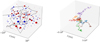 |
Fig. 1. (a) Schematic representation of the coherent current structures (CS) inside a zoomed view into the turbulent volume. The current filamentation creates a mixture of reconnecting (red) and non reconnecting (blue) current sheets. A particle executes a fractal random walk inside the turbulent volume. (b) Typical trajectories from our simulations for several particles, marked with different colors. The particles interact with an ensemble of CSs that form a fractal with dimension DF = 1.8 before they escape from the acceleration volume. |
The latter being distributed in such a way that they form a fractal set. Isliker & Vlahos (2003) analyzed this kind of random walk where particles move in a volume in which a fractal resides, usually traveling freely but being scattered when they encounter a part of the fractal set. They showed that in this case the distribution of free travel distances λsc in between two subsequent encounters with the fractal is distributed in good approximation according to
as long as DF < 2. For DF > 2, p(λsc) is decaying exponentially. Given that a dimension DF below 2 has been reported (Isliker & Vlahos 2003, McIntosh et al. 2002, Isliker et al. 2019), we are led to assume that p(λsc) is of power-law form, with index between –1 and –3. In Sioulas et al. (2020a), a parametric study of λscmin, λscmax has been performed, which indicates that the results are not sensitive to the precise values of the limits as long as the difference between the scales is several orders of magnitude. We were thus led to assume that the spatial separation of the scatterers ranges from λscmin = 102 cm to λscmax = 109 cm. The lower boundary represents the smaller-scale structures (i.e., 1 − 10 meters), while the higher limit is the characteristic scale of the acceleration volume. For the value of the fractal dimension we follow Isliker et al. (2019), using DF = 1.8, thus α = 1.2. Varying the fractal dimension in the range DF = 1.8 ± 0.2 has minimal effects for the steady state energy distributions.
As a result, the series of distances  , where i = 1, 2, ..., 106 is the particle index and j = 1, 2, ..., Ni the number of acceleration events for each particle, generated according to the probability density P(dr), characterizes the trajectory of the ith particle in space. However, since the particles travel in three dimensional space, we also have to generate a random number for the azimuthal angle ϕ, 0 < ϕ < 2π, and one for the polar angle θ through cos θ, −1 < cos θ < 1, which determine the direction of the particle motion. We can, therefore, monitor the coordinates of each particle, at the time of an energization event, according to
After a scattering event, which we consider here to be instantaneous, the particle’s energy changes by the amount of δW that is determined by the nature of the scatterer encountered. As a result, after the interaction, the particle i performs its jth spatial step of length  while having a constant velocity
  until the next encounter with a scatterer. Therefore, the time passed can be estimated by the free travel times. After a number of Ni encounters, the total time elapsed for the ith particle is
  We continue to monitor the particles’ energy and transport properties up to the final simulation time or until it crosses one of the box edges at time t = ti, esc. Typical random trajectories of particles from our simulations are shown in Fig. 1b. In order to keep track of the particles’ energy and spatial evolution, we monitor their properties at a number of logarithmically equi-spaced monitoring times tk, k = 0, 1, ..., K, with K typically chosen as 103 (see details in Sioulas et al. 2020b,a).
The environment that we model is similar to the one present in the lower solar corona. As a result, we impose a magnetic field of strength B = 100 G, an ambient temperature of T = 100 eV, and a plasma density of n0 = 109 cm−3. Finally, the Alfven speed VA is analogous to the electron thermal speed, attaining a value VA ∼ 7 × 108 cm s−1.
We focus our study on the random walk of ions and electrons in three different types of scatterers (1) reconnecting current sheets (Sect. 3.1), (2) non reconnecting current sheets (Sect. 3.2), and (3) synergy of reconnecting and non reconnecting current sheets (Sect. 3.3). The processes outlined here can be applied in several laboratory and astrophysical settings where strong turbulence and turbulent reconnection are driven.
3. Results
3.1. Systematic acceleration by reconnecting current sheets (RCSs).
We begin our analysis by considering an environment where all of the scatterers are modeled to behave as reconnecting current sheets (RCSs), systematically accelerating charged particles that travel in the turbulent volume. The energy gained after an interaction with a RCS is
(Isliker et al. 2017a). In our model, the magnetic fluctuation δB takes random values in the range δB ∈ [10−5G, 102G], obeying the probability density P(δB)∼δB−5/3 (Pisokas et al. 2018). As a result, the effective electric field  takes values in the range Eeff ∈ [2 ⋅ 10−7 statV/cm, 2 statV/cm]. Finally, we consider the effective length (ℓeff) to be a linear function of Eeff, ℓeff = aEeff + b, where the constants a, b can be estimated by limiting ℓeff to the range ℓeff ∈ [1 m, 1 km]. If we apply these values to Eq. (5), we can estimate that δW varies between 6 ⋅ 10−3 eV and 108 eV and follows a double power-law, see Fig. 2a (Isliker et al. 2017a; Pisokas et al. 2018). In energy space, the particle dynamics thus exhibit a systematic random walk, as only positive increments occur. In Fig. 2b, the distribution of the total number of acceleration events per particle is presented. The number of kicks ranges from 2 to 1055, with a mean of ∼72 acceleration events per particle. Following a scattering event, the ith particle departs from the scatterer with its renewed energy,
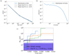 |
Fig. 2. (a) Distribution of energy increments δW for electrons interacting with RCSs. (b) Distribution of the number of energization events per electron. (c) Mean kinetic energy as a function of time, along with some typical electron trajectories marked with different colors. |
Here,  is given by Eq. (5), and j counts the number of energization events for the particle, up to a given time.
In Fig. 2c, we plot the evolution of the mean energy ⟨W(t)⟩ of the particles and the energy gain of a few typical particles along their trajectories. The mean energy initially increases exponentially in time, ⟨W(t)⟩ ∼ eaWt, and the acceleration time can be estimated from the relation tacc = 1/aw ∼ 0.09 s. The bulk of the particles gains only an almost negligible amount of energy from the interactions with the reconnecting current sheets. Only a small fraction of particles gains systematically energy, forming a power-law tail for energies Wkin > 1 keV, see Fig. 3. The interactions of particles with the scatterers pull particles from the thermal part of the distribution to super-thermal energies, resulting in a persisting tail (Fig. 3a). The bulk of the distribution basically remains unaffected and essentially is not heated by the presence of reconnecting current sheets.
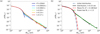 |
Fig. 3. (a) Temporal evolution of the kinetic energy distribution of the electrons in the presence of RCSs. (b) Kinetic energy distribution at t = 0 and t = 0.15 s (steady state) for the electrons remaining inside the volume with size L = 109 cm, together with a Maxwellian fit at low energies and a power-law fit at high energies. |
The evolution of the kinetic energy distribution in Fig. 3a indicates that the high-energy tail forms in a matter of a few milliseconds and persists even when more electrons have escaped from the volume, which in turn implies a very fast acceleration process. The distribution reaches its asymptotic state after a period of t ∼ 0.15 s, and the steady-state power-law tail yields an index k = 1.5, which is close to k = 1 + tacc/tesc ∼ 1.5, see Eq. (3), where tesc = 0.18 s, the median value of the times at which the electrons depart from the simulation volume.
The distribution of the particles’ escape time is shown in Fig. 4a. Taking into account the energy at which a particle leaves the box, denoted as Wesc, we show in Fig. 4b the escape energy distribution, which follows a scaling similar to that of the distribution of particles remaining inside the volume. Studying the escape time as a function of the escape energy of the particles, we conclude that the super-thermal particles (i.e., Wesc > 103 eV) tend to depart faster from the box in comparison to the low energy ones.
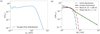 |
Fig. 4. (a) Escape time distribution. (b) Escape energy distribution of the electrons. |
In the following, the role of the simulation box’s length, as well as the magnetic fluctuations’ strength (δB) is examined. Keeping all the other parameters constant, we reduce the maximum value of the magnetic fluctuations’ strength to δB = 10G. As a result, δW takes values in the range [7 ⋅ 10−3 eV, 7 ⋅ 106 eV]. It turns out that the steady-state energy distribution is similar to the one in Fig. 3b, with the only difference being that the power-law tail is shorter and extends to a value that coincides with the maximum of δW ∼ 7 ⋅ 106 eV. This behavior (i.e., the distribution to preserve its shape with a tail that extends up to δWmax ) seems to hold in any of the cases tested. Also, other important parameters such as the escape and acceleration time do not seem to be considerably affected when reducing δB. Finally, in the case of RCSs, reducing the size of the simulation box, to still logical values, does not affect the shape of the steady-state energy distribution or the index of the power-law tail. As shown in Fig. 2, the probability density P(δW) follows a power-law scaling and extends over many orders of magnitude. Although the probability for a very efficient energization event that will result in a significant amount of energy gain is low, we always have a few particles accelerated to those high energies, even at the very first stages of the acceleration (i.e., t < 1 ms). As a result, the high-energy tail is always present. One other important observation is that there is a strong correlation between a significant energization event and the immediate departure of a particle from the acceleration volume.
Using the set of predefined monitoring times described above, we continue to keep track of the particle population properties up to the point where the majority of them has escaped, namely at time t = 1 s. A particle’s displacement from its initial position at time t = tn is  , and the mean square displacement for the ensemble of particles can be estimated through
To test the validity of the test-particle code, we first simulate an environment, in which a scattering event exclusively changes a particle’s direction of motion, leaving its energy constant (passive scatterers). In this case, we find that the diffusion of the charged particles is ballistic, with the power-law index holding a value of ∼2. This result is in good accordance with the results obtained by Isliker & Vlahos (2003) (as shown in Figs. 10 and 11 therein), where also the particles interact with passive scatterers that reside on a fractal with dimension DF < 2. Turning to active scatterers, the mean squared displacement is presented in Fig. 5a as a function of time. As one can observe, the charged particle diffusion is a two-stage process. For times up to t = 10−2 s we have an impulsive phase, which exhibits a ballistic scaling ⟨(Δr)2⟩∼t2.08. At larger times, the high-energy particles have departed from the volume and do not contribute any more to the statistics, which in turn leads to a reduction of the degree of super-diffusivity. As a result, for times greater than t = 10−2 s the power-law index decreases to αr = 1.52. In Fig. 5b, we have divided the particles into 50 logarithmically equi-spaced bins, according to the energy with which they escape the turbulent volume Wesc. As expected, the particles can be divided into three populations. The thermal particles (Wesc ≤ 103 eV) that with respect to their spatial diffusion properties behave similarly to particles interacting with passive scatterers, and the super-thermal particles, for which the spatial diffusion process is more efficient, with the power-law index linearly increasing from 2 to 2.45 and then saturating as the escape energy attains larger values.
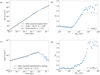 |
Fig. 5. (a) Spatial mean squared displacement as a function of time for the electrons interacting with RCSs. (b) Scaling index of the spatial mean squared displacement as a function of the escape energy. (c) Mean squared displacement in energy as a function of time for the electrons. (d) Scaling index of the mean squared displacement in energy as a function of the escape energy. |
The mean square displacement in energy can be estimated through
In Fig. 6c, we show the mean square displacement in energy as a function of time. It follows a power-law scaling of the form ⟨(ΔW)2⟩(t) = DW2taW2 with index, αw2 = 0.11, indicating a subdiffusive process in energy space. However, this result can be misleading. Similar to the spatial diffusion, if we divide the particles into logarithmically equi-spaced bins according to their escape energy, we find three distinct populations, see Fig. 6d. The bulk of the distribution consists of the thermal particles that diffuse in energy space in a subdiffusive manner, barely gaining energy before they escape from the simulation volume. On the other hand, a small fraction of the particles are accelerated to high energies (Wesc ≥ 103 eV), for which the energy transport process is very effective, as indicated by the power-law index that increases from 0.1 to 3.5 before it saturates for escape energies of very large values.
3.2. Ion acceleration by RCS’s.
Using the setup described in Sect. 3.1, we now replace the injected electron population with an equal number of ions (protons). Once again, the initial ensemble of the injected particles follows a Maxwellian distribution of temperature T = 100 eV. Since the energy increments δW do not depend on the mass of the particles, their distribution is identical to the one for electrons (Fig. 2a)). What changes, in this case, is the time between subsequent energization events. An exponential fit to the mean kinetic energy curve in Fig. 6 yields tacc = 0.98 s and shows that the energization process for protons is much slower than the one for electrons and is characterized by big time-gaps in-between scatterings with parts of the fractal. However, before escaping the acceleration volume, the protons are subjected on average to the same number of scattering events as the electrons.
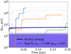 |
Fig. 6. Mean kinetic energy as a function of time, along with some typical proton trajectories marked with different colors. |
As shown in Fig. 7a, the power-law tail of the kinetic energy distribution is formed almost instantly (in a matter of a few milliseconds). However, it takes ∼1 s for the energy distribution to reach its steady state, which exhibits the same characteristics (i.e., minor heating accompanied by significant particle acceleration) as in the case of electrons. At t = 1 s (Fig. 7b), the lower energy part of the distribution can be fitted by a Maxwellian of temperature T = 132 eV, while for higher energies (Wkinet ≥ 103 eV) a power-law fit yields an index z = 1.5.
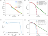 |
Fig. 7. (a) Temporal evolution of the kinetic energy distribution for protons. (b) Kinetic energy distribution at t = 0 and t = 1 s (steady state) for the protons remaining inside the box with size L = 109 cm, together with a Maxwellian fit at low energies and a power-law fit at high energies. (c) Escape time distribution for the protons. (d) Escape energy distribution for the protons, along with a power-law fit and a Maxwellian fit yielding a temperature T = 205 eV. |
In Fig. 7c, the distribution of the escape times for the protons is presented. The distribution remains uniform for escape times up to t ∼ 102 s and turns into a power-law with index z = 7.2 for larger escape times. The median value of the escape times is estimated as tesc ∼ 21.8 s. Keeping track of the energy at which each particle has escaped the acceleration volume as Wesc, we present in Fig. 7d the escape energy distribution. The low energy part of the distribution can be fitted by a Maxwellian of temperature T = 205 eV, while for escape energies greater than 103 eV a power-law tail of index z = 1.4 is formed.
Using binned statistics, we can determine the number of scatterings as a function of the escape energy. For the thermal particles (i.e., Wesc ≥ 102 eV), the escape energy is strongly influenced by the number of scatterings a particle is subjected to during the energization process. For higher escape energies, the functional form becomes, in approximation, a constant, attaining a value on the order of ∼100 scatterings per particle. The escape time is thus a function of the escape energy for the protons.
The mean squared displacement exhibits a power-law scaling ⟨(Δr)2⟩∼t2.06, which, after a time-span of t ∼ 0.1 s, decreases to t1.40, indicating a considerably less impulsive diffusion process than for electrons. This phase is also the longest-lasting one, as it persists for times up to t ∼ 100 s, the time where the majority of the particles have departed from the acceleration volume. Just like in the electron case, the change in the spatial diffusion behavior happens at the same time where the mean kinetic energy reaches its maximum value. Comparing the protons’ spatial diffusion to the electrons’ one, we can see that protons require a considerable amount of extra time in order to spread and escape the simulation box. This is reflected in both stages of diffusion, with the spatial diffusion scaling being characterized by smaller values of the power-law index ar. As a result, a significant increase in the escape time for the protons is observed when compared to the electrons.
3.3. Particle heating by nonreconnecting current sheets (CSs).
The main differences between reconnecting and non-reconnecting current sheets are (1) an encounter with the former results in systematic (i.e., δW is always positive), while with the latter in stochastic energy change. (2) The absence of reconnection, which would otherwise strongly enhance the effective electric field Eeff, results in a considerable reduction in the amount of energy change δW for the particles. Similar to the case of reconnecting current sheets, and according to the equation
the amount of energy change after an interaction with a non reconnecting CS is assumed to be
Depending on the particle velocity direction relative to the direction of the effective electric field, the encounter with a non reconnecting current sheet can either lead to energy gain or energy loss.
As a result, in order to model this stochastic accelerator, the knowledge of two probability density functions is required:
-
(1)
The probability density P(ℓeff) defines the effective acceleration lengths of the scatterers,
 . Here, ℓeff is assumed to follow a Kolmogorov spectrum, i.e.,
  , with the length of the scatterers taking values in the range ℓeff ∈ [1 m, 1 km], Zhdankin et al. (2013).
 -
(2)
The probability density P(Eeff) yields the effective electric field
 acting on the ith particle during its encounter with a non reconnecting CS, after it has performed its jth spatial step. In this case, since no respective studies suggesting the exact form of this PDF exists, we were obliged to study a multitude of different distributions.
We start our analysis assuming that P(Eeff) follows a narrow Gaussian distribution. As such, the effective electric field is almost constant across all of the scatterers in the turbulent volume, and what varies is each scatterer’s effective length. Another argument that satisfies this choice is its compatibility with the Central Limit Theorem (CLT). The effective electric field attached to each UCS can be thought of as the result of a plethora of small processes, a procedure that according to the CLT results in Gaussian distributions. We consider for the purposes of this study a Gaussian of mean μ = 103 ⋅ ED, and standard deviation σ = 10 ⋅ ED, where ED is the Dreicer field, ED ∼ 1.6 ⋅ 107 statV cm−1.
As a result of the selected PDF’s, the absolute values of δW are ranging between [3 eV, 8 ⋅ 103 eV] with a median value ∼1.6 ⋅ 101 eV, and their distribution forms a power-law, see Fig. 8a.
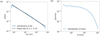 |
Fig. 8. (a) Distribution of the absolute values of the increments δW resulting from the Eq. (9), together with a power-law fit. (b) Distribution of the number of kicks per electron. |
We begin our analysis by uniformly inserting either a population of 106 electrons, or an equal number of ions (protons) inside the turbulent domain. The particles in their ensemble follow a Maxwellian distribution of temperature T = 100 eV. Following the setup of predefined monitoring times presented in Sect. 3.1, we keep track of the transport properties of the energized particles. During the acceleration process, each particle is subjected to many acceleration events (kicks), before it escapes the simulation box at time t = tesc, i.
Figure 8b exhibits the distribution of kicks per particle for the electrons. For the electron population, the mean value of the number of energization events is ∼94, with the number of kicks per particle ranging from 2 to 1232. The protons’ distribution of kicks per particle is very similar to the one of the electrons. The number of energization events per ion also has a wide range from 2 to 1167, with a mean value of ∼91 events.
Thus, in terms of acceleration events, the two particle populations behave in a very similar manner.
In Figs. 9a,c, we present the energization process for a number of selected electrons and ions, respectively. Apart from the stochastic nature of the acceleration process, what also becomes apparent is the fact that although ions attain approximately the same energies as the electrons, they require some tens of seconds more time inside the acceleration volume to do so. Figures 9b,d present the mean displacement in energy as function of time. Applying an exponential fit to the mean kinetic energy, one can estimate the acceleration time for each species, tacc = 1/aw, which is a good indicator of the rapidness of the acceleration process. We in this way estimate tacc ∼ 10 ssec for the electrons, and, tacc ∼ 200 s for the protons. Another timescale that differs between the two populations is the one that refers to the time they spend in the acceleration volume, tesc. In Figs. 10a,b, the distributions of the electron and proton escape times are presented. For the electrons, the distribution is in a good approximation uniform for times up to t ∼ 1 s and turns into a power-law with index z = 2.7 for larger times. The proton escape time distribution is of similar shape, namely uniform for times up to ∼90 s, followed by a steep power-law part with index z = 8.1. The median value of the electron escape time is estimated as tesc = 0.7 s, while for the protons as tesc = 26.9 s. The median escape times thus indicate that in general electrons tend to depart much faster from the acceleration volume than protons. It is important to note that the exact values of the escape and acceleration time strongly depend on the mean value of the imposed Gaussian distribution of the effective electric field. More specifically, increasing the distribution’s mean results in a reduction in both, the escape tesc and the acceleration tacc time, respectively.
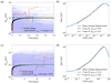 |
Fig. 9. (a) Mean kinetic energy as a function of time, and the energization process for several selected electrons. (b) Mean displacement in energy as a function of time for the electrons. (c) Mean kinetic energy as a function of time, and the energization process for a number of selected ions. (d) Mean displacement in energy as a function of time for the ions. |
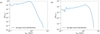 |
Fig. 10. (a) Distribution of the electrons’ escape time. (b) The distribution of the protons’ escape time. |
Figures 11a,b exhibit the mean squared displacement in space and in energy as a function of time for the electrons. They both attain a power-law scaling, the electrons are super-diffusive in position space with power-law index ar = 2.11, and they are clearly subdiffusive in energy space, with power-law index close to 0.25. Figures 11c,d give the mean square displacements in space and energy for the ions, and the ions show the same scaling indices as the electrons. What differs between the two populations is the time scale required for the ions to diffuse, which is, in general, an order of magnitude larger than the one required for the electrons. Taking a closer look at the initial phase of the energization process, one can see that the heavier ions need more time to gain energy and to efficiently begin diffusing in space. This observation is also in accordance with the fact that protons tend to stay longer inside the acceleration volume, resulting in a higher value for the escape time when compared to the electrons’ one.
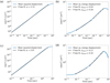 |
Fig. 11. (a) Spatial mean squared displacement as a function of time for the electrons. (b) Mean squared displacement in energy as a function of time for the electrons. (c) Spatial mean squared displacement as a function of time for the ions. (d) Mean squared displacement in energy as a function of time for the ions. |
The delayed response of the protons to the external fields is also apparent when considering the evolution of the kinetic energy distribution, see Figs. 12a,c. Although in the steady-state the electrons’ distribution does not have significant differences from the ions’ distribution, the time scales needed to attain this very similar energization state differ significantly.
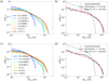 |
Fig. 12. (a) Evolution of the kinetic energy distribution for the electrons. (b) Electrons’ steady state distribution at time t = 0.5 s, along with a Maxwellian fit giving a temperature T = 2.61 keV. (c) Evolution of the kinetic energy distribution for the protons. (d) Protons’ steady state distribution at time t = 45 s, along with a Maxwellian fit giving a temperature T = 2.60 keV. |
Here, we have imposed a Gaussian distribution with mean μEeff = 103 ⋅ ED for the effective electric field Eeff, and the final kinetic energy distribution of both species in steady-state is close to a Maxwellian with temperature ∼2.6 KeV (see Figs. 12b,d), internally deformed to a power-law part, but no non-Maxwellian tail is developed. So the particles are only heated, and there is no acceleration. The question of course is how the mean and standard deviation of the electric field’s Gaussian distribution affect the steady-state kinetic energy distribution of the particles. A related parametric study presented in Figs. 13a,b revealed the following:
-
For any of the parameters tested, the steady-state distribution always is close to a Maxwellian (see Fig. 13a). This means that imposing an effective electric field that follows a Gaussian distribution leads to an energization mechanism able to drive the particle distribution to higher temperatures. The mechanism, however, fails to account for particle acceleration, as no power-law tails are formed.
-
As a result of increasing the mean of the Gaussian distribution to higher values, the kinetic energy distribution also attains higher temperatures, and the time needed to reach the steady-state is reduced (see Fig. 13b).
-
If the mean value of the Gaussian distribution is kept constant, but its standard deviation is reduced (i.e., the Gaussians become narrower), then the steady-state energy distribution fits better to a Maxwellian. In the limit where the Gaussian distribution is so narrow that it resembles a Delta function, the power-law part internal to the Maxwellian vanishes completely, and, depending on the mean of the imposed Gaussian, the kinetic energy distribution almost perfectly fits a Maxwellian.
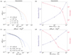 |
Fig. 13. (a) Steady-state kinetic energy distribution for different Gaussian distributions of Eeff. (b) Parametric study of (i) the temperature of the Maxwellian fit (blue), and (ii) the time required for the distribution to reach steady state (tacc; red) for Gaussian distributions of Eeff. (c) Steady-state kinetic energy distribution for different power-law distributions of Eeff. (d) Parametric study of (i) the temperature of the Maxwellian fit (blue), and (ii) the time required for the distribution to reach steady state (tacc; red) for power-law distributions of Eeff. In any case, the maximum value of Eeff is Emax = 102 ⋅ Emin. |
We have also performed a parametric study with a power-law distribution P(Eeff)∼E−5/3 for a number of lower (Emin) and upper (Emax) limits of the values of the electric field. In Figs. 13c,d, we show the effects of this study on the electron steady-state energy distribution. We can conclude:
-
Keeping the limits within a relatively small order of magnitude apart,
 , the steady-state distribution closely resembles a Maxwellian for all of the cases tested (see the parametric study in Fig. 13c).
 -
As a result of slightly adjusting the value of Emax to higher values, while keeping Emin constant, the steady-state energy distribution starts to diverge from a Maxwellian distribution, as a short and steep power-law tail forms on top of the thermalized part (not shown in Fig. 13c). Further increasing Emax results in a progressively softer power-law tail that extends to higher values in the energy domain. One has to keep in mind, however, the limitations imposed by the absence of reconnection on the physically attainable values of the electric field. It would be hard to imagine a too wide range in the values of electric fields in an environment dominated by non reconnecting CS.
-
Adjusting Emin to higher values drives the particle distribution to higher energies, reducing the time required to reach the steady-state (see Fig. 13d).
Overall, we can conclude that for a power-law distribution of Eeff, the minimum value Emin affects the thermalized part of the distribution, i.e., the steady state energy distribution becomes hotter for higher values of Emin. The shape of the distribution (i.e., how closely it resembles a Maxwellian) is determined by the ratio  . For αrange ∼ 102 the steady state distribution is closely related to a Maxwellian. For larger values of αrange the distribution starts to develop a power-law tail on top of the thermalized part, which gets increasingly softer as αrange increases.
3.4. Nonreconnecting CS’s as a possible coronal heating mechanism.
We have previously shown that stochastic energization of particles through non reconnecting CSs proves to be a mechanism that can effectively thermalize an injected particle distribution to increasingly high temperatures, depending on the mean value of the effective electric field imposed. The question, however, is wether or not this mechanism is able to drive a Maxwellian distribution of a typical chromospheric temperature of T = 104 K to the observed temperature of the solar corona of around T = 106 K. To answer this question, we reduce the initial temperature of the particles to T = 0.85 eV. We also reduce the mean value of the imposed electric field distribution to μEff = 102 ⋅ ED and the standard deviation to σEff = ED.
Otherwise, we keep the same setup as described in Sect. 3.3. In Figs. 14a,b we show the steady-state kinetic energy distribution for the electron and proton populations, respectively. In both cases the steady-state distribution very closely resembles a Maxwellian distribution of temperature T = 110 eV ∼ 106 K. What differs between the two populations is the time needed for the distribution to reach its steady-state, which is on the order of a few seconds for the electrons, while it is on the order of tens of seconds for the protons. Similar as in Sect. 3.3, if we increase the mean value of the Gaussian distribution of the effective electric field Eeff, higher temperatures are achieved in the final distribution, while, at the same time, a slight decrease in the acceleration time is observed.
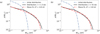 |
Fig. 14. Steady-state kinetic energy distribution for non-reconnecting CSs, where Eeff follows a Gaussian distribution of mean μ = 102 ⋅ ED and standard deviation σ = ED, (a) for electrons, (b) for protons, along with a Maxwellian fit of temperature T = 110 eV in both cases. |
3.5. Synergy of reconnecting and non-reconnecting CSs.
Following the model described in Sect. 2, we assume that the scatterers inside the turbulent volume are divided into two classes, reconnecting and non reconnecting CSs. A fraction P (0 ≤ P ≤ 1) are CSs, where the particles undergo stochastic acceleration, and the remaining fraction 1 − P are RCSs that give stochastic energy kicks to the particles. The nature of a scatterer is determined by drawing a random number α in the range Agudelo Rueda et al. (2021), and if α ≤ P we consider a non reconnecting CS, otherwise a RCS.
Regarding the characteristics of the non reconnecting CSs, we follow the setup presented in Sect. 3.3, and the statistical properties of the RCSs, as well as the characteristics of the acceleration volume, are kept as in Sect. 3.1. At time t = 0, a population of 106 particles is injected into the mixed environment. The injected distribution is a Maxwellian of temperature T = 100 eV. An extensive analysis has been performed for both electrons and ions, and the results presented here refer to electrons. The heating and acceleration characteristics of ions and electrons interacting with the mixed environment of scatterers are similar, the only difference being the time scales required to reach a steady state.
We first assume that P = 0.5, the probability to encounter a non reconnecting CS is equal to the probability of an encounter with a RCS. The effect of combining a stochastic energization mechanism (non reconnecting CSs) with a systematic one (RCSs) is presented in Fig. 15, where there is a combination of a classical random walk like behavior with sudden and often rather large increases in energy, i.e., a kind of strongly positively biased random walk.
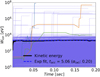 |
Fig. 15. Mean energy as a function of time, and energy of a few selected particles, marked by different colors. The particles undergo systematic and stochastic interactions with the CSs, with P = 0.5. |
Since the fraction of scatterers acting as reconnecting or non reconnecting current sheets in a turbulent environment cannot be expected to be always constant (for example, it can vary as the system evolves in time), it is important to understand how different combination ratios of reconnecting to non reconnecting CSs affect the energization process. Thereto, we start from the case P = 0, and we gradually increase the fraction of RCSs present in the system in our study.
When examining the steady-state kinetic energy distribution of the particles, we observe a significantly different behavior at the two ends of the spectrum, going from distributions of minor heating and extended power-law tails for P = 1 (i.e., only reconnecting RCSs are present in the system) to almost perfect Maxwellians of higher temperature without a tail for P = 0, see Fig. 16b. In Fig. 16a, we present the steady-state kinetic energy distribution for the particles that remain inside the turbulent volume at time t ∼ 0.8 s, along with the injected distribution, a Maxwellian fit, and a power-law fit, for P = 0.5. The energization process heats the low-energy particles, where the distribution follows a Maxwellian with a temperature T = 1 keV. In the high energy part of the distribution, a power-law tail is formed, which, in steady-state, has index k = 1.48 and extends from about 10 keV to 100 MeV. The power-law tail forms after a short period of a few milliseconds and persists even when more electrons have escaped from the acceleration volume. We can therefore conclude that a combination of the two kinds of scatterers changes the behavior of the turbulent volume from either a pure systematic accelerator or a pure efficient heating mechanism, for the values P = 1 or P = 0, respectively, to a combined and efficient heating and acceleration mechanism. Very similar behavior can be observed when studying the energy distribution of the escaping particles, as shown in Figs. 16c,d.
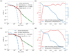 |
Fig. 16. (a) Steady-state kinetic energy distribution, along with a Maxwellian fit of temperature T ∼ 1 KeV and a power-law fit, for P = 0.5. (b) Power-law index of the steady-state kinetic energy distribution (blue), and the temperature of the Maxwellian fit (red), for different ratios P of the two kinds of scatterers. (c) Kinetic energy distribution for the escaped particles, for P = 0.5. (d) Power-law index of the kinetic energy distribution of the escaped particles (blue), and the temperature of the Maxwellian fit (red), for different ratios P of the two kinds of scatterers. |
Also important to note is the fact that as the percentage of RCSs present in the system increases, the acceleration time tacc, which is proportional to the time needed for the kinetic energy distribution to attain its asymptotic state, decreases (see Fig. 17). The opposite behavior is observed when considering the escape time of the particles, i.e., tesc increases as the percentage of RCSs increases (see Fig. 17).
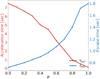 |
Fig. 17. Parametric study of (i) the escape time (tesc), and (ii) the acceleration time (tacc) for different ratios P of the two kinds of scatterers. |
In order to perform a study of the transport properties in space for the particle population, we once again make use of the set of predefined monitoring times described in Sect. 2. In Fig. 18, we show the spatial mean squared displacement as a function of time, which follows a power-law scaling with index k = 2.09 for P = 0.5. Also, the inset figure presents a parametric study for different ratios of reconnecting to non reconnecting CSs.
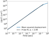 |
Fig. 18. Mean squared displacement as a function of time for P = 0.5. |
Important to note is the fact that for P ≥ 0.7, the diffusion process has two stages, showing a ballistic behavior for times up to t = 10−2 s with ar ranging in [2.06, 2.08], and a superdiffusive scaling for larger times with ar taking values in the range [1.53, 1.68] (similarly to Fig. 5a).
For values P ≤ 0.7, ar practically remains constant, ar ∼ 2.1, throughout the diffusion process.
4. Summary and conclusions
We have analyzed the energization of charged particles (electrons and protons) through their interaction with an environment of fractally distributed scatterers. The scatterers have been modeled to behave either as RCSs, or non reconnecting CSs. We have also tested a number of environments with the two energization mechanisms coexisting.
We have shown that the systematic interaction of particles with fractally distributed RCSs provides an efficient mechanism able to accelerate electrons and ions to very high energies, up to hundreds of MeV in a very short time. In the steady-state, the energy distributions exhibit very minor heating, and for energies, above 103 eV there always is a power-law tail of index z = 1.4 − 1.5 for the particles staying inside the acceleration volume, whereas the distributions of the escaping particles show a power-law tail with index ∼1.4. High energy particles undergo significant acceleration and easily depart from the energization volume. Their energy distribution is strongly correlated with the distribution of the energizations received from the RCSs. The extent of the power-law tail has been shown to be affected by the strength of the magnetic fluctuations (δB), and the maximum observed kinetic energy of the particles coincides with the maximum value of the energy increments δW, which are a function of δB. On the other hand, the kinetic energy distribution does not depend on the size of the simulation box. An analysis of the spatial transport properties for electrons interacting with RCS shows that spatial diffusion is a two-stage process. A ballistic phase during the first 10−2 s is followed by a less impulsive superdiffusive phase lasting at least up to ∼1 s.
Regarding the kinetic energy distribution, the results are identical for electrons and protons. What changes, however, is the increased time required for the protons to attain their steady-state distribution, as well as to spread through the simulation volume.
Replacing the scatterers with non reconnecting CSs, we have shown that stochastic energization by non reconnecting CS is a process that slowly but steadily heats particle distributions and increases their temperature, and it proves to be an efficient mechanism that can reproduce the heating of the Solar corona. The steady-state distribution’s temperature strongly depends on the mean value of the imposed electric field (μEeff). When μEeff increases, the steady-state distribution attains higher temperatures, while at the same time the acceleration time slightly decreases. Proton and electron distributions show similar behavior. Protons, though, require much more time to reach steady-state distributions. Particle transport in any case is superdiffusive in position space and subdiffusive in energy space. Based on the analysis presented in this article, we suggest that coronal heating is based on non reconnecting current sheets with a Gaussian distribution of the effective electric field of the CSs, which can be viewed, according to Einaudi et al. (2021), as another realization of the “nano-flares” model proposed by Parker (1983). We claim that “nanoflares” represent a small percentage of the CSs formed through the tangling of coronal magnetic field lines by the photospheric flows, whose signature possibly are the “campfires” recently observed by the Solar Orbiter mission (Berghmans et al. 2021; Chen et al. 2021b). We predict that when the density of “campfires” increases in the quiet corona, nonthermal particles will be present during coronal heating. Using a power-law distribution for the effective electric field Eeff, we reproduce the results obtained with the Gaussian distribution if arange = Emax/Emin is relatively small. For large values of arange, a very soft power-law tail appears in the energy distribution. Assuming that the non reconnecting CSs are associated with relatively weak electric fields, we can claim that they dominate the heating of the solar plasma independently of the probability distribution function of their effective electric field.
The effects of combining reconnecting with non reconnecting CSs in the same environment have also been investigated. A parametric study on P (i.e., the ratio of reconnecting to non reconnecting CSs) has shown that steady-state energy distributions generally consist of power-law tails for the high energy particles on top of a thermal part at low energies. The degree of the distribution’s heating, the extent and the index of the power-law tail, as well as the escape and the acceleration time, heavily depend on P. More specifically, when non reconnecting CSs dominate, the distributions are heated to high temperatures while the extent of the power-law tail gets shorter i.e., the tail begins at higher energies). For environments with larger P, where RCSs prevail, the steady-state distributions are characterized by minor heating and extended power-law tails of index z = 1.4 − 1.5. The escape and acceleration time depend on the fraction of the two types of scatterers. The higher the fraction of RCSs is, the larger is the escape time, while at the same time the smaller is the acceleration time for the particles.
How turbulent reconnection sets in in the solar corona depends on the large-scale MHD instabilities driven by the unstable magnetic topologies, for example, emerging magnetic flux, or kink instabilities. In most cases, a large-scale RCS sets in, which soon fragments, forming gradually a mixture of reconnecting and non reconnecting CSs. According to our analysis, the acceleration of high-energy electrons and ions dominates in the early phase when most CSs are still reconnecting, and then the gradual appearance of non reconnecting CSs will heat the plasma inside the turbulent reconnecting volume. On the other hand, the random shuffling of the magnetic fields that emerged from the turbulent convection zone or the emergence of small-scale magnetic loops drives easily non reconnecting CSs, which heat the solar corona and high energy particles are absent.
Therefore, the solar corona operates in two main modes. Explosive events start with reconnecting CSs and gradually end up with a mixture of reconnecting and non reconnecting CSs (based on our analysis, this can be achieved with a ratio P(t) varying in time). In the “quiet corona”, the random shuffling of the magnetic fields dominates the evolution of the coronal magnetic field, whereby non reconnecting CSs (elementary events Kanella & Gudiksen 2017, 2018; Einaudi et al. 2021) heat the solar atmosphere and drive the confined flares (Galsgaard & Nordlund 1996).
Our suggestions in this article depart from the currently very popular cartoon of the “standard flare scenario” and claim that each flare is a unique combination of non reconnecting and reconnecting CSs hosted in the 3D complex magnetic topology that is driven by convection zone turbulence. We cannot unravel all this complexity by analyzing an isolated RCS and without taking into account the presence of coherent structures in a turbulent environment that hosts RCSs and non reconnecting CSs.
The innovative parts of our work are (1) the use of a realistic 3D turbulent reconnection volume, with a fractal distribution of CSs, (2) the estimate of the energization and escape times inside the turbulent volume, (3) the investigation of the role of the systematic, the stochastic and the synergy of both energization mechanisms inside the turbulent reconnection volume, (4) the estimate of the energization (heating and acceleration) of electrons and ions, and their transport properties in energy and space. The weak points of our analysis are related to the fact that we use test particle simulations in steady-state turbulent reconnection environments, so the electromagnetic fields do not evolve in time and there is no feedback from the particles to the fields. At least a time-dependent evolution of the ratio of the RCSs (P(t)) would be needed to realistically explore the evolution of explosive events. Also, the statistical characteristics of the reconnecting and non reconnecting CSs are not known. We hope that the results from the Parker Solar Probe and future 3D MHD simulations, which follow the formation and evolution of turbulent reconnection volumes in time and space and incorporate the feedback from the kinetic evolution of the energetic particles in explosive and nonexplosive events, will clarify these issues soon.
Acknowledgments
We thank the anonymous referee for his comments and suggestions, which helped us to improve the article. Nikos Sioulas was supported by the HERMES DRIVE NASA Science Center grant No. 80NSSC20K0604.
References
- Agudelo Rueda, J. A., Verscharen, D., Wicks, R. T., et al. 2021, J. Plasma Phys., 87, 905870228 [CrossRef] [Google Scholar]
- Archontis, V., & Syntelis, P. 2019, Phil. Trans. R. Soc. A: Math. Phys. Eng. Sci., 377, 20180387 [CrossRef] [Google Scholar]
- Arnold, H., Drake, J. F., Swisdak, M., et al. 2021, Phys. Rev. Lett., 126, 135101 [NASA ADS] [CrossRef] [Google Scholar]
- Arzamasskiy, L., Kunz, M. W., Chandran, B. D. G., & Quataert, E. 2019, ApJ, 879, 53 [NASA ADS] [CrossRef] [Google Scholar]
- Arzner, K., Knaepen, B., Carati, D., Denewet, N., & Vlahos, L. 2006, AJ, 637, 322 [NASA ADS] [CrossRef] [Google Scholar]
- Arzner, K., & Vlahos, L. 2004, ApJ, 605, L69 [NASA ADS] [CrossRef] [Google Scholar]
- Berghmans, D., Auchère, F., Long, D. M., et al. 2021, A&A, 656, L4 [NASA ADS] [CrossRef] [EDP Sciences] [Google Scholar]
- Biskamp, D. 2000, Magnetic Reconnection in Plasmas, 3 [CrossRef] [Google Scholar]
- Biskamp, D. 2003, Magnetohydrodynamic Turbulence [Google Scholar]
- Boozer, A. H. 2019, Phys. Plasmas, 26, 082112 [CrossRef] [Google Scholar]
- Cargill, P., Vlahos, L., Baumann, G., Drake, J., & Nordlund, Å. 2012, Space Sci. Rev., 173, 223 [CrossRef] [Google Scholar]
- Cassak, P. A., & Fuselier, S. A. 2016, in Reconnection at Earth’s Dayside Magnetopause, eds. W. Gonzalez, & E. Parker, 427, 213 [CrossRef] [Google Scholar]
- Che, H., & Zank, G. P. 2019, J. Phys. Conf. Ser., 1332, 012003 [NASA ADS] [CrossRef] [Google Scholar]
- Chen, B., Battaglia, M., Krucker, S., Reeves, K. K., & Glesener, L. 2021a, ApJ, 908, L55 [CrossRef] [Google Scholar]
- Chen, Y., Przybylski, D., Peter, H., & Tian, H. 2021b, EGU General Assembly Conference Abstracts, 5061, EGU21 [Google Scholar]
- Cheng, X., Li, Y., Wan, L. F., et al. 2018, ApJ, 866, 64 [Google Scholar]
- Chitta, L. P., & Lazarian, A. 2020, ApJ, 890, L2 [Google Scholar]
- Chitta, L. P., Peter, H., Priest, E. R., & Solanki, S. K. 2020, A&A, 644, A130 [EDP Sciences] [Google Scholar]
- Comisso, L., & Sironi, L. 2019, ApJ, 886, 122 [Google Scholar]
- Coppi, B., Laval, G., & Pellat, R. 1966, Phys. Rev. Lett., 16, 1207 [NASA ADS] [CrossRef] [Google Scholar]
- Dahlburg, R. B., Einaudi, G., Taylor, B. D., et al. 2016, ApJ, 817, 47 [NASA ADS] [CrossRef] [Google Scholar]
- Dahlin, J. T. 2020, Phys. Plasmas, 27, 100601 [CrossRef] [Google Scholar]
- Dahlin, J. T., Drake, J. F., & Swisdak, M. 2017, Phys. Plasmas, 24, 092110 [Google Scholar]
- Dimitropoulou, M., Isliker, H., Vlahos, L., & Georgoulis, M. K. 2013, A&A, 553, A65 [NASA ADS] [CrossRef] [EDP Sciences] [Google Scholar]
- Dmitruk, P., Matthaeus, W. H., & Seenu, N. 2004, AJ, 617, 667 [NASA ADS] [CrossRef] [Google Scholar]
- Drake, J., & Swisdak, M. 2014, APS Meeting Abstracts, 2014, TO7.014 [Google Scholar]
- Drake, J. F., Swisdak, M., Che, H., & Shay, M. A. 2006, Nature, 443, 553 [Google Scholar]
- Einaudi, G., Dahlburg, R. B., Ugarte-Urra, I., et al. 2021, ApJ, 910, 84 [NASA ADS] [CrossRef] [Google Scholar]
- Fermi, E. 1949, Phys. Rev., 75, 1169 [NASA ADS] [CrossRef] [Google Scholar]
- Fermi, E. 1954, AJ, 119, 1 [NASA ADS] [CrossRef] [Google Scholar]
- Galsgaard, K., & Nordlund, Å. 1996, J. Geophys. Res., 101, 13445 [NASA ADS] [CrossRef] [Google Scholar]
- Galsgaard, K., & Nordlund, Å. 1997a, J. Geophys. Res., 102, 219 [CrossRef] [Google Scholar]
- Galsgaard, K., & Nordlund, Å. 1997b, J. Geophys. Res., 102, 231 [NASA ADS] [CrossRef] [Google Scholar]
- Hudson, H. S., Simões, P. J. A., Fletcher, L., Hayes, L. A., & Hannah, I. G. 2021, MNRAS, 501, 1273 [Google Scholar]
- Inoue, S., Shiota, D., Bamba, Y., & Park, S.-H. 2018, ApJ, 867, 83 [CrossRef] [Google Scholar]
- Isliker, H., & Vlahos, L. 2003, Phys. Rev. E, 67, 026413 [NASA ADS] [CrossRef] [Google Scholar]
- Isliker, H., Pisokas, T., Vlahos, L., & Anastasiadis, A. 2017a, ApJ, 849, 35 [NASA ADS] [CrossRef] [Google Scholar]
- Isliker, H., Vlahos, L., & Constantinescu, D. 2017b, Phys. Rev. Lett., 119, 045101 [NASA ADS] [CrossRef] [Google Scholar]
- Isliker, H., Archontis, V., & Vlahos, L. 2019, AJ, 882, 57 [CrossRef] [Google Scholar]
- Jiang, C., Wu, S. T., Feng, X., & Hu, Q. 2016, Nat. Commun., 7, 11522 [NASA ADS] [CrossRef] [Google Scholar]
- Kanella, C., & Gudiksen, B. V. 2017, A&A, 603, A83 [NASA ADS] [CrossRef] [EDP Sciences] [Google Scholar]
- Kanella, C., & Gudiksen, B. V. 2018, A&A, 617, A50 [NASA ADS] [CrossRef] [EDP Sciences] [Google Scholar]
- Karimabadi, H., & Lazarian, A. 2013, Phys. Plasmas, 20, 112102 [NASA ADS] [CrossRef] [Google Scholar]
- Karimabadi, H., Roytershteyn, V., Daughton, W., & Liu, Y.-H. 2013a, Space Sci. Rev., 178, 307 [CrossRef] [Google Scholar]
- Karimabadi, H., Roytershteyn, V., Wan, M., et al. 2013b, Phys. Plasmas, 20, 012303 [Google Scholar]
- Karimabadi, H., Roytershteyn, V., Vu, H. X., et al. 2014, Phys. Plasmas, 21, 062308 [NASA ADS] [CrossRef] [Google Scholar]
- Knizhnik, K., Swisdak, M., & Drake, J. F. 2011, ApJ, 743, L35 [NASA ADS] [CrossRef] [Google Scholar]
- Kowal, G., Lazarian, A., Vishniac, E. T., & Otmianowska-Mazur, K. 2009, ApJ, 700, 63 [Google Scholar]
- Kowal, G., Falceta-Gonçalves, D. A., Lazarian, A., & Vishniac, E. T. 2017, ApJ, 838, 91 [NASA ADS] [CrossRef] [Google Scholar]
- Kozak, L. V., Petrenko, B. A., Lui, A. T. Y., et al. 2018, Ann. Geophys., 36, 1303 [NASA ADS] [CrossRef] [Google Scholar]
- Kumar, R., Eichler, D., Gaspari, M., & Spitkovsky, A. 2017, ApJ, 835, 295 [NASA ADS] [CrossRef] [Google Scholar]
- Lazarian, A., & Vishniac, E. T. 1999, AJ, 517, 700 [NASA ADS] [CrossRef] [Google Scholar]
- Lazarian, A., Vlahos, L., Kowal, G., et al. 2012, Space Sci. Rev., 173, 557 [Google Scholar]
- Lazarian, A., Eyink, G. L., Jafari, A., et al. 2020, Phys. Plasmas, 27, 012305 [NASA ADS] [CrossRef] [Google Scholar]
- Leake, J. E., Daldorff, L. K. S., & Klimchuk, J. A. 2020, ApJ, 891, 62 [NASA ADS] [CrossRef] [Google Scholar]
- Leonardis, E., Chapman, S. C., Daughton, W., Roytershteyn, V., & Karimabadi, H. 2013, Phys. Rev. Lett., 110, 205002 [NASA ADS] [CrossRef] [Google Scholar]
- Li, X., Guo, F., Li, H., Stanier, A., & Kilian, P. 2019, ApJ, 884, 118 [Google Scholar]
- Liang, J., Lin, Y., Johnson, J. R., Wang, Z.-X., & Wang, X. 2017, Phys. Plasmas, 24, 102110 [NASA ADS] [CrossRef] [Google Scholar]
- Lin, R. P., Krucker, S., Hurford, G. J., et al. 2003, ApJ, 595, L69 [NASA ADS] [CrossRef] [Google Scholar]
- Longair, M. S. 2011, High Energy Astrophysics (Cambridge: Cambridge University Press) [Google Scholar]
- Loureiro, N. F., & Uzdensky, D. A. 2016, Plasma Phys. Controlled Fusion, 58, 014021 [NASA ADS] [CrossRef] [Google Scholar]
- Lu, S., Wang, R., Lu, Q., et al. 2020, Nat. Commun., 11, 5049 [NASA ADS] [CrossRef] [Google Scholar]
- Matthaeus, W. H., & Lamkin, S. L. 1986, Phys. Fluids, 29, 2513 [Google Scholar]
- Matthaeus, W. H., & Velli, M. 2011, Space Sci. Rev., 160, 145 [Google Scholar]
- McIntosh, S. W., Charbonneau, P., Bogdan, T. J., Liu, H.-L., & Norman, J. P. 2002, Phys. Rev. E, 65, 046125 [NASA ADS] [CrossRef] [Google Scholar]
- Müller, D., St. Cyr, O. C., Zouganelis, I., et al. 2020, A&A, 642, A1 [Google Scholar]
- Oishi, J. S., Mac Low, M.-M., Collins, D. C., & Tamura, M. 2015, ApJ, 806, L12 [NASA ADS] [CrossRef] [Google Scholar]
- Onofri, M., Primavera, L., Malara, F., & Veltri, P. 2004, Phys. Plasmas, 11, 4837 [NASA ADS] [CrossRef] [Google Scholar]
- Onofri, M., Isliker, H., & Vlahos, L. 2006, Phys. Rev. Lett., 96, 151102 [CrossRef] [Google Scholar]
- Osman, K. T., Matthaeus, W. H., Gosling, J. T., et al. 2014, Phys. Rev. Lett., 112, 215002 [NASA ADS] [CrossRef] [Google Scholar]
- Parker, E. N. 1957, J. Geophys. Res., 62, 509 [Google Scholar]
- Parker, E. N. 1983, AJ, 264, 635 [NASA ADS] [CrossRef] [Google Scholar]
- Parnell, C. E., Maclean, R. C., Haynes, A. L., & Galsgaard, K. 2011, in Astrophysical Dynamics: From Stars to Galaxies, eds. N. H. Brummell, A. S. Brun, M. S. Miesch, & Y. Ponty, 271, 227 [NASA ADS] [Google Scholar]
- Petschek, H. E. 1964, Magnetic Field Annihilation, 50, 425 [Google Scholar]
- Phan, T. D., Bale, S. D., Eastwood, J. P., et al. 2020, ApJS, 246, 34 [Google Scholar]
- Pisokas, T., Vlahos, L., & Isliker, H. 2018, AJ, 852, 64 [NASA ADS] [CrossRef] [Google Scholar]
- Pisokas, T., Vlahos, L., Isliker, H., Tsiolis, V., & Anastasiadis, A. 2017, AJ, 835, 214 [NASA ADS] [CrossRef] [Google Scholar]
- Rappazzo, A. F., Velli, M., & Einaudi, G. 2010, ApJ, 722, 65 [NASA ADS] [CrossRef] [Google Scholar]
- Rappazzo, A. F., Velli, M., & Einaudi, G. 2013, ApJ, 771, 76 [NASA ADS] [CrossRef] [Google Scholar]
- Schaffner, D. A., & Brown, M. R. 2015, ApJ, 811, 61 [NASA ADS] [CrossRef] [Google Scholar]
- Shibata, K., & Tanuma, S. 2001, Earth. Planets, and Space, 53, 473 [CrossRef] [Google Scholar]
- Shivamoggi, B. K. 1997, Ann. Phys., 253, 239 [NASA ADS] [CrossRef] [Google Scholar]
- Sioulas, N., Isliker, H., & Vlahos, L. 2020a, ApJ, 895, L14 [NASA ADS] [CrossRef] [Google Scholar]
- Sioulas, N., Isliker, H., Vlahos, L., Koumtzis, A., & Pisokas, T. 2020b, MNRAS, 491, 3860 [NASA ADS] [CrossRef] [Google Scholar]
- Sitnov, M., Birn, J., Ferdousi, B., et al. 2019, Space Sci. Rev., 215, 31 [CrossRef] [Google Scholar]
- Tu, C. Y., & Marsch, E. 1995, Space Sci. Rev., 73, 1 [Google Scholar]
- Turkmani, R., Vlahos, L., Galsgaard, K., Cargill, P., & Isliker, H. 2005, ApJ, 620, L59 [CrossRef] [Google Scholar]
- Vlahos, L., & Isliker, H. 2019, Plasma Phys. Controlled Fusion, 61, 014020 [NASA ADS] [CrossRef] [Google Scholar]
- Vlahos, L., Isliker, H., & Lepreti, F. 2004, AJ, 608, 540 [NASA ADS] [CrossRef] [Google Scholar]
- Vlahos, L., Isliker, H., Kominis, Y., & Hizanidis, K. 2008, ArXiv e-prints [arXiv:0805.0419] [Google Scholar]
- Vlahos, L., Pisokas, T., Isliker, H., Tsiolis, V., & Anastasiadis, A. 2016, AJ, 827, L3 [NASA ADS] [CrossRef] [Google Scholar]
- Wang, S., & Yokoyama, T. 2019, Phys. Plasmas, 26, 072109 [NASA ADS] [CrossRef] [Google Scholar]
- Zhdankin, V., Uzdensky, D. A., Perez, J. C., & Boldyrev, S. 2013, AJ, 771, 124 [CrossRef] [Google Scholar]
- Zweibel, E. G., & Yamada, M. 2016, Proc. R. Soc. London, Ser. A, 472, 20160479 [Google Scholar]
All Figures
|
Fig. 1. (a) Schematic representation of the coherent current structures (CS) inside a zoomed view into the turbulent volume. The current filamentation creates a mixture of reconnecting (red) and non reconnecting (blue) current sheets. A particle executes a fractal random walk inside the turbulent volume. (b) Typical trajectories from our simulations for several particles, marked with different colors. The particles interact with an ensemble of CSs that form a fractal with dimension DF = 1.8 before they escape from the acceleration volume. |
| In the text | |
|
Fig. 2. (a) Distribution of energy increments δW for electrons interacting with RCSs. (b) Distribution of the number of energization events per electron. (c) Mean kinetic energy as a function of time, along with some typical electron trajectories marked with different colors. |
| In the text | |
|
Fig. 3. (a) Temporal evolution of the kinetic energy distribution of the electrons in the presence of RCSs. (b) Kinetic energy distribution at t = 0 and t = 0.15 s (steady state) for the electrons remaining inside the volume with size L = 109 cm, together with a Maxwellian fit at low energies and a power-law fit at high energies. |
| In the text | |
|
Fig. 4. (a) Escape time distribution. (b) Escape energy distribution of the electrons. |
| In the text | |
|
Fig. 5. (a) Spatial mean squared displacement as a function of time for the electrons interacting with RCSs. (b) Scaling index of the spatial mean squared displacement as a function of the escape energy. (c) Mean squared displacement in energy as a function of time for the electrons. (d) Scaling index of the mean squared displacement in energy as a function of the escape energy. |
| In the text | |
|
Fig. 6. Mean kinetic energy as a function of time, along with some typical proton trajectories marked with different colors. |
| In the text | |
|
Fig. 7. (a) Temporal evolution of the kinetic energy distribution for protons. (b) Kinetic energy distribution at t = 0 and t = 1 s (steady state) for the protons remaining inside the box with size L = 109 cm, together with a Maxwellian fit at low energies and a power-law fit at high energies. (c) Escape time distribution for the protons. (d) Escape energy distribution for the protons, along with a power-law fit and a Maxwellian fit yielding a temperature T = 205 eV. |
| In the text | |
|
Fig. 8. (a) Distribution of the absolute values of the increments δW resulting from the Eq. (9), together with a power-law fit. (b) Distribution of the number of kicks per electron. |
| In the text | |
|
Fig. 9. (a) Mean kinetic energy as a function of time, and the energization process for several selected electrons. (b) Mean displacement in energy as a function of time for the electrons. (c) Mean kinetic energy as a function of time, and the energization process for a number of selected ions. (d) Mean displacement in energy as a function of time for the ions. |
| In the text | |
|
Fig. 10. (a) Distribution of the electrons’ escape time. (b) The distribution of the protons’ escape time. |
| In the text | |
|
Fig. 11. (a) Spatial mean squared displacement as a function of time for the electrons. (b) Mean squared displacement in energy as a function of time for the electrons. (c) Spatial mean squared displacement as a function of time for the ions. (d) Mean squared displacement in energy as a function of time for the ions. |
| In the text | |
|
Fig. 12. (a) Evolution of the kinetic energy distribution for the electrons. (b) Electrons’ steady state distribution at time t = 0.5 s, along with a Maxwellian fit giving a temperature T = 2.61 keV. (c) Evolution of the kinetic energy distribution for the protons. (d) Protons’ steady state distribution at time t = 45 s, along with a Maxwellian fit giving a temperature T = 2.60 keV. |
| In the text | |
|
Fig. 13. (a) Steady-state kinetic energy distribution for different Gaussian distributions of Eeff. (b) Parametric study of (i) the temperature of the Maxwellian fit (blue), and (ii) the time required for the distribution to reach steady state (tacc; red) for Gaussian distributions of Eeff. (c) Steady-state kinetic energy distribution for different power-law distributions of Eeff. (d) Parametric study of (i) the temperature of the Maxwellian fit (blue), and (ii) the time required for the distribution to reach steady state (tacc; red) for power-law distributions of Eeff. In any case, the maximum value of Eeff is Emax = 102 ⋅ Emin. |
| In the text | |
|
Fig. 14. Steady-state kinetic energy distribution for non-reconnecting CSs, where Eeff follows a Gaussian distribution of mean μ = 102 ⋅ ED and standard deviation σ = ED, (a) for electrons, (b) for protons, along with a Maxwellian fit of temperature T = 110 eV in both cases. |
| In the text | |
|
Fig. 15. Mean energy as a function of time, and energy of a few selected particles, marked by different colors. The particles undergo systematic and stochastic interactions with the CSs, with P = 0.5. |
| In the text | |
|
Fig. 16. (a) Steady-state kinetic energy distribution, along with a Maxwellian fit of temperature T ∼ 1 KeV and a power-law fit, for P = 0.5. (b) Power-law index of the steady-state kinetic energy distribution (blue), and the temperature of the Maxwellian fit (red), for different ratios P of the two kinds of scatterers. (c) Kinetic energy distribution for the escaped particles, for P = 0.5. (d) Power-law index of the kinetic energy distribution of the escaped particles (blue), and the temperature of the Maxwellian fit (red), for different ratios P of the two kinds of scatterers. |
| In the text | |
|
Fig. 17. Parametric study of (i) the escape time (tesc), and (ii) the acceleration time (tacc) for different ratios P of the two kinds of scatterers. |
| In the text | |
|
Fig. 18. Mean squared displacement as a function of time for P = 0.5. |
| In the text | |
Current usage metrics show cumulative count of Article Views (full-text article views including HTML views, PDF and ePub downloads, according to the available data) and Abstracts Views on Vision4Press platform.
Data correspond to usage on the plateform after 2015. The current usage metrics is available 48-96 hours after online publication and is updated daily on week days.
Initial download of the metrics may take a while.