| Issue |
A&A
Volume 657, January 2022
|
|
|---|---|---|
| Article Number | A4 | |
| Number of page(s) | 15 | |
| Section | Stellar structure and evolution | |
| DOI | https://doi.org/10.1051/0004-6361/202040062 | |
| Published online | 20 December 2021 | |
Multiplicity of Galactic luminous blue variable stars⋆,⋆⋆
1
Royal Observatory of Belgium, Avenue Circulaire/Ringlaan 3, 1180 Brussels, Belgium
e-mail: This email address is being protected from spambots. You need JavaScript enabled to view it.
2
Institute of Astronomy, KU Leuven, Celestijnenlaan 200D, 3001 Leuven, Belgium
3
The CHARA Array of Georgia State University, Mount Wilson Observatory, Mount Wilson, CA 91023, USA
4
Research Director F.R.S.-FNRS, Space Sciences, Technologies and Astrophysics Research (STAR) Institute, Université de Liège, Allée du 6 Août, 19c, Bât B5c, 4000 Liège, Belgium
5
South African Astronomical Observatory, PO Box 9 Observatory 7935, South Africa
6
Australian Astronomical Optics – Macquarie, Faculty of Science and Engineering, Macquarie University, North Ryde, NSW 2113, Australia
Received:
4
December
2020
Accepted:
4
October
2021
Abstract
Context. Luminous blue variables (LBVs) are characterised by strong photometric and spectroscopic variability. They are thought to be in a transitory phase between O-type stars on the main sequence and the Wolf-Rayet stage. Recent studies also evoked the possibility that they might be formed through binary interaction. Only a few are known in binary systems so far, but their multiplicity fraction is still uncertain.
Aims. We derive the binary fraction of the Galactic LBV population. We combine multi-epoch spectroscopy and long-baseline interferometry to probe separations from 0.1 to 120 mas around confirmed and candidate LBVs.
Methods. We used a cross-correlation technique to measure the radial velocities of these objects. We identified spectroscopic binaries through significant radial velocity variability with an amplitude larger than 35 km s−1. We also investigated the observational biases to take them into account when we established the intrinsic binary fraction. We used CANDID to detect interferometric companions, derive their flux fractions, and their positions on the sky.
Results. From the multi-epoch spectroscopy, we derive an observed spectroscopic binary fraction of 26−10+16%. Considering period and mass ratio ranges from log(Porb) = 0 − 3 (i.e. from 1 to 1000 days), q = 0.1 − 1.0, and a representative set of orbital parameter distributions, we find a bias-corrected binary fraction of 62−24+38%. Based on data of the interferometric campaign, we detect a binary fraction of 70 ± 9% at projected separations between 1 and 120 mas. Based on the derived primary diameters and considering the distances of these objects, we measure for the first time the exact radii of Galactic LBVs to be between 100 and 650 R⊙. This means that it is unlikely that short-period systems are included among LBV-like stars.
Conclusions. This analysis shows for the first time that the binary fraction in the Galactic LBV population is large. If they form through single-star evolution, their orbit must be large initially. If they form through a binary channel, the implication is that either massive stars in short binary systems must undergo a phase of fully non-conservative mass transfer to be able to sufficiently widen the orbit to form an LBV, or that LBVs form through merging in initially binary or triple systems. Interferometric follow-up would provide the distributions of orbital parameters at more advanced stages and would serve to quantitatively test the binary evolution in massive stars.
Key words: stars: variables: S Doradus / stars: evolution / binaries: general / stars: massive
Full Table A.1 is only available at the CDS via anonymous ftp to cdsarc.u-strasbg.fr (130.79.128.5) or via http://cdsarc.u-strasbg.fr/viz-bin/cat/J/A+A/657/A4
Based on observations collected at the ESO Paranal observatory under ESO program 0102.D-0460(A), on spectra obtained with the Mercator Telescope, operated on the island of La Palma by the Flemish Community, at the Spanish Observatorio del Roque de los Muchachos of the Instituto de Astrofísica de Canarias, on observations made with the Southern African Large Telescope (SALT) under programme 2019-1-SCI-001, and with the TIGRE telescope, located at La Luz observatory, Mexico (TIGRE is a collaboration of the Hamburger Sternwarte, the Universities of Hamburg, Guanajuato, and Liège).
© ESO 2021
1. Introduction
Luminous blue variables (LBV) are enigmatic objects located in the upper part of the Hertzsprung-Russell diagram (HRD). They have long been considered to be a brief evolutionary phase describing massive stars in transition to the Wolf-Rayet (WR) phase (Lamers & Nugis 2002). Although O and WR stars have high mass-loss rates, when integrated over the stellar lifetime, these rates are usually not sufficient to enable a smooth direct evolution. At some point in their past, the progenitors of WR stars must have undergone a phase of extreme mass loss, during which their outer envelopes were removed to reveal the bare core that became the WR star. This extreme mass loss is thought to occur either during a red supergiant or an LBV phase (Maeder & Meynet 2000).
However, this traditional view of LBVs as single-star evolutionary phase was strongly questioned (Gallagher 1989). Theory (Groh et al. 2013) and observations (see e.g. Gal-Yam et al. 2007; Kiewe et al. 2012) showed that some progenitors of core-collapse supernovae (CCSNe, especially type IIn) appear to be LBVs, while theoretically, the latest stage before exploding as CCSNe was expected to be either the red supergiant (RSG), blue supergiant, or WR stage. This significantly draws the hypothesis into doubt that LBVs are massive stars in transition to core He-burning objects. Recently, the relative isolation of LBVs was the subject of a lively debate (Smith & Tombleson 2015; Smith 2016, 2019; Humphreys et al. 2016; Davidson et al. 2016; Aghakhanloo et al. 2017; Aadland et al. 2018). According to Smith & Tombleson (2015), when the population of LBVs is compared with populations of O- or WR-type stars, the relative isolation of LBVs suggests that it is unlikely that their population turns into the observed population of WR stars. These authors suggested that LBVs are not concentrated in young massive clusters with early O-type stars, as would be expected from single-star evolution. Rather, LBVs would be largely products of binary or multiple systems that would have been kicked far from their birth places by an explosion of their companions. This binary product scenario has been proposed before by Justham et al. (2014), in which an early case B accretion (soon after the core H-burning phases) could allow the massive star to gain sufficient mass to reach core collapse with the properties expected for an LBV (spun up, chemically enriched, and rejuvenated).
The evolutionary origin of LBVs is thus still an open question in modern astrophysics. We know about LBVs that they are massive, hot stars with very high mass-loss rates, located near the Eddington limit. The only way to classify a star as an LBV is by studying its variability (Weis & Bomans 2020), either photometrically or spectroscopically. To be classified as a classical LBV, a star must undergo S-Doradus (hereafter S-Dor) cycles, which are temperature changes at practically constant luminosity (Humphreys & Davidson 1994; Groh et al. 2009a; Smith 2017), or giant eruptions. The S-Dor cycle consists of two different phases of variability: (1) a cool phase caused by its atmosphere that develops through optically thick winds, exhibiting spectra that look like those of A- or F-type stars, and (2) a quiescence phase during which the star has features similar to those of early B or O supergiant or even WR stars. The true mechanism that produces S-Dor cycles still remains uncertain, even though several hypotheses have been developed to explain this variability, such as proximity of the Eddington limit, pulsations, binarity, turbulent pressure and sub-surface convection, and wind-envelope interaction (see Humphreys & Davidson 1994 and references therein, Gräfener et al. 2012; Sanyal et al. 2015; Grassitelli et al. 2021, among others).
Some stars also present common characteristics with the classical LBVs, but have never been detected to show S-Dor variability or giant eruption: the dormant or candidate LBVs (Humphreys & Davidson 1994). These stars are also located close to the Humphreys-Davidson limit in the upper part of the HRD. We refer to the confirmed and candidate LBVs with the general term LBV-like objects.
The most frequently studied star in this LBV-like class of object, η Car, was thought to be the result of a merging induced by three stars that expelled the original primary star and caused the great eruption observed in the 1800s (Portegies Zwart & van den Heuvel 2016; Smith et al. 2018). Since η Car was detected to be a binary, other LBVs and LBV-like objects were identified as binary systems: HD 5980 (Koenigsberger et al. 2010) in the Small Magellanic Cloud, HDE 269128 in the Large Magellanic Cloud, HR Car (Boffin et al. 2016), HD 326823 (Richardson et al. 2011), the Pistol star (Martayan et al. 2012), and MWC 314 (Lobel et al. 2013), all located in the Milky Way. Despite these discoveries, the binary fraction in the population of LBV-like objects has not yet been unveiled. Through their X-ray survey, Nazé et al. (2012) detected four objects (η Car, Schulte 12, GAL 026.47+00.02, and Cl* Westerlund 1 W 243) for which the X-ray detections are reminiscent of wind-wind collisions in binary systems, and five objects (P Cyg, AG Car, HD 160529, HD 316285, and Sher 25) in which the X-ray detections reach a strong limit that can be due to binarity, among other explanations. The authors concluded from half of the sample of Galactic LBV-like objects that the binary fraction must be between 26% and 69%. Martayan et al. (2016) investigated the environments that surround seven LBV-like stars and searched for possible wide-orbit companions. From infrared images, they found that two out of seven objects (HD 168625 and MWC 314) might be wide-orbit binaries, deducing from low-number statistics that about 30% of LBV-like stars are in binary systems.
Assuming that the LBV phase is a transition phase between the O and WR stages, we would expect that more objects are in binary systems. It is indeed quite surprising that more than 70% of the O-type stars (Sana et al. 2012, 2014; Moe & Di Stefano 2017), 40% of the Be stars (Oudmaijer & Parr 2010), and over 50% of the WRs (van der Hucht 2001; Dsilva et al. 2020) are detected to be part of multiple systems, whilst the binarity of the LBV-like objects is expected to be approximately 30%. The detection of gravitationally bound companions is difficult through spectroscopy because of (1) the difference in luminosity between the components and (2) the strong variability characterising the LBV-like stars (as Weis & Bomans 2020 mentioned in their review). We propose to combine spectroscopy and interferometry to study the multiplicity properties of a sample of Galactic confirmed and candidate LBVs using multi-epoch and multi-instrument observations. The paper is organised as follows. Section 2 describes the sample, the multi-epoch and multi-instrument observations, and their reduction. The spectroscopic observations are analysed in Sect. 3. Section 4 presents the interferometric detections. Finally, Sect. 5 discusses the effect of the overall binary fraction on the evolutionary nature of the LBVs, and the conclusions are given in Sect. 6.
2. Sample, observations, and data reduction
2.1. Sample
We built our sample from the LBV catalogues of Clark et al. (2005) and Nazé et al. (2012). The spectroscopic and interferometric samples are different because the instrumental and observational constraints are different.
The spectroscopic sample gathers all the Galactic LBV-like stars with V magnitudes brighter than 13.5 mag. We also included Cl* Westerlund 1 W 243 and the Pistol star, which are fainter than V = 13.5 because archival data exist. We removed AG Car because the spectra in the archives are too strongly affected by the S-Dor cycle to measure the RVs accurately. We display in Fig. 1 the American Association of Variable Star Observers (AAVSO) light curves1 of AG Car (top panel) and WRAY 15–751 (bottom panel) to show the photometric variability linked to their S-Dor cycles together with the spectroscopic observations. The light curve of AG Car is clearly affected by a strong variability, which prevents us from deriving accurate radial velocities, while for WRAY 15–751, we only discarded the first and last epochs from our spectroscopic dataset. We did not consider η Car for our analysis because this object was intensively analysed in the past few years, and its detection as spectroscopic binary was already published by Damineli (1996). The final spectroscopic sample analysed in our study thus contains 18 stars.
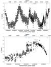 |
Fig. 1. AAVSO light curve of AG Car (top) and WRAY 15–751 (bottom) observed from January 1, 1982, to April 20, 2021. The solid blue lines represent the heliocentric Julian dates of the archival spectroscopy, and the dashed red line shows the heliocentric Julian date of the interferometric observation. |
Because of the sensitivity of the instruments, the interferometric sample consists of stars brighter than H = 5 mag in the northern and H = 6.5 mag in the southern hemisphere. These stars must also be brighter than 13.5 mag in the V band to be detected in the optical with 1−2 m class telescopes, which prevents us from observing in interferometry the objects that are very extincted. Because of these constraints, our interferometric sample contains 15 stars for which we obtained data (ESO Program ID: 0102.D-0460, PI: Mahy). To extend this sample, we also used the interferometric results published for η Car by GRAVITY Collaboration (2018), HR Car by Boffin et al. (2016), and the Pistol star by Martayan et al. (2012). The total of interferometric targets is 18 stars.
As mentioned above, both the spectroscopic and interferometric samples analysed in our study contain 18 stars. Because the requirements for the observations are different, only 11 targets belong to both samples. The list of the spectroscopic targets is given in Table 1 and that of the interferometric targets is given in Table 2. We have marked objects that belong to both tables with an asterisk.
Sample of LBV-like stars with spectroscopic detection parameters.
Sample of LBV-like stars with interferometric detection parameters.
2.2. Spectroscopy
For stars with declinations higher than −25°, we collected observations with the High-Efficiency and high-Resolution Mercator Echelle Spectrograph (HERMES), which is mounted on the 1.2 m Mercator telescope (Raskin et al. 2011) at the Observatorio del Roque de los Muchachos in La Palma (Spain). The data were taken in high-resolution fibre mode, which has a resolving power of R = 85 000, and covers the 4000 − 9000 Å wavelength domain. The raw exposures were reduced using the dedicated HERMES pipeline, and we worked with the extracted cosmic-removed, merged spectra afterwards.
Between 2013 and 2020, we also obtained about 25 intermediate-resolution spectra of HD 168625, HD 168607 and P Cygni, among other luminous stars, with the robotic 1.2 m Telescopio Internacional de Guanajuato Robótico Espectroscópico (TIGRE; Schmitt et al. 2014) installed at the La Luz Observatory (Mexico). The TIGRE is equipped with the refurbished fibre-fed HEROS échelle spectrograph, which delivers spectra covering the wavelength ranges 3500−5600 Å (blue channel) and 5800−8800 Å (red channel) with a resolving power of about 20 000. Data reduction was made with the dedicated TIGRE/HEROS reduction pipeline (Mittag et al. 2010).
For stars in the southern hemisphere, we collected spectra with the High Resolution Spectrograph (HRS) on SALT (Bramall et al. 2010, 2012; Crause et al. 2014) under programme 2019-1-SCI-001 (PI: Miszalski). The data were taken in high-resolution mode for the brightest stars and in low-resolution mode for the faintest stars, with the cut-off around V = 10 mag. The data were reduced with the MIDAS pipeline (Kniazev et al. 2016) based on the échelle (Ballester 1992) and feros (Stahl et al. 1999) packages. We applied heliocentric corrections to the data and confirmed the wavelength calibrations by using the diffuse interstellar bands (DIBs) that are present within the wavelength coverage.
Finally, we retrieved spectra from the European Southern Observatory (ESO) archives observed with FEROS, UVES, HARPS, and X-shooter. The Fibre-fed Extended Range Optical Spectrograph (FEROS, Kaufer et al. 1999) is mounted on the MPG/ESO 2.2 m telescope at La Silla (Chile). FEROS provides a resolving power of R = 48 000 and covers the entire optical range from 3800 to 9200 Å. The data were reduced following the procedure described in Mahy et al. (2010, 2017).
Some stars were observed with the UV and Visible Echelle Spectrograph (UVES, Dekker et al. 2000) mounted on the 8.2 m Unit Telescope 2 (UT2) of the ESO Very Large Telescope (VLT) at the Paranal observatory (Chile). UVES has a resolving power of R = 80 000 and, depending on the setup, covers different wavelength ranges from the near-UV to optical domains. The spectra were reduced with the UVES pipeline data reduction software.
High-resolution, optical spectra were acquired with the High Accuracy Radial velocity Planet Searcher (HARPS, Mayor et al. 2003) spectrograph attached to the 3.6 m telescope at La Silla Observatory (Chile). In the high-efficiency (EGGS) mode, the spectral range covered is 3780−6910 Å and the resolving power R ∼ 80 000. The data were reduced with the HARPS pipeline.
For very extincted objects, we also found archival spectra collected with X-shooter (Vernet et al. 2011) on the ESO/VLT UT2. X-shooter is an intermediate-resolution (R ∼ 4000 − 17 000) slit spectrograph covering a wavelength range from 3000 to 25 000 Å, divided over three arms: UV-Blue (UVB), visible (VIS), and near-infrared (NIR). Because the objects are very extincted, only the NIR arm was used to measure the radial velocities (RVs).
Unlike O-type stars on the main sequence, LBV-like spectra may display spectral lines with P Cygni profiles or in emission. When they are in emission, these lines are smaller than emission lines visible in WR spectra, however, which facilitates the definition of the continuum in LBV-like spectra. To define this continuum, we focused on wavelength regions free from P Cygni profiles or emission lines. We reconstructed the continuum using splines of low order over limited wavelength windows. The observed spectra were then divided by the continuum to yield the normalised spectra.
2.3. Interferometry
The bulk of the interferometric observations has been obtained at ESO (PI: Mahy, Program ID: 0102.D-0460) with the Very Large Telescope Interferometer (VLTI). All long-baseline interferometric data were obtained with the Precision Integrated-Optics Near-infrared Imaging ExpeRiment (PIONIER) combiner (Le Bouquin et al. 2011, 2012) and the four auxiliary telescopes of the VLTI. We used the “large” (A0-G1-J2-J3) and “small” (A0-B2-C1-D0) configurations with the auxiliary telescopes. PIONIER is a four-beam interferometric combiner in the near-infrared H-band (central wavelength of 1.65 μm). The H-band is covered by six wavelength channels (R ∼ 40). This instrument provides two observables: the squared visibilities (V2) that are related to the size of the target, and closure phases (CP) that are related to the degree of (non-)point-symmetry. Data were reduced and calibrated with the pndrs package described in Le Bouquin et al. (2011). The statistical uncertainties typically range from 0.3° to 12° degrees for the CP and from 1 to 6% for the V2, depending on target brightness and atmospheric conditions.
Each observation sequence of the targets in our sample was bracketed by two observations of calibration stars in order to master the instrumental and atmospheric response. These calibrators were found using SearchCal2 and selected to be close to the science object both in terms of position (within ∼2°) and magnitude (within ±1.5 mag).
We also used the Michigan InfraRed Combiner-eXeter (MIRC-X, Anugu et al. 2020), which is a highly sensitive six-telescope interferometric imager installed at the CHARA Array (USA, ten Brummelaar et al. 2016). This instrument provides the V2 and CP observables as well. As this instrument combines the six telescopes of the CHARA array, a single observation with the six telescopes provides a sufficient (u, v)-coverage to detect and characterise a multiple system. MIRC-X is working in the H band as well. The observations used in this paper were obtained using the PRISM50 mode (R ∼ 50). MIRC-X data were reduced using the public pipeline3 described in Anugu et al. (2020).
3. Spectroscopic binary fraction
3.1. Radial velocities and the multiplicity criteria
In order to assess the RV variability of each star in a systematic way, we measured the Doppler shifts of a set of spectral lines in all available epochs (when the spectra were not affected by S-Dor cycles). The list of the selected spectral lines is given in Table 3. In addition, we took special care to only select spectra that were collected during the same hot quiescent or cool eruptive phase, given the spectral variability produced through the S-Dor cycles. These cycles have typical timescales of about a decade, which allowed us to probe long-period (longer than a few years) spectroscopic binary systems. The individual properties of the different campaigns are given in Table 1.
Spectral lines used for cross-correlation.
3.1.1. RV measurements
Before measuring the RVs, we carefully inspected the line profiles to look for clear signatures of putative companions that could move in anti-phase and that can be directly related to binarity. We did not find any spectral features that can be obviously related to a spectroscopic companion. We measured the RVs of the LBV-like stars by cross-correlating specific spectral lines or a whole region of lines with a template and then fit a parabola to the maximum region of the cross-correlation function (CCF, see Shenar et al. 2017). Figure 2 displays the CCF for three stars in our sample with the parabola fit of the maximum region. The choice of the lines or regions with which we cross-correlated depended on the target and on the wavelength coverage. Because the spectroscopic data have been collected with different instruments, their wavelength coverage is not the same in the whole dataset. We thus focused on spectral lines that are common to all the spectra (Table 3). We mainly favoured the selection of absorption lines because they are formed closer to the photosphere of the stars. Several objects only exhibit P-Cygni profiles or emission lines, however, as is the case for WR31a, or P Cyg for instance.
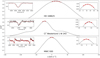 |
Fig. 2. Examples of CCF for three stars in our sample: HD 168625 (top), Cl* Westerlund 1 W 243 (middle), and MWC 930 (bottom). A zoom-in is displayed on the left side of the figure to show the comparison between the template (red) and one of the observations (black). The right side insets show a zoom-in on the top part of the CCF and in red the parabola fit with which we derived the RVs. |
The cross-correlation technique we used is based on Zucker (2003). Because modelling LBV-like spectra with an atmosphere-modelling code is complex (beyond the scope of this paper), the templates we used for the cross-correlation were initially chosen to be a template of the observations, that is, the spectrum with the highest signal-to-noise ratio (S/N). One of the advantages of using an observation as a template is that it is not affected by the fact that different spectral lines of LBV-like stars may imply different RVs due to their varying formation regions and asymmetric profiles. The spectra were then co-added in the rest frame of the star using these RVs to create a higher S/N template, which was then used to iterate on the RV measurements. We generally performed three iterations before obtaining the final sets of RVs. As in Shenar et al. (2017), the absolute RVs were obtained by cross-correlating the high S/N template with a suitable atmosphere model. Table A.1 gives the RV measurements for each spectral line or region and the mean values computed through all the lines or regions used for a given star. We also indicate the spectrum that was initially used as template for the cross-correlation. A full version of this table is available from the CDS.
3.1.2. Multiplicity criteria
To classify the LBV-like stars that can be assessed as binary candidates, we determined whether the measured RV variability was statistically significant. We considered the two statistical multiplicity criteria described in Sana et al. (2013). A star is classified as a likely spectroscopic binary if at least one pair of RVs measured at different epochs simultaneously satisfies these criteria:
-
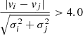 ,
, -
ΔRV = |vi − vj|> ΔRVmin,
where vi and vj are the individual RV measurements and σi and σj the respective 1σ errors on the RV measurements at epochs i and j. The first criterion defines a statistical test under which the null hypothesis of constant RV is rejected if, for a given star, any two RV measurements deviate significantly from one another. This criterion searches for significant variability at a 4σ level (Sana et al. 2013), considering the uncertainties on the measurements. The second criterion considers that the observed variability detected through the RV measurements is actually caused by orbital motion in a binary system and not through intrinsic variability that can be induced by pulsations, atmospheric activity, or, in the case of LBV-like stars, by wind effects. We therefore decided that two individual RV measurements had to deviate from one another by more than a minimum amplitude threshold ΔRVmin.
Previous studies of massive OB-type stars have used a variability threshold of 20 km s−1 (Sana et al. 2012, 2013; Bodensteiner et al. 2021; Banyard et al. 2021) to probe the multiplicity property in different metallicity environments (in the Galaxy, the Large and Small Magellanic Clouds). The stars in these different samples are massive stars on the main sequence, however, with little or undetectable line profile variability that could affect their multiplicity status. To distinguish between intrinsic variability and orbital motion among B-type stars in the LMC, Dunstall et al. (2015) adopted the threshold value of 16 km s−1 from their B-supergiant sample and used it for the entire population of B-type stars in the 30 Dor region. Simon-Diaz et al. (in prep.) investigated the effect of pulsations on the multiplicity properties in a large population of Galactic OB supergiants. They collected spectra of 56 Galactic OB supergiants, 13 O dwarfs and subgiants, and five early-B giants. They showed that the peak-to-peak amplitudes of RV measurements could reach up to 20−25 km s−1 for late-O and early-B supergiants and decrease to between 2 and 15 km s−1 for the O dwarfs and the late-B supergiants. For more evolved stars such as the Wolf-Rayet (WR) stars, Dsilva et al. (2020) observed two distinct kinks in their observed binary fraction computed for a sample of 12 objects classified as carbon-rich WR (WC) stars. The first kink was detected in the ranges between 5 and 10 km s−1 and the second between 12 and 19 km s−1, leading to an observed spectroscopic binary fraction of 0.58 and 0.33, respectively. These observed spectroscopic binary fractions, corrected for the observational biases, lead to an intrinsic binary fraction higher than 0.72.
Adopting different values as threshold obviously leads to different observed binary fractions. However, after correcting for observational biases, the choice of this threshold is taken into account, so that it does not affect the final binary fraction as long as a significant contamination by false positives is avoided. We investigated the effect of the choice of this threshold ΔRVmin on the observed spectroscopic binary fraction in the population of LBV-like stars. We varied this threshold between 0 and 100 km s−1 and calculated the observed spectroscopic binary fraction and the corresponding binomial error for each value of this threshold (Fig. 3). We performed a linear regression on the 0−35 km s−1 range and another linear regression on the 40−100 km s−1 range of the distribution. The kink shown by the different slopes in these two regressions is at ΔRVmin = 35 ± 3 km s−1. We used this value as a threshold, which provides us with an observed spectroscopic binary fraction of 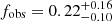 , where binomial statistics has been used to compute the uncertainty.
 |
Fig. 3. Observed binary fraction as a function of the adopted RV-variability threshold C. The vertical dotted line gives the adopted threshold value ΔRVmin = 35 ± 3 km s−1, which is indicated by the red line. The shaded area represents the ±1σ error. |
Our threshold is higher than those used for OB stars on the main sequence, for B supergiant populations, or for carbon-rich WR stars. As mentioned above, this choice was made to consider the intrinsic variability of these objects, but has the consequence that possible binary systems may not have been detected. Our sample consists of confirmed and dormant LBVs, therefore the choice of this threshold appears to be a good compromise, however, to discriminate against processes that lead to RV variability and that are not linked to binarity (e.g. pulsations, winds, and S-Dor cycles for the confirmed LBVs). We detect four binary candidates in the 18 objects of our sample. The detected candidates include HR Car, which has been detected in interferometry with an orbital period of about 2330 days (Boffin et al. 2016, and in prep.). MWC 314 and HD 326823 were detected by Lobel et al. (2013) and Richardson et al. (2011) through spectroscopy, as binary systems with orbital periods of about 6 and 61 days, respectively. Another system is identified as candidate binary: WRAY 15–751. Two other objects lie just below the threshold of 35 km s−1: MWC 930 and Cl* Westerlund 1 W 243. Both objects are confirmed LBVs. MWC 930 shows spectral variability, and its spectral lines are broad and show splitting (Miroshnichenko et al. 2005, 2014). Lobel et al. (2017) attributed this line splitting to optically thick central line emission produced in the inner ionised wind region. These authors suggested that this split is quite similar to the split observed in metal line cores of pulsating yellow hypergiants such as ρ Cas. Cl* Westerlund 1 W 243 was analysed by Ritchie et al. (2009), who claimed that this object might be a binary system with an undetected hot OB companion. However, the RV measurements were obviously not consistent with binarity, except if the system were seen under a low inclination, has a long period, or were highly eccentric. The threshold that we adopted does not select Schulte 12 as potential binary system. A period of 108 days has been reported from spectroscopy and X-rays by Nazé et al. (2019). This indicates that this period might be associated with another phenomenon than binarity, as suggested by these authors. We also fail to detect RV variability linked to binarity for HD 168625 or the Pistol star, while those two objects were possible wide-orbit binary systems (Martayan et al. 2016). Additionally, the observed spectroscopic binary fraction rises up to 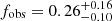 when we include the spectroscopic binary η Car in the sample (Damineli 1996).
The time coverage of our data varies from one object to the next because our spectroscopic data set is quite heterogeneous, but they allow us to probe timescales between 373 days for Cl* Westerlund 1 W 243 and about 7000 days for HD 168607 and HD 168625. In addition to confirming the orbital periods found for MWC 314 (Porb ∼ 60 days) and HD 326823 (Porb ∼ 6 days), no clear periodic signal has been found from our RV measurements. This suggests that either most of the LBV-like objects that pass our binary criteria are long-period systems or that the threshold is not strict enough. In any case, binary systems with orbital periods shorter than half the time coverage of the stars (see Table 1) would have been detected in our spectra, except if they were systems seen under a low inclination, with a low mass ratio, or with a high eccentricity. More details about the detection probability are given in Sect. 3.2.
3.2. Correction for observational biases
In order to assess the intrinsic multiplicity properties of the LBV-like objects, the observed binary fraction needs to be corrected for the observational biases. From our simulations and following the approach described in Sana et al. (2013), the probability of detecting our objects as binaries (Fig. 4) gives us an estimate of the sensitivity of our observations and provides us with a correction factor. The latter is multiplied by the observed spectroscopic binary fraction to estimate the intrinsic binary fraction.
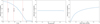 |
Fig. 4. Mean binary detection probabilities as a function of the orbital period (left), eccentricity (middle), and mass ratio (right). Known orbital periods of LBV-like stars in our sample are indicated by vertical lines. |
The first observational bias that we need to deal with is that the more spectra we obtain, the better we can assert the binarity detection through spectroscopy. To quantitatively assess the sensitivity of our data to the parameter space as well as to the properties of the undetected binary systems, we computed the binary detection probabilities.
We investigated the orbital configurations (period, eccentricity, and mass ratio) by assuming a mass range for the LBV-like objects that would yield RV signals that are compatible with our observational constraints. We ran one million Monte Carlo simulations tuned for each target of our sample. The period distribution was taken to be uniform over the logarithmic space and ranges from 1 to 105 days, the eccentricity between 0 and 0.95. All orbits with eccentricities lower than 0.03 were considered circular. The mass-ratio distribution was considered uniform and ranged from 0.01 to 1.0. Finally, the initial masses were taken for each star from Smith et al. (2019) from their position in the Hertzsprung-Russell diagram. We adopted a Salpeter initial mass function (IMF, with α = −2.35) for the primary masses; the tolerance varied from 5 to 40 M⊙. We emphasise, however, that the derived fractions are not sensitive to the slope of the IMF because the considered mass range is fairly limited. Our simulations assume that the orbits are randomly oriented in three-dimensional space, that the time of periastron passage is uncorrelated with respect to the start of the RV campaign, and that the orbital parameters are uncorrelated. To detect one system as a binary, it needs to fulfill the same criteria as we adopted for our analysis (Sect. 3.1.2).
Figure 4 shows the average detection probability curves of our spectroscopic campaign computed from all the objects in our sample. Globally, the orbital periods shorter than 102 days are well covered, and a detection probability close to 75% is reached. If the binary systems have orbital periods within the range 102 − 103 days, the detection probability drops to between 42 and 73%. For extremely long-period systems (between 103 and 104 days), the detection probabilities fall from 42% to 3%, showing the difficulty of constraining them from spectroscopy and the need for other observational techniques such as interferometry or high-contrast imaging.
Our campaign is sensitive to orbital periods up to 103 days, therefore the overall detection probability over that period is about 42%. Adopting different parameter distributions would provide different values, however. As mentioned by Bodensteiner et al. (2021), this affects the intrinsic binary fraction within an error of about 5%. While the overall observed spectroscopic binary fraction is estimated to be  (including η Car, see Sect. 3.1.2), the intrinsic bias-corrected binary fraction is therefore computed to be
  for the Galactic LBV-like population.
4. Interferometric companion detection
4.1. Multiplicity fraction and number of companions
To search for astrometric companions among LBV-like stars, we used the CANDID code4 (Gallenne et al. 2015). CANDID is a set of PYTHON tools that was specifically created to systematically search for high-contrast companions. CANDID provides the best fit from a Levenberg-Marquardt minimisation that performs a systematic exploration of the parameter space. The best fit is found assuming a disc for the primary, an unresolved secondary, and some background flux. A disc used to mimic the primary can correspond to stellar photosphere or to any material around the stars that are too close to the stellar surface to be resolved by interferometry (wind, dust torus, etc.). The reliability of the fit is only based on whether the grid used to search for a companion is fine enough (Gallenne et al. 2015). All the detections performed by CANDID are given in Table 2.
We detect 11 companions out of 15 LBV-like objects in our sample with a high number of sigmas (> 7σ). For two of these companions, the best-fit models provided by CANDID fail to provide all the parameters, even though their fits are reliable (HD 168625 and Schulte 12). For HD 168625, the CANDID best-fit model did not allow us to fit the primary diameter, which tends to indicate that the primary star is unresolved. For Schulte 12, the separation and position angle could not be derived. The best fit provided by CANDID is reliable, but the detected companion has a separation larger than 100 mas from the central star, that is, it is outside the interferometric field of view of MIRC-X with the current resolution.
To these 11 companions, we have to add 3 objects for which companions were already detected: η Car (observed with VLTI/GRAVITY, GRAVITY Collaboration 2018), HR Car (Boffin et al. 2016), and the Pistol star (Martayan et al. 2012). When these stars are added, the astrometric binary fraction rises from fastro = 0.61 to fastro = 0.78 (14 objects out of 18). Of the 14 companions, 7 have an angular separation (ρ) between 1 and 10 mas, 5 have 10 < ρ < 100 mas, and one has ρ > 100 mas (Table 2). Finally, the companion of Schulte 12 must have an angular separation between 65 mas (Caballero-Nieves et al. 2014; Maryeva et al. 2016) and about 100 mas. Because of the interferometric field of view and bandwidth-smearing, PIONIER (MIRC-X, PRISM50 mode) together with the VLTI (CHARA) baselines are hardly sensitive to any binaries with ρ > 150 mas (ρ > 100 mas).
For the targets that overlap in the spectroscopic and interferometric samples, it is unclear whether the detected companions are the same. Only dedicated monitoring will help us to understand the real configurations of these systems. No pair with similar or relatively close brightness (Δmag < 2, Fig. 5) has been detected in our sample. All the detected companions are much fainter than the companions found around O-type stars (Sana et al. 2014). In addition, over half of the detected companions have a Δmag > 4 in the H band, that is, lie beyond the detection limit of the O-star survey. Despite our improved sensitivity, we are only able to detect a maximum of one companion around LBV-like objects, while for the O-type star population, the average number of companions detected by interferometry is fc = 2.1 ± 0.2 (Sana et al. 2014).
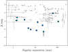 |
Fig. 5. Magnitude difference (Δ mag) vs. angular separations (ρ) for the detected companions. Grey dots correspond to the detected pairs by PIONIER and SAM in the O-type star population (Sana et al. 2014). |
The relative flux fractions of the secondaries are converted into flux ratios. From the luminosities of the LBVs (Smith et al. 2019; Bailer-Jones et al. 2021, see also Table 4), these flux ratios provide us with information about the nature of the companions. The luminosities that we can derive for the companions range between 2.8 < log(L/L⊙) < 5.4, but they obviously also depend on whether we consider the distances given by Smith et al. (2019) or by Bailer-Jones et al. (2021). Even though we do not know the effective temperatures of the companions, these luminosities suggest that companions are OB stars on the main sequence. We cannot reject the hypothesis that these companions might be RSG, although this is less likely given evolutionary considerations. The fact that we do not observe companions with luminosities higher than log(L/L⊙)∼5.4 highlights that these companions cannot be classical WR stars formed through a single-star channel, nor can they be early O-type or WNLh stars, that is, WR stars on the main sequence (see Sect. 5.3).
Surrounding environment and physical parameters of the primary.
As mentioned above, CANDID was developed to detect faint companions by assuming a disc for the primary, an unresolved secondary, and additional background flux. However, this tool does not allow different models. Because LBVs are characterised by strong winds, other types of models that are able to mimic the objects and their winds also need to be tested. For this purpose, we complement our study by using Lyons Interferometric Tool prototype (LITPRO5, Tallon-Bosc et al. 2008). We assumed a type of model composed of a disc or point-like source (both were tested) to model the LBV-like objects, and a Gaussian profile modelling the winds and centred on the star. We stress that using a point-like source rather than a disc provides us with similar chi-square values. The aim of LITPRO is to find the parameters that result in the highest probability that the data are given by a certain theoretical model. For eight stars in our sample (HD 160529, P Cyg, HD 168607, HD 168625, ζ Sco, Schulte 12, Cl* Westerlund 1 W 243, and HD 326823), the fits performed by CANDID provide a lower chi-square, suggesting that these objects are binary systems. For three stars (AG Car, [GKF2010] MN46, and [GKF2010] MN48), the measured chi-squares with CANDID and LITPRO are equivalent and the difference between the two models become insignificant. Our analysis shows that the binary fraction among LBV-like objects is between 53 and 73%. If we also consider HR Car, the Pistol star, and η Car, which are already reported as binaries, the binary fraction rises to between 61 and 78%. Therefore the binary fraction is fastro = 0.70 ± 0.09. We stress, however, that more observations are needed to confirm the binary status of our objects and derive their orbital motions. In Sect. 5 we discuss the implications assuming that the faint companions that have been detected with CANDID are physically bound to the LBV-like objects.
5. Discussion
5.1. Physical parameters of the LBV-like objects
Using interferometry to characterise the multiplicity of LBV-like objects allows us to derive the primary diameters, and by knowing the distances of the stars, to measure their radii directly. Based on our analysis, we have detected companions for 11 objects in our sample. We list these objects in Table 4. We also include HR Car as this star was intensively monitored by Boffin et al. (2016) and because the primary diameters have been published. We retrieve from Smith et al. (2019, and references therein) the luminosities and the effective temperatures of the LBV-like objects from their locations in the HRD. From the luminosities and effective temperatures, we derived their radii (reported as Revol, from  ). The radii measured from interferometry are scaled relative to the distances of the stars (reported as Rinterfero in Table 4). Table 4 summarises the measured radii, luminosities, effective temperatures, and distances of the stars reported by Smith et al. (2019) and Bailer-Jones et al. (2021). We also indicate the size and shape of their circumstellar nebulae, when they have been detected. Certain distances provided by Smith et al. (2019) differ from the distances given by the Gaia early-Data Release 3 (eDR3, Bailer-Jones et al. 2021), such as those for Cl* Westerlund 1 W 243 and [GKF2010] MN46. A comparison is displayed in Fig. 6. We stress, however, that independent studies have shown that for Cl* Westerlund 1 W 243, its real distance is more between 2.6 and 4.1 kpc (Aghakhanloo et al. 2020; Beasor et al. 2021). However, considering different distances does affect the measurements of the stellar radii, but would not change the conclusions of our study.
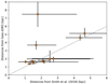 |
Fig. 6. Comparison between distances from Smith et al. (2019) and from Gaia eDR3 (Bailer-Jones et al. 2021). |
In general, the agreement between the interferometric and evolutionary radii is excellent within the error bars, as is the case notably for Schulte 12, [GKF2010] MN48, Cl* Westerlund 1 W 243, and HR Car. For three confirmed LBVs, P Cyg, HD 168607, and AG Car, the radii derived from interferometry are slightly larger than those inferred from the effective temperatures and luminosities. One possible explanation is that LBVs can produce optically thick winds around their photosphere, which causes the stars to appear larger than they actually are. Another explanation is that they can present variations in their stellar parameters due to their strong variability or S-Dor cycles that would modify the properties of the stars between the time of our observations and the results listed in Smith et al. (2019). AG Car is well observed photometrically to probe its variability, which is linked to its S-Dor cycle. When our interferometric observation was collected, AG Car was close to its visual maximum phase, which is when the star appears to be cool and eruptive (marked with the red line in Fig. 1). This phase is characterised by a low effective temperature (∼9 kK) and a large radius. The radius we measure from interferometry supports the idea that AG Car went through this disruptive phase.
The strongest discrepancy between the radii measured from interferometry and the radii computed from the position in the HRD is observed for HD 326823 (see Table 4). HD 326823 was found to be a close binary system with an orbital period of 6.1 days (Richardson et al. 2011). The companion detected in spectroscopy cannot be the same as that detected from interferometry, meaning that the system consists of a hierarchical triple system. According to Richardson et al. (2011), the inner binary system in HD 326823 is surrounded by a circumbinary disc (detected in spectroscopy through double-peaked emission profiles visible, notably, in the Fe II and Ni II lines). Interferometry does not allow us to resolve the inner system, but it allows us to model it with its circumbinary material by assuming a disc with a radius of about 120 − 130 R⊙ at the distance of the object. Richardson et al. (2011) have estimated the inner radius of the circumbinary region to be equal to 2.83a (where a is the semi-major axis of the inner system, i.e., between 30 and 50 R⊙, depending on the inclination of the inner system and the mass of the close-by companion).
We should stress that some objects in our sample are surrounded by large nebulae of ejected material, with sizes of several parsecs squared at their distances (given in Table 4). Based on the size of these ejecta (much larger than what we measure), it is unlikely that they affect the measurements of the stellar radius in interferometry. These nebulae are also very bright in the infrared (with peaks close to 24 μm), but remain faint in the H band. Their contributions in our observations are therefore not significant.
Finally, if the radii measured when we consider the distances of the stars are those of the photosphere of the LBVs, this favours the presence of companions on wide orbits. We note, however, that we cannot completely rule out the fact that the primaries might be short-period systems surrounded by circumbinary discs, as it is the case for HD 326823, but our spectroscopic campaign would have detected 90% of them.
5.2. LBV versus O star populations
Our analysis of a representative sample of Galactic LBVs in the Milky Way both from spectroscopy and interferometry yields a global binary fraction of 67 ± 11%. This fraction agrees with that derived among massive Galactic O-type stars (Sana et al. 2012, 2014). As emphasised in Sect. 5.1, one difference lies in the number of short- versus long-period systems. About 60% of binary systems containing massive OB stars have periods shorter than 10 days, and 20% have orbital periods between 10 and 100 days (Sana et al. 2012; Almeida et al. 2017; Banyard et al. 2021; Villaseñor et al. 2021). The picture is significantly different for the population of Galactic LBV-like objects because only one (HD 326823) is clearly identified as a short-period system. The fact that there is a lack of short-period systems in the LBV-like star population is expected because the LBV-like objects have relatively large radii that prevent any close companions (Sect. 5.1).
Because the secondary components are on long-period orbits, we compared the companions around LBV-like stars with the companions detected through interferometry. We focused on the results provided by the Southern MAssive Star at High angular resolution (SMASH+, Sana et al. 2014) survey. This survey combined long-baseline interferometry with VLTI/PIONIER, aperture masking with VLT/NACO-SAM, and adaptive optics with VLT/NACO-FOV to search for companions with separations in the range of 1−8000 mas. We only compared the two populations up to a separation of 120 mas, which is the limit of detection in interferometry. As mentioned in Sect. 2.3, the luminosities of the companions orbiting LBV-like stars range between log(L/L⊙) = 2.8 and 5.4, meaning that they are classified between late-B and mid-O if they are on the main sequence, but they can also be more evolved and be classified as yellow or red supergiants if they left the main sequence. From SMASH+, the spectral types of the companions range between log(L/L⊙) = 3.4 and 5.7, that is, between mid-B and early-O. Because the most massive stars in these systems are on the main sequence, it is more likely that their companions are also located on the main sequence. When we assume that the companions around LBVs are still on the main sequence, they are therefore not significantly less massive than the companions around O-type stars.
The distribution of angular separations of the companions in the LBV-like star population were compared to those found around O-type stars (top panel of Fig. 7) by performing a Kuiper test on the two samples. This test indicates that the likelihood is only 4% that the two samples come from the same parent distribution (p-value = 0.04). About 80% of the LBV-like stars have a companion closer to 20 mas, while this value drops to approximately 60% in the O-star sample. When we only consider the hierarchical triple systems in the O-star sample, that is, objects composed of an inner short-period spectroscopic binary and an outer star orbiting it, the angular separation distribution also looks different, and we can also reject the null hypothesis that the two distributions are drawn from the same parent distribution (p-value = 0.03).
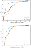 |
Fig. 7. Top: cumulative distribution of the companion separations in the LBV-like star population (in blue) and in the O-type star population detected through the SMASH+ survey (Sana et al. 2014). Bottom: same as in the top panel, but considering the distances of the stars from the eDR3 Gaia catalogue. |
When we take the distances of these systems into account (bottom panel of Fig. 7), the separation distributions still look different. We performed a Kuiper test to compare the separation distribution of the LBV-like stars and that of the whole sample of O-type stars. We reject the null hypothesis that the two samples come from the same parent distribution (p-value = 0.05). When we focus only on the hierarchical triple systems, the test also shows that the likelihood is 24% that the two distributions are compatible (p-value = 0.24). We emphasise that the comparison of the triple systems and the whole sample of O-type stars shows that the two distributions are also compatible (p-value = 0.99). About 80% of the LBV-like stars have a companion closer than 50 AU, however, while this number drops to 53% in the O-star population (against 47% when we only consider the triple systems). Regardless of whether LBV-like stars are formed through single- or binary-evolutionary channel, one explanation of this difference in the distributions could come from the fact that the systems hosting LBV-like stars are more evolved than those hosting O-type stars. However, only a good knowledge of the orbital parameter distributions (orbital period, eccentricity, and mass ratio) would give us insight into the role of the LBVs in the evolution of massive stars.
5.3. Binary evolution
The traditional view of massive star evolution is that massive O-type stars evolve to classical WR stars (hydrogen free) by stripping their outer layers through their powerful stellar winds. With the detection of inhomogeneities (or clumps) in their wind, these mass-loss rates were considerably revised downwards in the massive star population (Eversberg et al. 1998; Vink et al. 2001; Bouret et al. 2003; Björklund et al. 2021), and when integrated over the stellar lifetime of these stars, they are not sufficient to enable a direct evolution between the massive stars on the main sequence and the WR phase. The LBV evolutionary phase justifies the transition between these two evolutionary stages. It is thought to be extremely brief (104 − 105 yr) in comparison with the lifetime of a massive star (∼107 yr), and during this time span, their nebulae are expected to form through giant eruptions (Mahy et al. 2016).
When we consider single-star evolution to explain the existence of LBVs, LBVs must only form in long-period systems so that there is no interaction with their companion during their evolution. In these systems, the two components are expected to evolve like single stars most of their life. Sixty-eight objects were reported as confirmed or candidate LBVs in the catalogue of Nazé et al. (2012). Considering the lifetime of the LBV phase and the number of O-type stars in the Milky Way (Maíz Apellániz et al. 2011), about 1% of the O stars will enter into a phase of LBV. This is less than the number of O-type stars that are expected to evolve like single stars either isolated or as members of binary systems with wide orbits (Sana et al. 2012; de Mink et al. 2014). Therefore we cannot exclude that LBVs do indeed form through a single-star channel.
While 30% of the O-stars on the main-sequence are expected to evolve like single stars, most of the stars born as O-type stars will interact during their lifetime. To determine whether the abundance of short-period systems in the O-star population (∼60%) might be reconcilable with the fact that the majority of LBV-like stars are on wide-orbit systems, we focus on the same approach as was presented in Bodensteiner et al. (2020). In this approach, the current orbital properties of LBVs (Porb > 1000 days, and mass ratio q = (MLBV/Mcomp) < 20) can be used to assess the initial conditions of the progenitor systems. Assuming circular orbits, a constant mass transfer efficiency, and ignoring other mechanisms for angular momentum loss from the system, the orbital period can be computed analytically as a function of the mass ratio (we refer to Soberman et al. 1997; Bodensteiner et al. 2020, for the equations). Figure 8 shows the result of evaluating the initial orbital periods and mass ratios for different values of the currently observed mass ratio within our range of uncertainty. We considered two different cases: when the mass transfer is (1) conservative and (2) fully non-conservative. In the case of conservative mass transfer and assuming an initial mass ratio of q = 1/3, it is unlikely that close binary systems (with initial orbital periods shorter than 10 days) can evolve to form binary systems with periods of about one thousand days. When we consider a fully non-conservative mass transfer, however, these initially tight systems can evolve to form long-period systems (Porb ≳ 103 days), but require a current mass ratio higher than 10. Therefore we cannot rule out that detached short-period systems on the main-sequence will evolve to form long-period systems. In this mass-transfer scenario, the initial primary star would undergo a case A (if still on the main sequence) or an early case B (post-main sequence) mass transfer. This initial primary star, or mass donor, would lose mass and angular momentum and would be stripped of its hydrogen envelope, leading to the formation of a WN star. The initial secondary would accrete this material, inverting the mass ratio. This component, or mass gainer, would gain mass and angular momentum, resulting in a rapid rotator and rejuvenated star. While the mass donor would look like a WR star, the mass gainer could have all the characteristics of LBV stars (e.g. rapid rotation, chemical enrichment, see Groh et al. 2009b). Based on the luminosities that we derived for the companions of LBV-like stars (Sect. 2.3), we cannot exclude that some of these companions, but not all of them, might be stripped WR stars (Shenar et al. 2020). In this stage of our analysis, we are not yet able to characterise the nature of the companions any further, nor can we conclude whether they would have the stellar properties reminiscent of donor stars (Mahy et al. 2020).
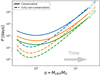 |
Fig. 8. Past orbital evolution of systems assuming present-day mass ratios of q = 10, 15, and 20. During mass transfer phases, time increases towards the right in this figure. Each curve has been computed assuming a current orbital period of 3000 days. The left-most point corresponds to an arbitrary choice of q = 1/3. |
Another scenario in which short-period systems would be transformed into wide-orbit binaries would involve merging either through a common-envelope phase in an initial binary system, leading to a single LBV star, or in a hierarchical system, leading to a binary system with a wide orbit. While we have shown that the separations between main-sequence O-type stars (in binary or triple systems) or LBV-like objects with their companion are not compatible, only the orbital parameter distributions derived for LBV-like stars would allow us to quantitatively test whether these objects might be formed from the binary channel. It is therefore of paramount importance to perform more intensive interferometric monitoring of these stars to derive their orbital parameters.
Mass transfer and merger have been evoked by Smith & Tombleson (2015), which was later supported by Aghakhanloo et al. (2017), to justify that most of the LBVs are found to be surprisingly isolated when compared to the O- and WR-star populations. While the results from these analyses were strongly debated, if LBVs are kicked mass gainers, they must appear as runaways (at least for some of them). While massive O-type runaways have been detected in short-period binary systems, none has been detected as having companions on wide orbits (Sana et al. 2014). It would be surprising if after being ejected from a binary or multiple system, so many LBVs would still be found in long-period binary systems. This clear dichotomy suggests that the kick scenario is unlikely.
Finally, some (confirmed and candidate) LBVs are surrounded by a circumstellar nebula. The origin of these nebulae is still unknown and might come at this stage from a giant eruption, a merger, and to a lesser extent, non-conservative mass transfer. A link might exist between multiplicity and the presence of a nebula. In Table 4 we list the morphology and the size of the nebulae detected around LBV-like stars. We display in Fig. 9 the cumulative distributions of the angular separations of companions around LBV-like stars with and without a circumstellar nebula. We cannot reject the null hypothesis that the two distributions are drawn from the same parent distributions (p-value = 0.78). This may also indicate that the kinematics of the outflows in these nebulae deserve to be better studied to verify whether inclination effects may misrepresent the nebulae as spherical rather than bipolar. At this stage, the question about the presence of nebulae around LBVs and possible mass-transfer episodes remains open. We did not detect any evidence either between physical or projected separations of the companions and the size of the nebulae. We also computed a Kuiper test between the populations of confirmed LBVs and candidate LBVs to detect any differences between these two populations and failed to find any (p-value = 0.85). This result must be taken with caution, however, given the small-number statistics.
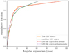 |
Fig. 9. Cumulative distribution of the companion separations in the LBV-like star population (true LBVs in orange, candidate LBVs in green, surrounded by a nebula in red, and without a nebula in magenta). |
6. Conclusions
We performed a dedicated search for binary companions in a Galactic LBV-like star population. We combined high-resolution, high-quality spectroscopic data with interferometric observations to probe separations in the range between 0.1 mas to 100 mas. Our spectroscopic and interferometric samples consist of 18 objects each, and 11 objects appear in both samples.
After correcting for the spectroscopic observational biases, we found a spectroscopic binary fraction of  % over the period range between 1 and 1000 days. From our interferometric data, we also find a high binary fraction of 70 ± 9%, that is, for projected separations up to 100−150 mas, depending on the instruments that were used. Ninety percent of the confirmed LBVs in our sample do have a companion, but this fraction decreases to about 45% for the candidate LBVs. Even though the observations do not allow us to probe the orbital parameter distributions, we measured the physical radii of LBV-like stars through interferometry. These radii suggest that our objects in binary systems must have companions on a wide orbit. This significantly differs from the O and early B-type stars that are mainly found in systems with orbital periods between 1 and 10 days. We showed that we can reproduce the currently observed parameters (Porb ≳ 103 days) with a tight progenitor system that has undergone a full non-conservative case A mass transfer. Another scenario can also explain the formation of wide-orbit systems: a merger in binary or hierarchical triple systems. This challenges the traditional view that O-type stars evolve to WR stars through a transitory LBV phase.
The interferometric data also allowed us to characterise the luminosities of the companions. We estimated that the companions have luminosities between log(L/L⊙) = 2.8 and 5.4, meaning that they are classified from late-B to mid-O if they are on the main sequence. These luminosities show that early-O or WNL star can be excluded as companions of LBV-like stars. We do not have any indications about the effective temperatures of the companions, therefore we cannot rule out that the companions might be RSGs. Additionally, even if it is unlikely, we cannot rule out either that they might be classical WR stars. However, the luminosity range that we derived for the companions means that if they are classified as WR stars, there are strong indications that they must have formed through binary interactions.
Our study for the first time places a strong constraint on the binary fraction in Galactic confirmed and candidate LBVs and on the exact radii of these stars. However, without a clear characterisation of the orbital properties, the physical associations with the central LBV-like objects only rely on statistical arguments. This emphasises the need for additional data to clearly confirm the binarity of those objects. These distributions are crucial to quantitatively test the evolution of massive stars.
Acknowledgments
We thank the anonymous referee for his/her very valuable comments that improve the quality of the paper. L.M. thanks the European Space Agency (ESA) and the Belgian Federal Science Policy Office (BELSPO) for their support in the framework of the PRODEX Programme. H.S. acknowledges support from the FWO_Odysseus program under project G0F8H6N. The research leading to these results has received funding from the European Research Council (ERC) under the European Union’s Horizon 2020 research and innovation programme (grant agreement numbers 772225: MULTIPLES). J.K. acknowledges support from the research council of the KU Leuven under grant number C14/17/082 and from FWO under the senior postdoctoral fellowship (1281121N). A.L. acknowledges funding received in part from the European Union Framework Programme for Research and Innovation Horizon 2020 (20142020) under the Marie Sklodowska-Curie grant Agreement No. 823734 (Physics of Extreme Massive Stars). R.M. acknowledges funding from the South African Claude Leon Foundation. We are also thankful to Tomer Shenar, Pablo Marchant, and Karan Dsilva for very interesting discussions. The Mercator telescope is operated by the Flemish Community on the island of La Palma at the Spain Observatory del Roche de los Muchachos of the Instituto de Astrofisica de Canarias. Mercator and Hermes are supported by the Funds for Scientific Research of Flanders (FWO), the Research Council of KU Leuven, the Fonds National de la Recherche Scientifique (FNRS), the Royal Observatory of Belgium, the Observatoire de Genève, and the Thüringer Landessternwarte Tautenburg. We thanks all the observers who collected the data with Hermes. The TIGRE facility is funded and operated by the universities of Hamburg, Guanajuato, and Liège. This paper is based in part on spectroscopic observations made with the Southern African Large Telescope (SALT) under programme 2019-1-SCI-001 (PI: Miszalski). We are grateful to our SALT colleagues for maintaining the telescope facilities and conducting the observations. This research has made use of the SIMBAD database, operated at CDS, Strasbourg, France and of NASA’s Astrophysics Data System Bibliographic Services. We are grateful to the staff of the ESO Paranal Observatory for their technical support.
References
- Aadland, E., Massey, P., Neugent, K. F., & Drout, M. R. 2018, AJ, 156, 294 [NASA ADS] [CrossRef] [Google Scholar]
- Aghakhanloo, M., Murphy, J. W., Smith, N., & Hložek, R. 2017, MNRAS, 472, 591 [NASA ADS] [CrossRef] [Google Scholar]
- Aghakhanloo, M., Murphy, J. W., Smith, N., et al. 2020, MNRAS, 492, 2497 [NASA ADS] [CrossRef] [Google Scholar]
- Almeida, L. A., Sana, H., Taylor, W., et al. 2017, A&A, 598, A84 [NASA ADS] [CrossRef] [EDP Sciences] [Google Scholar]
- Anugu, N., Le Bouquin, J.-B., Monnier, J. D., et al. 2020, AJ, 160, 158 [NASA ADS] [CrossRef] [Google Scholar]
- Bailer-Jones, C. A. L., Rybizki, J., Fouesneau, M., Demleitner, M., & Andrae, R. 2021, AJ, 161, 147 [Google Scholar]
- Ballester, P. 1992, Eur. South. Obs. Conf. Workshop Proc., 41, 177 [NASA ADS] [Google Scholar]
- Banyard, G., Sana, H., Mahy, L., et al. 2021, ArXiv e-prints [arXiv:2108.07814] [Google Scholar]
- Beasor, E. R., Davies, B., Smith, N., Gehrz, R. D., & Figer, D. F. 2021, ApJ, 912, 16 [NASA ADS] [CrossRef] [Google Scholar]
- Björklund, R., Sundqvist, J. O., Puls, J., & Najarro, F. 2021, A&A, 648, A36 [EDP Sciences] [Google Scholar]
- Bodensteiner, J., Shenar, T., Mahy, L., et al. 2020, A&A, 641, A43 [NASA ADS] [CrossRef] [EDP Sciences] [Google Scholar]
- Bodensteiner, J., Sana, H., Wang, C., et al. 2021, A&A, 652, A70 [NASA ADS] [CrossRef] [EDP Sciences] [Google Scholar]
- Boffin, H. M. J., Rivinius, T., Mérand, A., et al. 2016, A&A, 593, A90 [NASA ADS] [CrossRef] [EDP Sciences] [Google Scholar]
- Bouret, J. C., Lanz, T., Hillier, D. J., et al. 2003, ApJ, 595, 1182 [NASA ADS] [CrossRef] [Google Scholar]
- Bramall, D. G., Sharples, R., Tyas, L., et al. 2010, SPIE Conf. Ser., 7735, 77354F [NASA ADS] [Google Scholar]
- Bramall, D. G., Schmoll, J., Tyas, L. M. G., et al. 2012, SPIE Conf. Ser., 8446, 84460A [NASA ADS] [Google Scholar]
- Caballero-Nieves, S. M., Nelan, E. P., Gies, D. R., et al. 2014, AJ, 147, 40 [CrossRef] [Google Scholar]
- Clark, J. S., Larionov, V. M., & Arkharov, A. 2005, A&A, 435, 239 [NASA ADS] [CrossRef] [EDP Sciences] [Google Scholar]
- Crause, L. A., Sharples, R. M., Bramall, D. G., et al. 2014, SPIE Conf. Ser., 9147, 91476T [Google Scholar]
- Damineli, A. 1996, ApJ, 460, L49 [NASA ADS] [Google Scholar]
- Davidson, K., Humphreys, R. M., Weis, K., et al. 2016 ArXiv e-prints [arXiv:1608.02007] [Google Scholar]
- de Mink, S. E., Sana, H., Langer, N., Izzard, R. G., & Schneider, F. R. N. 2014, ApJ, 782, 7 [Google Scholar]
- Dekker, H., D’Odorico, S., Kaufer, A., Delabre, B., & Kotzlowski, H. 2000, in Optical and IR Telescope Instrumentation and Detectors, eds. M. Iye, & A. F. Moorwood, SPIE Conf. Ser., 4008, 534 [Google Scholar]
- Dsilva, K., Shenar, T., Sana, H., & Marchant, P. 2020, A&A, 641, A26 [NASA ADS] [CrossRef] [EDP Sciences] [Google Scholar]
- Dunstall, P. R., Dufton, P. L., Sana, H., et al. 2015, A&A, 580, A93 [NASA ADS] [CrossRef] [EDP Sciences] [Google Scholar]
- Eversberg, T., Lépine, S., & Moffat, A. F. J. 1998, ApJ, 494, 799 [NASA ADS] [CrossRef] [Google Scholar]
- Gal-Yam, A., Leonard, D. C., Fox, D. B., et al. 2007, ApJ, 656, 372 [NASA ADS] [CrossRef] [Google Scholar]
- Gallagher, J. S. 1989, in Close Binary Models for Luminous Blue Variable Stars, eds. K. Davidson, A. F. J. Moffat, & H. J. G. L. M. Lamers, 157, 185 [NASA ADS] [CrossRef] [Google Scholar]
- Gallenne, A., Mérand, A., Kervella, P., et al. 2015, A&A, 579, A68 [NASA ADS] [CrossRef] [EDP Sciences] [Google Scholar]
- Gräfener, G., Owocki, S. P., & Vink, J. S. 2012, A&A, 538, A40 [NASA ADS] [CrossRef] [EDP Sciences] [Google Scholar]
- Grassitelli, L., Langer, N., Mackey, J., et al. 2021, A&A, 647, A99 [NASA ADS] [CrossRef] [EDP Sciences] [Google Scholar]
- GRAVITY Collaboration (Sanchez-Bermudez, J., et al.) 2018, A&A, 618, A125 [NASA ADS] [CrossRef] [EDP Sciences] [Google Scholar]
- Groh, J. H., Hillier, D. J., Damineli, A., et al. 2009a, ApJ, 698, 1698 [NASA ADS] [CrossRef] [Google Scholar]
- Groh, J. H., Damineli, A., Hillier, D. J., et al. 2009b, ApJ, 705, L25 [NASA ADS] [CrossRef] [Google Scholar]
- Groh, J. H., Meynet, G., & Ekström, S. 2013, A&A, 550, L7 [NASA ADS] [CrossRef] [EDP Sciences] [Google Scholar]
- Humphreys, R. M., & Davidson, K. 1994, PASP, 106, 1025 [NASA ADS] [CrossRef] [Google Scholar]
- Humphreys, R. M., Weis, K., Davidson, K., & Gordon, M. S. 2016, ApJ, 825, 64 [NASA ADS] [CrossRef] [Google Scholar]
- Justham, S., Podsiadlowski, P., & Vink, J. S. 2014, ApJ, 796, 121 [NASA ADS] [CrossRef] [Google Scholar]
- Kaufer, A., Stahl, O., Tubbesing, S., et al. 1999, The Messenger, 95, 8 [Google Scholar]
- Kiewe, M., Gal-Yam, A., Arcavi, I., et al. 2012, ApJ, 744, 10 [NASA ADS] [CrossRef] [Google Scholar]
- Kniazev, A. Y., Gvaramadze, V. V., & Berdnikov, L. N. 2016, MNRAS, 459, 3068 [NASA ADS] [CrossRef] [Google Scholar]
- Koenigsberger, G., Georgiev, L., Hillier, D. J., et al. 2010, AJ, 139, 2600 [NASA ADS] [CrossRef] [Google Scholar]
- Lamers, H. J. G. L. M., & Nugis, T. 2002, A&A, 395, L1 [NASA ADS] [CrossRef] [EDP Sciences] [Google Scholar]
- Le Bouquin, J. B., Berger, J. P., Lazareff, B., et al. 2011, A&A, 535, A67 [NASA ADS] [CrossRef] [EDP Sciences] [Google Scholar]
- Le Bouquin, J. B., Berger, J. P., Zins, G., et al. 2012, SPIE Conf. Ser., 8445, 84450I [NASA ADS] [Google Scholar]
- Lobel, A., Groh, J. H., Martayan, C., et al. 2013, A&A, 559, A16 [NASA ADS] [CrossRef] [EDP Sciences] [Google Scholar]
- Lobel, A., Martayan, C., Mehner, A., & Groh, J. H. 2017, in The B[e] Phenomenon: Forty Years of Studies, eds. A. Miroshnichenko, S. Zharikov, D. Korčáková, & M. Wolf, ASP Conf. Ser., 508, 245 [NASA ADS] [Google Scholar]
- Maeder, A., & Meynet, G. 2000, A&A, 361, 159 [NASA ADS] [Google Scholar]
- Mahy, L., Rauw, G., Martins, F., et al. 2010, ApJ, 708, 1537 [NASA ADS] [CrossRef] [Google Scholar]
- Mahy, L., Hutsemékers, D., Royer, P., & Waelkens, C. 2016, A&A, 594, A94 [NASA ADS] [CrossRef] [EDP Sciences] [Google Scholar]
- Mahy, L., Damerdji, Y., Gosset, E., et al. 2017, A&A, 607, A96 [NASA ADS] [CrossRef] [EDP Sciences] [Google Scholar]
- Mahy, L., Sana, H., Abdul-Masih, M., et al. 2020, A&A, 634, A118 [NASA ADS] [CrossRef] [EDP Sciences] [Google Scholar]
- Maíz Apellániz, J., Sota, A., Walborn, N. R., et al. 2011, in Highlights of Spanish Astrophysics VI, eds. M. R. Zapatero Osorio, J. Gorgas, J. Maíz Apellániz, J. R. Pardo, & A. Gil de Paz, 467 [Google Scholar]
- Martayan, C., Blomme, R., Le Bouquin, J. B., et al. 2011, Bull. Soc. R. Sci. Liege, 80, 400 [NASA ADS] [Google Scholar]
- Martayan, C., Lobel, A., Baade, D., et al. 2012, in Circumstellar Dynamics at High Resolution, eds. A. C. Carciofi, & T. Rivinius, ASP Conf. Ser., 464, 293 [NASA ADS] [Google Scholar]
- Martayan, C., Lobel, A., Baade, D., et al. 2016, A&A, 587, A115 [NASA ADS] [CrossRef] [EDP Sciences] [Google Scholar]
- Maryeva, O. V., Chentsov, E. L., Goranskij, V. P., et al. 2016, MNRAS, 458, 491 [NASA ADS] [CrossRef] [Google Scholar]
- Mayor, M., Pepe, F., Queloz, D., et al. 2003, The Messenger, 114, 20 [NASA ADS] [Google Scholar]
- Miroshnichenko, A. S., Bjorkman, K. S., Grosso, M., et al. 2005, MNRAS, 364, 335 [NASA ADS] [CrossRef] [Google Scholar]
- Miroshnichenko, A. S., Manset, N., Zharikov, S. V., et al. 2014, Adv. Astron., 2014, E7 [CrossRef] [Google Scholar]
- Mittag, M., Hempelmann, A., González-Pérez, J. N., & Schmitt, J. H. M. M. 2010, Adv. Astron., 2010, 101502 [CrossRef] [Google Scholar]
- Moe, M., & Di Stefano, R. 2017, ApJS, 230, 15 [Google Scholar]
- Nazé, Y., Rauw, G., & Hutsemékers, D. 2012, A&A, 538, A47 [NASA ADS] [CrossRef] [EDP Sciences] [Google Scholar]
- Nazé, Y., Rauw, G., Czesla, S., Mahy, L., & Campos, F. 2019, A&A, 627, A99 [NASA ADS] [CrossRef] [EDP Sciences] [Google Scholar]
- Oudmaijer, R. D., & Parr, A. M. 2010, MNRAS, 405, 2439 [NASA ADS] [Google Scholar]
- Portegies Zwart, S. F., & van den Heuvel, E. P. J. 2016, MNRAS, 456, 3401 [NASA ADS] [CrossRef] [Google Scholar]
- Raskin, G., van Winckel, H., Hensberge, H., et al. 2011, A&A, 526, A69 [CrossRef] [EDP Sciences] [Google Scholar]
- Richardson, N. D., Gies, D. R., & Williams, S. J. 2011, AJ, 142, 201 [Google Scholar]
- Ritchie, B. W., Clark, J. S., Negueruela, I., & Najarro, F. 2009, A&A, 507, 1597 [NASA ADS] [CrossRef] [EDP Sciences] [Google Scholar]
- Sana, H., de Mink, S. E., de Koter, A., et al. 2012, Science, 337, 444 [Google Scholar]
- Sana, H., de Koter, A., de Mink, S. E., et al. 2013, A&A, 550, A107 [NASA ADS] [CrossRef] [EDP Sciences] [Google Scholar]
- Sana, H., Le Bouquin, J. B., Lacour, S., et al. 2014, ApJS, 215, 15 [Google Scholar]
- Sanyal, D., Grassitelli, L., Langer, N., & Bestenlehner, J. M. 2015, A&A, 580, A20 [NASA ADS] [CrossRef] [EDP Sciences] [Google Scholar]
- Schmitt, J. H. M. M., Schröder, K. P., Rauw, G., et al. 2014, Astron. Nachr., 335, 787 [NASA ADS] [CrossRef] [Google Scholar]
- Shenar, T., Richardson, N. D., Sablowski, D. P., et al. 2017, A&A, 598, A85 [NASA ADS] [CrossRef] [EDP Sciences] [Google Scholar]
- Shenar, T., Gilkis, A., Vink, J. S., Sana, H., & Sander, A. A. C. 2020, A&A, 634, A79 [NASA ADS] [CrossRef] [EDP Sciences] [Google Scholar]
- Smith, N. 2016, MNRAS, 461, 3353 [NASA ADS] [CrossRef] [Google Scholar]
- Smith, N. 2017, Phil. Trans. R. Soc. London Ser. A, 375, 20160268 [Google Scholar]
- Smith, N. 2019, MNRAS, 489, 4378 [NASA ADS] [CrossRef] [Google Scholar]
- Smith, N., & Tombleson, R. 2015, MNRAS, 447, 598 [NASA ADS] [CrossRef] [Google Scholar]
- Smith, N., Aghakhanloo, M., Murphy, J. W., et al. 2019, MNRAS, 488, 1760 [NASA ADS] [CrossRef] [Google Scholar]
- Smith, N., Andrews, J. E., Rest, A., et al. 2018, MNRAS, 480, 1466 [Google Scholar]
- Soberman, G. E., Phinney, E. S., & van den Heuvel, E. P. J. 1997, A&A, 327, 620 [NASA ADS] [Google Scholar]
- Stahl, O., Kaufer, A., & Tubbesing, S. 1999, in Optical and Infrared Spectroscopy of Circumstellar Matter, eds. E. Guenther, B. Stecklum, & S. Klose, ASP Conf. Ser., 188, 331 [NASA ADS] [Google Scholar]
- Tallon-Bosc, I., Tallon, M., Thiébaut, E., et al. 2008, in Optical and Infrared Interferometry, eds. M. Schöller, W. C. Danchi, & F. Delplancke, SPIE Conf. Ser., 7013, 70131J [CrossRef] [Google Scholar]
- ten Brummelaar, T. A., Gies, D. G., McAlister, H. A., et al. 2016, in Optical and Infrared Interferometry and Imaging V, eds. F. Malbet, M. J. Creech-Eakman, & P. G. Tuthill, SPIE Conf. Ser., 9907, 990703 [CrossRef] [Google Scholar]
- van der Hucht, K. A. 2001, New Astron. Rev., 45, 135 [CrossRef] [Google Scholar]
- Vernet, J., Dekker, H., D’Odorico, S., et al. 2011, A&A, 536, A105 [NASA ADS] [CrossRef] [EDP Sciences] [Google Scholar]
- Villaseñor, J. I., Taylor, W. D., Evans, C. J., et al. 2021, MNRAS, 507, 5348 [CrossRef] [Google Scholar]
- Vink, J. S., de Koter, A., & Lamers, H. J. G. L. M. 2001, A&A, 369, 574 [NASA ADS] [CrossRef] [EDP Sciences] [Google Scholar]
- Weigelt, G., Kraus, S., Driebe, T., et al. 2007, A&A, 464, 87 [NASA ADS] [CrossRef] [EDP Sciences] [Google Scholar]
- Weis, K., & Bomans, D. J. 2020, Galaxies, 8, 20 [NASA ADS] [CrossRef] [Google Scholar]
- Zucker, S. 2003, MNRAS, 342, 1291 [NASA ADS] [CrossRef] [Google Scholar]
Appendix A: Radial velocity measurements
Journal of the spectroscopic observations of the LBV-like stars in our sample. The first column gives the heliocentric Julian date. The following columns provide for each spectral line or region the measured RVs (in km s −1) and the average values are given in the last column. The asterisk marks the epoch used as template for the cross-correlation. The full table is available electronically at the CDS.
All Tables
Journal of the spectroscopic observations of the LBV-like stars in our sample. The first column gives the heliocentric Julian date. The following columns provide for each spectral line or region the measured RVs (in km s −1) and the average values are given in the last column. The asterisk marks the epoch used as template for the cross-correlation. The full table is available electronically at the CDS.
All Figures
|
Fig. 1. AAVSO light curve of AG Car (top) and WRAY 15–751 (bottom) observed from January 1, 1982, to April 20, 2021. The solid blue lines represent the heliocentric Julian dates of the archival spectroscopy, and the dashed red line shows the heliocentric Julian date of the interferometric observation. |
| In the text | |
|
Fig. 2. Examples of CCF for three stars in our sample: HD 168625 (top), Cl* Westerlund 1 W 243 (middle), and MWC 930 (bottom). A zoom-in is displayed on the left side of the figure to show the comparison between the template (red) and one of the observations (black). The right side insets show a zoom-in on the top part of the CCF and in red the parabola fit with which we derived the RVs. |
| In the text | |
|
Fig. 3. Observed binary fraction as a function of the adopted RV-variability threshold C. The vertical dotted line gives the adopted threshold value ΔRVmin = 35 ± 3 km s−1, which is indicated by the red line. The shaded area represents the ±1σ error. |
| In the text | |
|
Fig. 4. Mean binary detection probabilities as a function of the orbital period (left), eccentricity (middle), and mass ratio (right). Known orbital periods of LBV-like stars in our sample are indicated by vertical lines. |
| In the text | |
|
Fig. 5. Magnitude difference (Δ mag) vs. angular separations (ρ) for the detected companions. Grey dots correspond to the detected pairs by PIONIER and SAM in the O-type star population (Sana et al. 2014). |
| In the text | |
|
Fig. 6. Comparison between distances from Smith et al. (2019) and from Gaia eDR3 (Bailer-Jones et al. 2021). |
| In the text | |
|
Fig. 7. Top: cumulative distribution of the companion separations in the LBV-like star population (in blue) and in the O-type star population detected through the SMASH+ survey (Sana et al. 2014). Bottom: same as in the top panel, but considering the distances of the stars from the eDR3 Gaia catalogue. |
| In the text | |
|
Fig. 8. Past orbital evolution of systems assuming present-day mass ratios of q = 10, 15, and 20. During mass transfer phases, time increases towards the right in this figure. Each curve has been computed assuming a current orbital period of 3000 days. The left-most point corresponds to an arbitrary choice of q = 1/3. |
| In the text | |
|
Fig. 9. Cumulative distribution of the companion separations in the LBV-like star population (true LBVs in orange, candidate LBVs in green, surrounded by a nebula in red, and without a nebula in magenta). |
| In the text | |
Current usage metrics show cumulative count of Article Views (full-text article views including HTML views, PDF and ePub downloads, according to the available data) and Abstracts Views on Vision4Press platform.
Data correspond to usage on the plateform after 2015. The current usage metrics is available 48-96 hours after online publication and is updated daily on week days.
Initial download of the metrics may take a while.