| Issue |
A&A
Volume 655, November 2021
|
|
|---|---|---|
| Article Number | A39 | |
| Number of page(s) | 9 | |
| Section | Astrophysical processes | |
| DOI | https://doi.org/10.1051/0004-6361/202039361 | |
| Published online | 09 November 2021 | |
Cyclotron line formation by reflection on the surface of a magnetic neutron star
1
University of Crete, Department of Physics & Institute of Theoretical & Computational Physics, 70013 Heraklion, Greece
e-mail: This email address is being protected from spambots. You need JavaScript enabled to view it.
2
Institute of Astrophysics, Foundation for Research and Technology-Hellas, 71110 Heraklion, Crete, Greece
3
Max-Planck-Institut für Extraterrestrische Physik, Postfach 1312, 85741 Garching, Germany
Received:
7
September
2020
Accepted:
17
July
2021
Abstract
Context. Accretion onto magnetic neutron stars results in X-ray spectra that often exhibit a cyclotron resonance scattering feature (CRSF) and, sometimes, higher harmonics of it. Two places are suspect for the formation of a CRSF: the surface of the neutron star and the radiative shock in the accretion column.
Aims. Here we explore the first possibility: reflection at the neutron-star surface of the continuum produced at the radiative shock. It has been proposed that for high-luminosity sources, as the luminosity increases, the height of the radiative shock increases, thus a larger polar area is illuminated, and as a consequence the energy of the CRSF decreases because the dipole magnetic field decreases by a factor of two from the pole to the equator. This model has been specifically proposed to explain the observed anticorrelation of the cyclotron line energy and luminosity of the high-luminosity source V 0332+53.
Methods. We used a Monte Carlo code to compute the reflected spectrum from the atmosphere of a magnetic neutron star, when the incident spectrum is a power-law one. We restricted ourselves to cyclotron energies ≪mec2 and used polarization-dependent scattering cross sections, allowing for polarization mode change.
Results. As expected, a prominent CRSF is produced in the reflected spectra if the incident photons are in a pencil beam, which hits the neutron-star surface at a point with a well-defined magnetic field strength. However, the incident beam from the radiative shock has a finite width and thus various magnetic field strengths are sampled. As a result of overlap, the reflected spectra have a CRSF, which is close to that produced at the magnetic pole, independent of the height of the radiative shock.
Conclusions. Reflection at the surface of a magnetic neutron star cannot explain the observed decrease in the CRSF energy with luminosity in the high-luminosity X-ray pulsar V 0332+53. In addition, it produces absorption lines much shallower than the observed ones.
Key words: accretion / accretion disks / line: formation / stars: magnetic field / radiative transfer / stars: neutron / X-rays: stars
© ESO 2021
1. Introduction
Cyclotron lines observed in the X-ray spectra of accreting neutron stars provide direct information for the magnetic field strength in these compact objects. The first cyclotron line was discovered in Hercules X–1 (Trümper et al. 1977, 1978). Today we know about 36 objects showing electron cyclotron lines, sometimes with harmonics (Staubert et al. 2019). They are sometimes called cyclotron resonance scattering features (CRSFs).
Despite the fact that a large body of observational data has been collected from these sources, it is still not clear where the CRSFs are produced. It has been generally assumed that the cyclotron lines are produced at the radiative shock (Basko & Sunyaev 1976) in the accretion column above the surface of a magnetic neutron star, but no calculation has been performed so far for the formation of a cyclotron line in a radiative shock. Typical calculations involve CRSF formation in a slab illuminated from one side (Ventura et al. 1979; Nagel 1981; Nishimura 2008; Araya & Harding 1999; Araya-Góchez & Harding 2000; Schönherr et al. 2007). A slab, however, is significantly different from a radiative shock in an accretion column, on one side of which there is supersonic, free-falling matter and on the other subsonic, thermal plasma. In such a situation, both the power-law continuum and the cyclotron line are produced by a first order Fermi process at the shock. In other words, bremsstrahlung photons from below the shock criss-cross the shock several times and, as a result, the in-falling matter is slowed down and a power-law hard X-ray spectrum is produced. This has been demonstrated by Kylafis et al. (2014), but no resonant scattering cross section was taken into account there. A calculation with resonant scattering is currently underway.
For five of the 36 cyclotron line sources, significant correlations of the line energy with X-ray luminosity have been found by long-term observations with different X-ray satellites. The line energy Ec is positively correlated with X-ray luminosity LX, when the luminosity is relatively low (LX ≲ 1037 erg s−1). The following four sources of this type are known: Hercules X–1 (Staubert et al. 2007; Klochkov et al. 2011), GX 304–1 (Klochkov et al. 2012; Malacaria et al. 2015; Rothschild et al. 2017), A 0535+26 (Klochkov et al. 2011; Sartore et al. 2015), and Vela X–1 (Fürst et al. 2014; La Parola et al. 2016). The only object which has been found to show a secure negative correlation is V 0332+53 (Mowlavi et al. 2006; Tsygankov et al. 2010; Vybornov et al. 2017), which has a rather large luminosity (up to 1.5 × 1038 erg s−1). This source shows a transition to a positive correlation at a luminosity of ∼1037 erg s−1 (Doroshenko et al. 2017; Vybornov et al. 2018).
For an explanation of these correlations the work of Basko & Sunyaev (1976) has been instrumental. It predicts that below a critical luminosity LX ∼ 1037 erg s−1, the infalling matter in the accretion column is stopped close to the neutron-star surface by a radiative shock; whereas for larger luminosities (LX ≳ 1037 erg s−1), the radiative shock rises to a height H, which is proportional to luminosity.
Several explanations have been put forward for the positive correlation (cf. Mushtukov et al. 2015 or Mukherjee & Bhattacharya 2012). The negative correlation can be explained qualitatively by the decrease in the magnetic field, if, in the high luminosity case, the radiative shock rises with luminosity. However, it has been pointed out by Poutanen et al. (2013) that in a dipole field, the predicted rate of change of B (and Ec) with H (and LX) is much larger than the observed one. As a remedy, the authors propose that the observed cyclotron line is not produced in the accretion shock, but from reflection of its X-ray beam in the atmosphere of the polar cap. Since with increasing H the illuminated polar cap area is increased and the strength of the dipole field decreases (up to a factor 2) with distance from the magnetic pole, a modest decrease in the cyclotron line energy with luminosity is expected. In the following, we check on this by means of Monte Carlo simulations. In Sect. 2 we present our model, in Sect. 3 we describe briefly our Monte Carlo code, in Sect. 4 we show the results of our calculations, in Sect. 5 we compare our results with the observations of V 0332+53 by Doroshenko et al. (2017), which cover a wide range of luminosities, and in Sect. 6 we comment on our results and draw our conclusions.
2. The model
With the aid of a Monte Carlo code, we study the reflection of continuum X-ray photons at the atmosphere of a magnetic neutron star. The photons are emitted at the radiative shock, they have a power-law distribution of energies, and one can think of them as being emitted at height H above the magnetic pole in the form of a wide beam. The larger H is, the larger the polar area on the neutron star that gets illuminated, and the larger the variation of the magnetic field strength in this area.
It is generally assumed that the beam that emerges from the radiative shock is directed mainly toward the stellar surface, due to relativistic beaming (Kaminker et al. 1976; Mitrofanov & Tsygan 1978; Poutanen et al. 2013). This, however, is not correct, because it assumes that the escaping photons from the shock have had their last scattering with a freely falling electron, while in a radiative shock, it is equally likely that the last scattering is due either to an in-falling electron above the shock or to a thermal electron below the shock. It is well accepted observationally that a fan beam is emitted at the shock, but its shape is unknown. For this reason, in our calculations below, and for purposes of demonstration, we assume beaming functions (Trümper et al. 2013) of the form
 (1)
(1)
where θ′ is the polar angle of the direction of the photon (see Fig. 1), m = 1 for an isotropic distribution, and m = 2 or 3 for strong beaming. The polar angle θ′ and the angle α between the photon momentum and the infalling electron velocity are related by θ′+α = π. We have also examined the downward beam distribution of Lyubarskii & Sunyaev (1988) and have found that our conclusions are unaffected. It is easy to verify that, for angles θ′ such that the photons encounter the neutron-star surface, the downward beam distribution of Lyubarskii & Sunyaev (1988) falls between the m = 1 and m = 3 beaming functions.
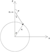 |
Fig. 1. Schematic of a photon emitted at the radiative shock, at height H above the surface of a neutron star of radius R, and hitting the surface. The polar angle of the photon is θ′ and the corresponding one at the point of incidence is θ. The relation between θ and θ′ is derived in the Appendix A. |
We assume a dipole magnetic field B with its dipole moment  along the z axis. The vector B on the surface of the neutron star of radius R is given by
![Mathematical equation: $$ \begin{aligned} {\boldsymbol{B}} = B_0 \left[3(\hat{m} \cdot \hat{r})\hat{r} -\hat{m} \right], \end{aligned} $$](/articles/aa/full_html/2021/11/aa39361-20/aa39361-20-eq3.gif) (2)
(2)
where B0 is the magnetic field at the equator of the neutron star and twice this at its pole,  is the radial unit vector, and
  is the unit vector along m. For a point in the xz plane, on the surface of the neutron star, we write
  , where θ is the polar angle, that is the angle between the radial vector and the z axis, and Eq. (2) becomes
![Mathematical equation: $$ \begin{aligned} {\boldsymbol{B}}(\theta ) = B_0 \left[(3 \cos ^2\theta -1) \hat{k} + 3 \cos \theta \sin \theta \;\hat{i} \right]. \end{aligned} $$](/articles/aa/full_html/2021/11/aa39361-20/aa39361-20-eq7.gif) (3)
(3)
The strength of the magnetic field on the surface of the neutron star at polar angle θ is
 (4)
(4)
The possibility of an off-center dipole exists, but it is beyond the present paper to investigate it. We have restricted ourselves to a centered dipole, as Poutanen et al. (2013) did.
Consider a photon emitted at the shock, at height H above the neutron-star surface, with direction  , in the xz plane. For angles θ′> π/2, such that sin θ′< R/(R + H), the photon will hit the neutron-star surface at a point (x, z), which is the intersection of the straight line path of the photon and the circle x2 + z2 = R2. The polar angle θ of this point (x, z), which will give the local magnetic field strength B(θ) (see Eq. (4)), is determined from either cos θ = z/R, z > 0 or sin θ = x/R, x > 0 (see Appendix A). We do not take into account gravitational bending, for two reasons. First, it is negligible. Using Eqs. (B.6) and (B.8) of Poutanen et al. (2013) and our Appendix A, we have found that for H = 10 km and m = 1 the magnetic field strength at the circumference of the illuminated polar cap is B = 0.69 B0 for the Newtonian case and B = 0.62 B0 when gravitational bending is taken into account. A ∼10% lower magnetic field has no effect in our conclusions. Second, gravitational bending brings the emitted photons at the radiative shock closer to the magnetic pole, and thus strengthens our main conclusion.
If  is the direction of a photon, then the angle of incidence with respect to the local magnetic field B(θ), at the first or any subsequent scattering, is determined from
 (5)
(5)
Here it is tacitly assumed that the region on the neutron-star surface sampled by the photon before it escapes is very small, i.e., the mean free path is much less than R, and B is constant in this region.
For a proper treatment of the radiative transfer, one needs to consider the complete, Quantum Electrodynamic, Compton cross sections (Herold 1979; Daugherty & Harding 1986; Harding & Daugherty 1991; Sina 1996; Gonthier et al. 2014; Mushtukov et al. 2016; Schwarm 2017). However, these cross sections are quite cumbersome, because they contain infinite sums, and are not very practical. A significant simplification of the above cross sections (though still intimidating) was derived by Nobili et al. (2008), in order to treat resonant scattering of photons with energy approaching mec2, in a magnetic field comparable to the critical one  . These cross sections were computed exactly at resonance, i.e., the Lorentz profile was approximated by a delta function.
Since most of the cyclotron lines that have been observed so far (Staubert et al. 2019) are at cyclotron energies ≪mec2, we restrict ourselves to resonant scattering of photons with energy E ≪ mec2 in a magnetic field of strength B ≪ Bcr. For such a case, we showed analytically and numerically (Loudas et al. 2021) that the modified classical cross sections given below in Eqs. (6a)–(6d) provide accurate representations of the fully relativistic ones.
For a cyclotron energy Ec(θ) = ℏωc(θ) = ℏeB(θ)/mec ≪ mec2, the modified classical polarization-dependent resonant cross sections are given by (Loudas et al. 2021)
 (6a)
(6a)
 (6b)
(6b)
 (6c)
(6c)
 (6d)
(6d)
where the index 1 (2) stands for the ordinary (extraordinary) mode, χ and χ′ are the incident and scattered angles, respectively, with respect to the local magnetic field, r0 is the classical electron radius, and c is the speed of light. The quantities L− and L+ are the normalized Lorentz profiles given by
 (7a)
(7a)
where ω and ωr are the photon frequency and the resonant frequency, respectively, in units of mec2/ℏ. The decay widths Γ± are given by Herold et al. (1982)
 (7b)
(7b)
 (7c)
(7c)
where α is the fine structure constant. We note that Γ− is equal to the classical  , which accounts for the finite transition life-time of the excited state (e.g., Daugherty & Ventura 1978; Ventura 1979).
The first terms in Eqs. (6a)–(6d) are the classical (Thomson) differential cross sections. The second terms, which are proportional to B/Bcr, are purely quantum mechanical and are due to spin flip. It is amazing that just these terms are enough to convert the classical cross sections into accurate approximations of the fully relativistic quantum-mechanical ones for B ≪ Bcr.
For the resonant frequency ωr and the new photon energy in the rest frame of the electron after scattering, we use Eqs. (8) and (6), respectively, of Nobili et al. (2008).
The polarization averaged differential cross section is given by
 (8)
(8)
For comparison, we have performed a calculation with this polarization averaged differential cross section.
The black-body temperature at the surface of the neutron star is typically ≲1 keV, which is much smaller than the cyclotron energy Ec = 25 keV at the pole, that we have considered, and one could consider the electrons at the surface of the neutron star as cold. However, the temperature of the electrons in the atmosphere of the neutron star can be up to an order of magnitude larger than the blackbody temperature (Zampieri et al. 1995). Thus, we have taken into account the temperature of the electrons. A one-dimensional (along the local B) nonrelativistic Maxwellian is fine for our purposes.
Since the heavy elements on the surface of the neutron star will not be completely ionized, for the absorption cross section, we use the hydrogenic approximation (Bethe & Salpeter 1957)
 (9)
(9)
where IZ = 13.6 Z2 eV is the ionization potential and we assume that the predominant element is Carbon (Z = 6). We remark that our conclusions are not affected at all if there are no heavy elements on the surface of the neutron star.
3. The Monte Carlo code
Our Monte Carlo code is similar to previously used codes in our work and it is based on Cashwell & Everett (1959) and Pozdnyakov et al. (1983). We emit photons toward the neutron star from height H, with a polar angle θ′, either in the form of a delta-function distribution or with continuous distributions given by Eq. (1) or that of Lyubarskii & Sunyaev (1988). The directions of emission are restricted between θ′=arcsin[R/(R + H)] (tangent) and θ′=π (pole).
We consider a uniform atmosphere at the surface of the neutron star, with the number density of the electrons ten times larger than the corresponding one for absorbers. This ratio of densities was selected so that absorption and scattering have comparable mean free paths at 15 keV. Below this energy, absorption dominates, while above it scattering dominates.
In our calculations, we consider a value for B0, such that Ec = 12.5 keV = 11.6 (B0/1 × 1012) keV at the equator and 25 keV at the pole. The variation of the strength of the magnetic field with polar angle θ is given by Eq. (4). Our input spectra have the form of a power law
 (10)
(10)
where E0 = 1 keV is a reference energy and α is the power-law index. For the Monte Carlo runs, we have used a minimum of 107 photons. For high resolution (e.g., Fig. 7), we have used 109 photons.
4. Results
As a test of our Monte Carlo code, and in order to see clearly the reflected spectrum, we first use a flat power-law spectrum as input, i.e., α = 0. For the photons to see a specific magnetic field strength, we send all of them to the pole, i.e., θ′=π. Equally well, we could have sent them to the tangent (θ′=arcsin[R/(R + H)]) or any intermediate direction. The temperature of the electrons is taken equal to zero, as a benchmark. In Fig. 2, we show our results. The black dashed line represents the input spectrum and the black crosses give the reflected spectrum. However, the observed spectra consist of two components: the photons that are emitted at the radiative shock and come directly to the observer and those that come to the observer after being reflected at the neutron-star surface. The relative strength of these two intensities is difficult to compute, because it depends on two angles, both unknown: the inclination of the spin axis of the neutron star and the angle between the spin and the magnetic axes. For most combinations of these two angles, the direct spectrum is more than 50% of the spectrum of the photons emitted at the radiative shock. Also, the larger the height H of the radiative shock, the larger the direct component. Therefore, in Fig. 2, we show mixtures of 50% direct and 50% reflected (blue stars) and 70% direct and 30% reflected (red pluses) as representative examples.
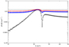 |
Fig. 2. Reflected spectrum dN/dE in all directions (black crosses) in arbitrary units, as a function of energy E in keV. The input spectrum is shown as a black dashed line. The other two lines show mixed spectra: 50% direct and 50% reflected (line with blue stars) and 70% direct and 30% reflected (line with red pluses). |
The reflected spectrum in Fig. 2 (black crosses) has the expected characteristics. First, the input photons near resonance have a small mean free path in the neutron-star atmosphere and, as a result, a good fraction of them get reflected. However, with every scattering these photons lose energy due to electron recoil. Thus, the reflected photons appear at energies below the resonance. Second, the resonant input photons that do not get reflected, but instead go deeper into the neutron-star atmosphere, face a large optical depth for escape and thus they escape only in the line wings. Similarly, photons with energy somewhat larger than Ec that go deep in the atmosphere, loose energy with every scattering and can escape, if they are not absorbed, only in the line wings. Thus, an absorption feature is generated at the resonance. However, since the atmosphere of the neutron star near resonance is an essentially pure scattering one, the number of photons is conserved. The photons that are missing in an absorption feature, must appear as an emission feature at lower energies, due to electron recoil.
At low energies, the reflected spectrum is significantly reduced due to absorption (see Eq. (9)). At high energies, the reduction of the reflected spectrum is due to down-scattering, followed by absorption.
Furthermore, we see in Fig. 2 that, despite the fact that the reflected spectrum has a sharp and prominent absorption feature, this feature is not so prominent when the reflected spectra are mixed with nonreflected ones, i.e., with input spectra that reach the observer directly. Naturally, the larger the direct component in the mixture, the shallower the absorption features and vice versa.
We repeated the calculation of Fig. 2, but with the polarization averaged differential cross section of Eq. (8), instead of the mode-dependent ones of Eqs. (6a)–(6d). The results are indistinguishable from those of Fig. 2.
In Fig. 3, we show the results of the same calculation, but with the thermal motion of the electrons taken into account. We consider values of kTe equal to 1 keV (line with black stars), 3 keV (line with blue circles), and 10 keV (line with red diamonds). The input spectrum is shown as a black dashed line.
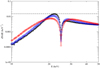 |
Fig. 3. Reflected spectrum dN/dE in all directions in arbitrary units, as a function of energy E in keV for kTe = 1 keV (line with black stars), kTe = 3 keV (line with blue circles), and kTe = 10 keV (line with red diamonds). The input spectrum is shown as a black dashed line. |
Contrary to our intuition regarding the thermal broadening of an absorption line, where the Lorentz profile is blue-shifted and red-shifted by the thermal motion of the absorbers, here the thermal motion of the electrons has a small and rather undetectable effect on the CRSF. The explanation is as follows.
Independent of the temperature of the electrons (assuming kTe ≲ 10 keV, as it is thought appropriate for a neutron star atmosphere), the discussion that we have given above for the formation of the absorption feature still holds. Photons at resonance cannot escape from deep in the atmosphere unless they change their energy and escape in the line wings. If the electrons are cold, resonance photons lose energy with every scattering and escape in the red wing. However, if the electrons are hot, they can give energy to the photons, which then escape in the blue wing. The hotter the electrons, the larger the blue wing. This is exactly what is seen in Fig. 3.
In the subsequent calculations and for concreteness, we take kTe = 1 keV, though the spectra are indistinguishable from those with kTe = 0. We stress that our conclusions are independent of the temperature of the electrons.
In Fig. 4, we show the dependesnce of the reflected spectrum on the direction of escape. The incident photons are again in the form of a pencil beam toward the pole. The line with the black circles gives the spectrum of the reflected photons that escape with angle χ′ with respect to the local  , such that 0 ≤ cos χ′< 0.33. The line with the blue diamonds corresponds to 0.33 ≤ cos χ′< 0.66 and the line with the red triangles corresponds to 0.66 ≤ cos χ′≤1.0. The three reflected spectra are very similar.
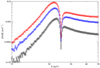 |
Fig. 4. Reflected spectrum dN/dE in three direction bins, as follows: 0 ≤ cos χ′< 0.33 (line with black circles), 0.33 ≤ cos χ′< 0.66 (line with blue diamonds), and 0.66 ≤ cos χ′≤1.0 (line with red triangles). The angle χ′ is measured with respect to B at the point of incidence. |
In Fig. 5, we use as input spectrum a steep power law with index α = 5, as suggested by the spectra in Tsygankov et al. (2006), Cusumano et al. (2016), and Doroshenko et al. (2017). Also, instead of dN/dE we show E2 dN/dE versus energy. The angle of incidence is θ′=π and the symbols are the same as in Fig. 2. The reflected spectrum has a prominent absorption feature, but in the mixed spectra (lines with stars and pluses) it is not as prominent.
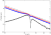 |
Fig. 5. Reflected spectrum in all directions in E2 dN/dE form (crosses), with arbitrary units, as a function of energy E in keV. The input spectrum is shown as a dashed line. The other two lines show mixed spectra: 50% direct and 50% reflected (stars) and 70% direct and 30% reflected (pluses). The angle θ′=π. |
In all of the above cases, we have considered a delta-function beam from the shock to the magnetic pole. However, as we have discussed in Sects. 2 and 3, the beam that is emitted at the shock is wide and it samples various magnetic field strengths on the surface of the neutron star. For a rather large shock height H = 10 km and R = 12.5 km, the beam extends from θ′=arcsin[R/(R + H)] = 146.3 degrees (tangent) to θ′ = 180 degrees (pole). At θ′ = 146.3 degrees, the photon hits the neutron-star surface at a polar angle (see Fig. 1) θ = 53.4 degrees (see Appendix A). The local magnetic field strength is B = 1.44 B0, with a corresponding cyclotron energy Ec = 17.97 keV.
In Fig. 6, we show the reflected spectra from a number of delta-function beams from θ′ = 147 degrees (grazing incidence) to θ′ = 180 degrees (vertical incidence) for a shock height H = 10 km. All delta-function beams have the same number of photons and their spectrum is that of the black dashed line. The red dotted line corresponds to θ′ = 147 degrees, with the local cyclotron energy Ec = 19.63 keV at the point of incidence. The green dot – dashed line corresponds to θ′ = 149 degrees (local Ec = 21.34 keV), the blue double-dot – dashed line corresponds to θ′ = 152 degrees (local Ec = 22.59 keV), the magenta double-dash – dotted line corresponds to θ′ = 155 degrees (local Ec = 23.33 keV), the black solid line corresponds to θ′ = 160 degrees (local Ec = 24.09 keV), and the brown long-dashed line corresponds to θ′ = 172 degrees (local Ec = 24.88 keV), As expected, the energy of the absorption feature increases with increasing θ′ from 17.97 keV to 25 keV.
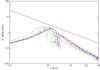 |
Fig. 6. Reflected spectra in all directions in E2 dN/dE form, with arbitrary units, as a function of energy E in keV. For all cases, the input spectrum is given by the black dashed line. The red dotted line corresponds to θ′ = 147 degrees, the green dot – dashed line corresponds to θ′ = 149 degrees, the blue double-dot – dashed line corresponds to θ′ = 152 degrees, the magenta double-dash – dotted line corresponds to θ′ = 155 degrees, the black solid line corresponds to θ′ = 160 degrees, and the brown long-dashed line corresponds to θ′ = 172 degrees. The corresponding energies of the cyclotron absorption features are given in the text. The shock height is H = 10 km. |
Two additional things are worth noticing in Fig. 6. (1) The absorption features are weaker when the photons have a grazing incidence in the atmosphere (θ′ = 147 degrees) than when they have a nearly perpendicular one (θ′ = 172 degrees). This is understood, because at grazing incidence the photons see a smaller absorption depth for escape than at normal incidence. (2) The absorption feature at grazing incidence (θ′ = 147 degrees) falls on top of the emission feature at incidence at θ′ = 149 degrees, and similarly for subsequent incidence angles. This has the important implication that when a beam falls on the neutron star, the addition of the reflected spectra, properly weighted with the angular distribution of the beam, will wash out the imprints of weaker magnetic fields from the low-magnetic-latitude part of the polar cap. We have found that this is indeed the case and this is the main point of our paper.
In Fig. 7, we show the reflected spectrum (red dot-dashed line) from an isotropic beam (m = 1 in Eq. (1)) and similarly (blue solid line) from a strongly beamed distribution (m = 3 in Eq. (1)). In both cases, the input spectrum is given by the black dashed line. The shock height is H = 5 km, which implies that, on the illuminated surface of the neutron star, Ec ranges from 20.0 to 25.0 keV. In both cases, the absorption feature from a broad beam is naturally wider than the corresponding one from a pencil beam (see Fig. 6). The minima, though, of the absorption features are at 24.7 keV for the m = 1 case and at 24.5 keV for the m = 3 case, which are very close to the cyclotron energy at the pole. The contribution of the lower magnetic latitudes is nearly washed out. The strongly beamed distribution (m = 3) produces an absorption feature (blue solid line in Fig. 7), which has slightly lower energy than that of the isotropic distribution (red line in Fig. 7, m = 1). This is because, in the m = 3 case, most of the photons hit the neutron-star surface at low magnetic latitudes and very few near the pole. We note that Fig. 7 shows only the reflected spectrum. The observed spectrum, however, is a combination of direct and reflected spectra, which makes the absorption features shallower (see Fig. 5).
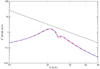 |
Fig. 7. Reflected spectra in all directions in E2 dN/dE form, with arbitrary units, as a function of energy E in keV. The red dot-dashed line corresponds to a beam with m = 1, while the blue solid line to a beam with m = 3. The shock height is H = 5 km and the input spectrum is given by the black dashed line. |
A shock height H = 5 km is rather large. We used it only for reasons of demonstration. In Fig. 8, we show the reflected spectrum of a beam with m = 1 and a reasonable shock height H = 2 km. A beam with m = 3 produces nearly identical results. The absorption feature occurs at the cyclotron energy corresponding to the magnetic field at the pole and, as expected, it is narrower than that of Fig. 7, because a narrower range of magnetic field strengths is sampled (22.74 ≤ Ec ≤ 25.0 keV). In the mixed spectra (stars and pluses), however, the absorption feature is less prominent.
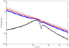 |
Fig. 8. Reflected spectrum (crosses) in all directions in E2 dN/dE form, with arbitrary units, as a function of energy E in keV. The photons are emitted in a beam with m = 1. The shock height is H = 2 km. The other two lines show mixed spectra: 50% direct and 50% reflected (stars) and 70% direct and 30% reflected (pluses). The input spectrum is given by the black dashed line. |
5. Comparison with observations
With regard to the change of the cyclotron-line energy with luminosity, the most remarkable X-ray pulsar to date is V 0332+53. It was demonstrated by Doroshenko et al. (2017) that, in its 2015 and 2016 outbursts, the cyclotron-line energy exhibited both a correlation (at low luminosities) and an anticorrelation (at high luminosities) with luminosity. Both, the correlation and the anticorrelation have been seen in other sources (for a review see Staubert et al. 2019), but todate this is the only source that exhibits both.
During the decay of the luminosity, the cyclotron-line energy increased from 27.9 keV to 30.4 keV. This is approximately a 9% increase.
To compare with these observations, we have run models with the shock height at H = 10, 8, 5, 3, and 1 km to mimic the decrease in the observed luminosity. We have also used a beam with m = 3, which is the most favorable to exhibit a variation of the cyclotron-line energy with shock height or equivalently luminosity. In Fig. 9 we show our results.
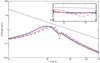 |
Fig. 9. Reflected spectra in all directions in E2 dN/dE form, with arbitrary units, as a function of energy E in keV for different shock heights: H = 10 km (black solid line), H = 8 km (blue dotted line), H = 5 km (red dashed line), H = 3 km (magenta dot-dashed line), and H = 1 km (green dash – dotted line). The dashed straight line is the input spectrum. The photons are emitted in a beam with m = 3. In the inset, we zoom into the absorption feature, with the horizontal axis linear. |
In varying the shock height by an order of magnitude, the cyclotron line varies from 24.5 ± 0.1 keV (the uncertainty is due to binning) to 25 keV, i.e., only about 0.2%. This is practically unobservable.
We remark that had we used a downward beam, most of the photons would hit the neutron-star surface near the magnetic pole and the variation of the cyclotron-line energy would be even smaller.
6. Discussion and conclusions
We have studied reflection of continuum X-ray photons from the surface of a magnetic neutron star. With a Monte Carlo code, we have simulated photons emitted from a radiative shock at height H above the surface of the neutron star, on the magnetic axis. The photons are either unidirectional or are in beams with specific distributions: isotropic, fan beam, or downward beam.
When the photons have a specific direction, they impinge in a polar ring on the neutron-star surface, that has a specific magnetic field. The lower the magnetic latitude of the ring, the lower the strength of the local dipole magnetic field. In such a case, the reflected spectrum exhibits a prominent cyclotron absorption line at the local cyclotron energy. Naturally, if the photons are emitted in a beam, a range of magnetic fields is sampled and the absorption line is wider.
If we could see only the reflected spectrum, these absorption features would be easily detectable. However, the observed X-ray spectra are a mixture of direct photons from the radiative shock and reflected ones. We have found that, for reasonable mixtures of direct and reflected photons, which depend on the inclination angle of the spin axis as well as on the angle between the magnetic and the spin axes (both unknown), the cyclotron features become much weaker than the ones observed (see, e.g., Fig. 3 of both Tsygankov et al. 2006; Doroshenko et al. 2017).
Another more serious finding, that speaks against the idea of cyclotron line formation at the surface of magnetic neutron stars, is that the reflected spectra are essentially unaffected by the height of the radiative shock. This is contrary to intuition, where one would expect an anticorrelation between the luminosity of the source, and therefore the height of the shock, and the cyclotron absorption feature (Poutanen et al. 2013). The reason for this is the following.
Consider photons at grazing incidence to the neutron-star surface. These photons impinge on the furthermost ring of the polar cap, which has the lowest magnetic field in the polar cap. Reflection of these photons creates (a) an absorption feature at the local cyclotron energy and (b) an emission feature below this. Consider now photons impinging on the adjacent ring, inside the first one. The strength of the magnetic field here is larger than that of the first ring. Thus, the emission feature at the local cyclotron energy falls on top of the absorption feature of the first ring, and the absorption feature is nearly washed out. The same thing happens with all inner rings. Since, in the illuminated polar cap, the magnetic field strength varies continuously from the circumference to the magnetic pole, illumination of the polar cap results in a broad cyclotron line, like the one shown in Fig. 7. The magnetic field inferred from such a line corresponds to that of the magnetic pole. We remark that the distribution of the photons in the beam is practically irrelevant. An isotropic beam and a strong fan beam give practically the same reflected spectrum. For this reason, we think that the use of gravitational bending will not alter the above picture.
Last, but not least, we remark that a shock height H = 10 km is unreasonably high. It was used only for the purpose of demonstration. For more reasonable heights of a few kilometers, the variation of the magnetic field in the polar cap is small and the spectra exhibit practically a broad absorption feature, which, in addition, is very shallow if the reflected spectra are mixed with direct ones. Thus, reflection at the surface of a neutron star is not the mechanism for cyclotron line formation.
Due to the overlap of the CRSFs at different magnetic-field strengths, reflection at the surface of a neutron star cannot explain the anticorrelation of cyclotron line energy and luminosity. Several alternative scenarios have been mentioned by Becker et al. (2012), Doroshenko et al. (2017), and Staubert et al. (2019), but a quantitative explanation of the effect is still pending.
Acknowledgments
N. D. K. would like to thank Sterl Phinney for his notes on the classical magnetic scattering cross sections.
References
- Araya, R., & Harding, A. 1999, ApJ, 517, 334 [NASA ADS] [CrossRef] [Google Scholar]
- Araya-Góchez, R., & Harding, A. 2000, ApJ, 544, 1067 [CrossRef] [Google Scholar]
- Basko, M. M., & Sunyaev, R. A. 1976, MNRAS, 175, 395 [Google Scholar]
- Becker, P. A., Klochkov, D., Schönherr, G., et al. 2012, A&A, 544, A123 [NASA ADS] [CrossRef] [EDP Sciences] [Google Scholar]
- Bethe, H. A., & Salpeter, E. E. 1957, Quantum Mechanics of One- and two-electron Systems (New York: Academic Press) [CrossRef] [Google Scholar]
- Cashwell, E. D., & Everett, C. J. 1959, A Practical Manual on the Monte Carlo Method for Random Walk Problems (New York: Pergamon Press) [Google Scholar]
- Cusumano, G., La Parola, V., D’Ai, A., et al. 2016, MNRAS, 460, L99 [NASA ADS] [CrossRef] [Google Scholar]
- Daugherty, J. K., & Harding, A. K. 1986, ApJ, 309, 362 [NASA ADS] [CrossRef] [Google Scholar]
- Daugherty, J. K., & Ventura, J. 1978, Phys. Rev. D, 18, 1053 [NASA ADS] [CrossRef] [Google Scholar]
- Doroshenko, V., Tsygankov, S. S., Mushtukov, A. A., et al. 2017, MNRAS, 466, 2143 [NASA ADS] [CrossRef] [Google Scholar]
- Fürst, F., Pottschmidt, K., Wilms, J., et al. 2014, ApJ, 780, 133 [Google Scholar]
- Gonthier, P. L., Baring, M. G., Eiles, M. T., et al. 2014, Phys. Rev. D, 90, 043014 [NASA ADS] [CrossRef] [Google Scholar]
- Harding, A. K., & Daugherty, J. K. 1991, ApJ, 374, 687 [NASA ADS] [CrossRef] [Google Scholar]
- Herold, H. 1979, Phys. Rev. D, 19, 2868 [NASA ADS] [CrossRef] [Google Scholar]
- Herold, H., Ruder, H., & Wunner, G. 1982, A&A, 115, 90 [NASA ADS] [Google Scholar]
- Kaminker, A. D., Fedorenko, V. N., & Tsygan, A. I. 1976, Sov. Astron., 20, 436 [NASA ADS] [Google Scholar]
- Klochkov, D., Staubert, R., Santangelo, A., et al. 2011, A&A, 532, A126 [NASA ADS] [CrossRef] [EDP Sciences] [Google Scholar]
- Klochkov, D., Doroshenko, V., Santangelo, A., et al. 2012, A&A, 542, L28 [NASA ADS] [CrossRef] [EDP Sciences] [Google Scholar]
- Kylafis, N. D., Trümper, J. E., & Ertan, Ü. 2014, A&A, 562, A62 [NASA ADS] [CrossRef] [EDP Sciences] [Google Scholar]
- La Parola, V., Cusumano, G., Segreto, A., & D’Ai, A. 2016, MNRAS, 463, 185 [NASA ADS] [CrossRef] [Google Scholar]
- Loudas, N. A., Kylafis, N. D., & Truemper, J. E. 2021, A&A, 655, A38 [NASA ADS] [CrossRef] [EDP Sciences] [Google Scholar]
- Lyubarskii, Y. E., & Sunyaev, R. A. 1988, Sov. Astron. Lett., 14, 390 [Google Scholar]
- Malacaria, C., Klochkov, D., Santangelo, A., & Staubert, R. 2015, A&A, 581, A121 [NASA ADS] [CrossRef] [EDP Sciences] [Google Scholar]
- Mitrofanov, I. G., & Tsygan, A. I. 1978, A&A, 70, 133 [NASA ADS] [Google Scholar]
- Mowlavi, N., Kreykenbohm, I., Shaw, S. E., et al. 2006, A&A, 451, 187 [NASA ADS] [CrossRef] [EDP Sciences] [Google Scholar]
- Mukherjee, D., & Bhattacharya, D. 2012, MNRAS, 420, 720 [NASA ADS] [CrossRef] [Google Scholar]
- Mushtukov, A. A., Tsygankov, S. S., Serber, A. V., Suleimanov, V. F., & Poutanen, J. 2015, MNRAS, 454, 2714 [Google Scholar]
- Mushtukov, A. A., Nagirner, D. I., & Poutanen, J. 2016, Phys. Rev. D, 93, 105003 [Google Scholar]
- Nagel, W. 1981, ApJ, 251, 288 [Google Scholar]
- Nishimura, O. 2008, ApJ, 672, 1127 [NASA ADS] [CrossRef] [Google Scholar]
- Nobili, L., Turolla, R., & Zane, S. 2008, MNRAS, 386, 1527 [NASA ADS] [CrossRef] [Google Scholar]
- Poutanen, J., Mushtukov, A. A., Suleimanov, V. F., et al. 2013, ApJ, 777, 115 [NASA ADS] [CrossRef] [Google Scholar]
- Pozdnyakov, L. A., Sobol, I. M., & Synyaev, R. A. 1983, Astrophys. Space Phys. Rev., 2, 189 [NASA ADS] [Google Scholar]
- Rothschild, R. E., Kühnel, M., Pottschmidt, K., et al. 2017, MNRAS, 466, 2752 [Google Scholar]
- Sartore, N., Jourdain, E., & Roques, J. P. 2015, ApJ, 806, 193 [NASA ADS] [CrossRef] [Google Scholar]
- Schönherr, G., Wilms, J., Kretschmar, P., et al. 2007, A&A, 472, 353 [NASA ADS] [CrossRef] [EDP Sciences] [Google Scholar]
- Schwarm, F. W. 2017, PhD Thesis, Friedrich-Alexander Universität, Germany [Google Scholar]
- Sina, R. 1996, PhD Thesis, University of Maryland, USA [Google Scholar]
- Staubert, R., Shakura, N. I., Postnov, K., et al. 2007, A&A, 465, L25 [NASA ADS] [CrossRef] [EDP Sciences] [Google Scholar]
- Staubert, R., Trümper, J. E., Kendziorra, E., et al. 2019, A&A, 622, A61 [NASA ADS] [CrossRef] [EDP Sciences] [Google Scholar]
- Trümper, J., Pietsch, W., Reppin, C., et al. 1977, Ann. N. Y. Acad. Sci., 302, 538 [CrossRef] [Google Scholar]
- Trümper, J., Pietsch, W., Reppin, C., et al. 1978, ApJ, 219, L105 [CrossRef] [Google Scholar]
- Trümper, J. E., Dennerl, K., Kylafis, N. D., et al. 2013, ApJ, 764, 49 [CrossRef] [Google Scholar]
- Tsygankov, S. S., Lutovinov, A. A., Churazov, E. M., & Sunyaev, R. A. 2006, MNRAS, 371, 19 [NASA ADS] [CrossRef] [Google Scholar]
- Tsygankov, S. S., Lutovinov, A. A., & Serber, A. V. 2010, MNRAS, 401, 1628 [NASA ADS] [CrossRef] [Google Scholar]
- Ventura, J. 1979, Phys. Rev. D., 19, 1684 [NASA ADS] [CrossRef] [Google Scholar]
- Ventura, J., Nagel, W., & Meszaros, P. 1979, ApJ, 233, L125 [NASA ADS] [CrossRef] [Google Scholar]
- Vybornov, V., Klochkov, D., Gornostaev, M., et al. 2017, A&A, 601, A126 [NASA ADS] [CrossRef] [EDP Sciences] [Google Scholar]
- Vybornov, V., Doroshenko, V., Staubert, R., & Santangelo, A. 2018, A&A, 610, A88 [NASA ADS] [CrossRef] [EDP Sciences] [Google Scholar]
- Zampieri, L., Turolla, R., Zane, S., & Treves, A. 1995, ApJ, 439, 849 [Google Scholar]
Appendix A: Geometry
We consider a point source on the magnetic axis z, at height H, above the surface of a neutron star. The source emits a pencil beam of photons with direction
in the xz plane, with the polar angle θ′> π/2 such that sin θ′≤R/(R + H). Under these conditions, the pencil beam hits the neutron-star surface at a point (x, z), which is determined from the intersection of the straight line
and the circumference of the circle

Eliminating z from these two equations we obtain

from which we get
and
where

and
The polar angle θ of the point (x, z) is determined from

All Figures
|
Fig. 1. Schematic of a photon emitted at the radiative shock, at height H above the surface of a neutron star of radius R, and hitting the surface. The polar angle of the photon is θ′ and the corresponding one at the point of incidence is θ. The relation between θ and θ′ is derived in the Appendix A. |
| In the text | |
|
Fig. 2. Reflected spectrum dN/dE in all directions (black crosses) in arbitrary units, as a function of energy E in keV. The input spectrum is shown as a black dashed line. The other two lines show mixed spectra: 50% direct and 50% reflected (line with blue stars) and 70% direct and 30% reflected (line with red pluses). |
| In the text | |
|
Fig. 3. Reflected spectrum dN/dE in all directions in arbitrary units, as a function of energy E in keV for kTe = 1 keV (line with black stars), kTe = 3 keV (line with blue circles), and kTe = 10 keV (line with red diamonds). The input spectrum is shown as a black dashed line. |
| In the text | |
|
Fig. 4. Reflected spectrum dN/dE in three direction bins, as follows: 0 ≤ cos χ′< 0.33 (line with black circles), 0.33 ≤ cos χ′< 0.66 (line with blue diamonds), and 0.66 ≤ cos χ′≤1.0 (line with red triangles). The angle χ′ is measured with respect to B at the point of incidence. |
| In the text | |
|
Fig. 5. Reflected spectrum in all directions in E2 dN/dE form (crosses), with arbitrary units, as a function of energy E in keV. The input spectrum is shown as a dashed line. The other two lines show mixed spectra: 50% direct and 50% reflected (stars) and 70% direct and 30% reflected (pluses). The angle θ′=π. |
| In the text | |
|
Fig. 6. Reflected spectra in all directions in E2 dN/dE form, with arbitrary units, as a function of energy E in keV. For all cases, the input spectrum is given by the black dashed line. The red dotted line corresponds to θ′ = 147 degrees, the green dot – dashed line corresponds to θ′ = 149 degrees, the blue double-dot – dashed line corresponds to θ′ = 152 degrees, the magenta double-dash – dotted line corresponds to θ′ = 155 degrees, the black solid line corresponds to θ′ = 160 degrees, and the brown long-dashed line corresponds to θ′ = 172 degrees. The corresponding energies of the cyclotron absorption features are given in the text. The shock height is H = 10 km. |
| In the text | |
|
Fig. 7. Reflected spectra in all directions in E2 dN/dE form, with arbitrary units, as a function of energy E in keV. The red dot-dashed line corresponds to a beam with m = 1, while the blue solid line to a beam with m = 3. The shock height is H = 5 km and the input spectrum is given by the black dashed line. |
| In the text | |
|
Fig. 8. Reflected spectrum (crosses) in all directions in E2 dN/dE form, with arbitrary units, as a function of energy E in keV. The photons are emitted in a beam with m = 1. The shock height is H = 2 km. The other two lines show mixed spectra: 50% direct and 50% reflected (stars) and 70% direct and 30% reflected (pluses). The input spectrum is given by the black dashed line. |
| In the text | |
|
Fig. 9. Reflected spectra in all directions in E2 dN/dE form, with arbitrary units, as a function of energy E in keV for different shock heights: H = 10 km (black solid line), H = 8 km (blue dotted line), H = 5 km (red dashed line), H = 3 km (magenta dot-dashed line), and H = 1 km (green dash – dotted line). The dashed straight line is the input spectrum. The photons are emitted in a beam with m = 3. In the inset, we zoom into the absorption feature, with the horizontal axis linear. |
| In the text | |
Current usage metrics show cumulative count of Article Views (full-text article views including HTML views, PDF and ePub downloads, according to the available data) and Abstracts Views on Vision4Press platform.
Data correspond to usage on the plateform after 2015. The current usage metrics is available 48-96 hours after online publication and is updated daily on week days.
Initial download of the metrics may take a while.