| Issue |
A&A
Volume 653, September 2021
|
|
|---|---|---|
| Article Number | L5 | |
| Number of page(s) | 7 | |
| Section | Letters to the Editor | |
| DOI | https://doi.org/10.1051/0004-6361/202141881 | |
| Published online | 15 September 2021 | |
Letter to the Editor
An unbiased NOEMA 2.6 to 4 mm survey of the GG Tau ring: First detection of CCS in a protoplanetary disk
1
Korea Astronomy and Space Science Institute, 776 Daedeokdae-ro, Yuseong-gu, Daejeon, Korea
e-mail: tpnguyen@kasi.re.kr
2
Department of Astrophysics, Vietnam National Space Center, Vietnam Academy of Science and Techonology, 18 Hoang Quoc Viet, Cau Giay, Hanoi, Vietnam
3
Laboratoire d’Astrophysique de Bordeaux, Université de Bordeaux, CNRS, B18N, Allée Geoffroy, Saint-Hilaire, 33615 Pessac, France
4
IRAM, 300 Rue de la piscine, 38406 Saint Martin d’Hères Cedex, France
5
Department of Physics and Astronomy, Colgate University, 13 Oak Drive, Hamilton, New York 13346, USA
6
Space Telescope Science Institute, 3700 San Martin Drive, Baltimore, Maryland 21218, USA
7
Institut de Recherche en Astrophysique et Planétologie, Université de Toulouse, UPS-OMP, CNRS, CNES, 9 Av. du Colonel Roche, 31028 Toulouse Cedex 4, France
8
Instituto de Ciencias Químicas Aplicadas, Facultad de Ingeniería, Universidad Autónoma de Chile, Av. Pedro de Valdivia 425, 7500912 Providencia, Santiago, Chile
9
School of Earth and Planetary Sciences, National Institute of Science Education and Research, HBNI, Jatni, 752050 Odisha, India
10
University of Science and Technology, 217 Gajeong-ro, Yuseong-gu, Daejeon 34113, Republic of Korea
11
Institut des Sciences Moléculaires, UMR5255-CNRS, 351 Cours de la libration, 33405 Talence, France
12
Academia Sinica Institute of Astronomy and Astrophysics, PO Box 23-141 Taipei 106, Taiwan
Received:
27
July
2021
Accepted:
27
August
2021
Context. Molecular line surveys are among the main tools to probe the structure and physical conditions in protoplanetary disks (PPDs), the birthplace of planets. The large radial and vertical temperature as well as density gradients in these PPDs lead to a complex chemical composition, making chemistry an important step to understand the variety of planetary systems.
Aims. We aimed to study the chemical content of the protoplanetary disk surrounding GG Tau A, a well-known triple T Tauri system.
Methods. We used NOEMA with the new correlator PolyFix to observe rotational lines at ∼2.6 to 4 mm from a few dozen molecules. We analysed the data with a radiative transfer code to derive molecular densities and the abundance relative to 13CO, which we compare to those of the TMC1 cloud and LkCa 15 disk.
Results. We report the first detection of CCS in PPDs. We also marginally detect OCS and find 16 other molecules in the GG Tauri outer disk. Ten of them had been found previously, while seven others (13CN, N2H+, HNC, DNC, HC3N, CCS, and C34S) are new detections in this disk.
Conclusions. The analysis confirms that sulphur chemistry is not yet properly understood. The D/H ratio, derived from DCO+/HCO+, DCN/HCN, and DNC/HNC ratios, points towards a low temperature chemistry. The detection of the rare species CCS confirms that GG Tau is a good laboratory to study the protoplanetary disk chemistry, thanks to its large disk size and mass.
Key words: astrochemistry / molecular data / protoplanetary disks / stars: individual: GG Tau A
© ESO 2021
1. Introduction
The chemical content in a protoplanetary disk (PPD) is thought to be a combination of parent cloud inheritances and the product of in situ reactions. PPDs are flared and layered, displaying important radial and vertical temperature and density gradients that result in a complex chemical structure and evolution. Each layer in the disk has conditions suitable for different chemical reactions, leading to different molecular abundances. For example, photo sensitive molecules such as CN and CCH are believed to probe the upper most layer which is directly irradiated by stellar UV; CO and its isotopologues arise from the layer just below it, while molecules are frozen on the dust grains (millimetre-sized) settled in the cold disk midplane. So far, more than thirty molecules have been detected in PPDs (see Phuong et al. 2018 for a list, and the more recent detections of H2CS by Le Gal et al. 2019, DNC by Loomis et al. 2020, SO by Rivière-Marichalar et al. 2020, and SO2 by Booth et al. 2021).
In this Letter, we report the first deep survey of a PPD covering the 2.6 to 4.2 mm window, where fundamental transitions of most simple molecules occur. We observed the GG Tau A system with the NOEMA interferometer. GG Tau A is a triple T Tauri system (Aa-Ab1/b2) with respective separations of 35 and 4.5 au (Di Folco et al. 2014), located in the Taurus-Auriga star forming region (150 pc, Gaia Collaboration 2018). It is surrounded by a large and massive Keplerian circumbinary (or ternary) disk with an estimated mass (Mdisk = 0.15 M⊙) using dust properties that are typically assumed for PPDs. The disk consists of a dense, narrow (radius from ∼180 to 260 au) ring that contains 70% of the disk mass. Beyond the ring, the outer gas disk extends out to ∼800 au. The temperature profile of the disk has been studied by Dutrey et al. (2014a), Guilloteau et al. (1999), and Phuong et al. (2020): the dust temperature is 14 K at 200 au, and the kinetic temperature derived from CO analysis is ∼25 K at the same radius. The large size, low temperature, and large mass make GG Tau A disk an ideal laboratory to study cold molecular chemistry.
We present the observations and results in Sect. 2. Data analysis using the radiative transfer code DiskFit is presented in Sect. 3. We then discuss the results in Sect. 4.
2. Observations and results
2.1. Observations
Observations were carried out using the NOEMA array between Sep. 2019 and Apr. 2020 (Projects S19AZ and W19AV). Four frequency setups were used to cover the frequency range 70.5−113.5 GHz. The PolyFix correlator covered the full bandwidth of ∼15 GHz at 2 MHz resolution (5−6.5 km s−1, while the total line width of GG Tau A is around 3.5 km s−1, see Fig. 1), plus a large number of spectral windows with a 62.5 kHz channel spacing (resolution 0.2−0.3 km s−1, comparable to the local thermal linewidth in GG Tau), optimised to cover a maximum number of spectral lines. The phase calibrators used were J0440+146 and 0507+179. Flux calibration was done using MWC349 and LkHa101. The standard pipeline in the CLIC package was used for calibration, with minor data editing. Three setups covering [70.5−78; 86−93.5], [80.5−88; 96−103.5], and [90.5−98; 106.3−113.5] GHz used the C and D configuration, while the band [88.8−96.5; 104.3−112] used the C and A configuration, providing enhanced sensitivity and angular resolution in the overlapping frequencies. In total, we covered at high spectral resolution of 70 rotational lines of 38 molecular species.
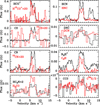 |
Fig. 1. Spectrum of each detected molecule, integrated in the area of 15″ × 15″ for lines with S/N > 5 and in the centre (central beam) of the detection area for lines with S/N < 5. Some lines have been scaled up by a factor (×x) to give a better view. |
2.2. Data reduction and imaging
We used the IMAGER1 interferometric imaging package to produce images. Continuum removal was carried out by the subtraction of a zero-order frequency baseline for each visibility in the uv plane. Various combinations of natural or robust weightings were used in the image processing to highlight the image properties. Beam sizes and sensitivities are summarised in Table 1 for all of the detected molecules. We note that HC3N and CCS have faint lines coming from similar rotational levels and similar line strengths: to illustrate their detection, lines from each molecule were stacked in velocity to produce a single data set. As synthesised beams exhibit significant sidelobes, deconvolution was done using the Hogbom method down to the rms noise. Integrated spectra are shown in Fig. 1, and moment 0 maps are shown in Figs. 2 and 3. To further enhance the S/N, we used the Keplerian deprojection technique using kinematics and geometrical parameters from Dutrey et al. (2014a), see Table 2. The images are deprojected and the velocities were corrected from the rotation pattern, thereby bringing all signals to the systemic velocity (see Teague et al. 2016; Yen et al. 2016). The resulting spectra and radius-velocity (RV) diagrams are shown in Figs. 4 and E.1. The ‘teardrop’ pattern (Teague 2019) expected for Keplerian disks transformed into ‘Eiffel tower’-like plots, because of the lack of emission from the tidal cavity of GG Tau A. Radial profiles of the line peak brightness are displayed in Appendix C.
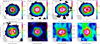 |
Fig. 2. From left to right, top to bottom: integrated intensity map of HCO+(1−0), CS(2−1), CN(1−0), HCN(1−0), HNC(1−0), N2H+, CCH, and H13CO+ (1−0). The white ellipses mark the approximate inner and outer edges of the dust ring at 180 au and 260 au, respectively. The beam size is indicated in the lower left corner and the colour scale is on the right is units of Jy beam−1 km s−1. The intensity was integrated in the velocity range from 4.0 to 9.0 km s−1 with the threshold of 3σ. Contour levels are spaced by 5σ in the maps of HCO+ and CS(2−1), and 3σ in the maps of CN, HCN, HNC, N2H+, CCH, and H13CO+ (1−0). |
Obtained beam and noise of detected molecules.
2.3. Results
Among the 38 molecules which were observed in the survey, 17 are detected, including 13CO and C18O, which we do not present in this Letter. The high resolution maps of these two molecules can be found in Phuong et al. (2020).
The CN, HCN, HNC, HCO+, CS, N2H+, and CCH lines were detected at high S/N, as it can be seen in Fig. 2. All lines appear optically thin, as illustrated by the hyperfine ratios of HCN, CN, CCH, and N2H+ (see Fig. E.1), and also by the peak brightness of HCO+ (5.5 K).
Some molecules observed with a sufficiently high angular resolution (HCO+, HCN, and N2H+) display a clear east-west asymmetry. In a tilted Keplerian disk, the maximum opacity was obtained along the major axis, resulting in two symmetric peaks. The observed asymmetry is most obvious in HCO+, suggesting that it is related to the ‘hot spot’ detected at PA 120° (Dutrey et al. 2014a; Tang et al. 2016; Phuong et al. 2020). Furthermore, CCH may also be enhanced there, while the HNC map suggests a (marginal) deficit at this position.
The apparent peak towards GG Tau for CN and CS emission is due to the lower angular resolution of these data. Their RV diagrams (Figs. 4 and E.1) clearly show that no emission is coming from inside about 200 au.
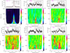 |
Fig. 4. Integrated spectra (with Gaussian fits in red and fit results are indicated) and radial-velocity diagram of CS, C34S(2−1), CCS, 13CS(2−1), 13CN, and DNC obtained after making a Keplerian velocity correction. |
As is shown in Figs. 2–4, H13CO+, para-H2CO, HC3N, and C34S molecules have been detected with moderate S/N. The RV diagrams show that H13CO+ and N2H+ are more prominent in the dense ring, while CCH and H2CO come only from the outer disk, beyond 300 au out to about 600 au (see Fig. E.1). The non-detection of the o-H2CO 6(1, 5) − 6(1, 6) transition is consistent with the expected temperature and an ortho-para ratio of 3.
The DNC, 13CS, 13CN, and CCS lines have been detected at low S/N (∼6−8σ). Since the data are very noisy, in Fig. 4, we have chosen to only present their integrated spectra (top) and the RV diagram (bottom) obtained after Keplerian velocity correction, which best illustrate the detectability.
Regarding the undetected molecules list, we may have marginal detections (∼2−3σ) of OCS, and perhaps DCO+ and DCN. However, could not detect 13C17O, N2D+, H13CN, HC15N, HN13C, H15NC, HOC+, HCNH+, HCCCHO, SO, SO2, H2CS, SiO, CCD, HDO, D2CO, c-C3H2, or CH3CN molecules.
3. Radiative transfer modelling with DiskFit
The data were compared in the uv-plane with visibilities predicted for a disk model using the radiative transfer code DiskFit (Piétu et al. 2007). A description of DiskFit usage for GG Tau can be found in the appendix of Phuong et al. (2020).
The geometric parameters (inclination, orientation) and the physical power laws (velocity and temperature), derived from previous papers, are given in Table 2. As in Phuong et al. (2018), we kept the velocity and temperature laws as well as the power index (p = 1.5) of the molecular surface density fixed. Only Σ250, the value of the molecular surface density at 250 au, was left free and varied during the minimisation process.
GG Tau parameters.
We assumed that all molecules, except sulphur-bearing species, arise from the same layer as CO, so that they share the same temperature profile, T(r) = 25 (r/200 au)−1.0 K. Following Dutrey et al. (2017) on the Flying Saucer edge-on disk, CS arises from the lower part of the molecular layer, closest to the disk midplane. We thus decided to analyse sulphur-bearing species with a lower temperature, namely the temperature profile derived from dust emission at millimetre wavelengths (T(r) = 15 (r/200 au)−1.0 K, Dutrey et al. 2014a). Because optically thin 1−0 line intensities scale roughly as Σ/T above 10 K, the temperature spread due to the specific molecular layer can only affect the derived surface density by a factor of 2 at most. The factor is even smaller for heavier molecules such as CCS, HC3N, and OCS, since the observed lines are close to the brightest ones expected at these temperatures. The molecular surface densities are given in Table 3, with 3σ upper limits for non-detections. Assuming an exponent p = 1 only changes the surface densities by less than 30% (see Table B.1).
Molecular surface density at 250 au derived with DiskFit.
4. Discussion
4.1. Sulphur in protoplanetary disk: First detection of CCS
Beyond CS, only a few S-bearing species observed in molecular clouds are detected in disks: H2S (Phuong et al. 2018), H2CS (Le Gal et al. 2019), SO (Rivière-Marichalar et al. 2020), and SO2 (although in a very atypical, warm disk, Booth et al. 2021). In the GG Tau ring, we detected CCS, 13CS, and C34S but failed to detect H2CS, SO, and SO2. Though OCS may be marginally detected, however (see appendix).
The CCS surface density measured in the GG Tau ring, (1.5 ± 0.2) × 1012 cm−2, is of the order of the best previously reported upper limits in TTS and HAe disks. Using the IRAM array, Chapillon et al. (2012) reported upper limits (at 300 au) of (0.9 − 1.4) × 1012 cm−2 in LkCa 15, GO Tau, DM Tau, and MWC 480 disks, while Le Gal & MAPS Collaboration (2021) through the ALMA Large Program MAPs, obtained limits in the range 1012 − 1013 cm−2 for IM Lup, GM Aur, AS 209, HD 163296, and MWC 480 disks. It is also consistent with our previous upper limit of < 1.7 × 1012 cm−2 in GG Tau (Phuong et al. 2018).
Using Nautilus, a three phase gas-grain chemical model (Ruaud et al. 2016), Phuong et al. (2018) modelled the chemistry in the GG Tau ring. They predicted a CCS surface density of 7.2 × 1010 cm−2 at 250 au, a factor 20 lower than the observed value. Our new upper limits of SO and SO2 are comparable with the previous ones and are still in reasonable agreement with the chemical model presented in Phuong et al. (2018). This model is also compatible with our detection of HC3N, which was not detected by Phuong et al. (2018). However, for H2S, Phuong et al. (2018) predicted a surface density of 3.4 × 1013 cm−2 a factor 100 larger than what was observed. They conclude that H2S is likely transformed in more complex species at grain surfaces, precluding any thermal desorption. The failure to predict CCS further supports the idea of an incomplete handling of the complex sulphur chemistry in disk chemical models, in addition to the difficulty of estimating the amount of sulphur depletion in refractory materials in grains prior to disk formation.
4.2. Comparison with TMC1 and LkCa15
Table 4 is a comparison of molecular abundances relative to 13CO with the TMC1 dark cloud and the transition disk (cavity of radius 50 au Piétu et al. 2007) of LkCa 15, a T Tauri star with a disk mass ∼0.028 M⊙ (Guilloteau et al. 2011). For GG Tau A, we used a 13CO column density of Σ250 = 1.1 × 1016 cm−2 (Phuong et al. 2020), while for LkCa 15 we used ≃3.6 × 1015 cm−2 (Piétu et al. 2007).
Molecular abundance with respect to 13CO: 105 × (Xmol/X13CO).
For TMC-1, we used ∼1.1 × 1016 cm−2, following Cernicharo et al. (2021). Relative abundances were then calculated using different studies. At first order, these abundances (and the observed D/H ratios, see Appendix A) suggest that the GG Tau and LkCa 15 disks share similar chemical properties. We note however that the radical abundances (CN and CCH) are somewhat lower towards GG Tau, perhaps because the GG Tau dense ring is shadowing the outer disk, reducing the UV flux.
Sulphur-bearing species. The CS/C34S ratio, 25 ± 3, is compatible with solar isotopic ratios and optically thin CS (2−1) emission. Despite limited S/N, the CCS emission (Fig. 4) seems to arise from the dense ring, as for H2S (Phuong et al. 2018). We find that CS/CCS ∼17 is similar to the CS/H2S ratio (Phuong et al. 2018), and somewhat higher than the value reported in TMC1 (∼6.3, Cernicharo et al. 2021). Moreover, we observe 13CS/12CS ≃ 0.01, while Le Gal et al. (2019) found 0.015 in LkCa 15.
CCS can form via three routes. The first route being S++C2H2 → HCCS++H and HCCS++e → CCS+H and the second one being CCH+S → CCS+H, which are exothermic and free of reaction barriers, play important roles in the sulphur chemistry in molecular clouds, while the third route CH+CS → CCS+H is the main production pathway. Sakai et al. (2007) reported 13CCS/C13CS ∼ 4 in TMC-1 and L1521E, indicating that the two carbon atoms making up CCS are not equivalent and have to come from different molecular species or non-equivalent positions of a single molecule (e.g. HC3N, CCH, c-C3H2, C3S, and C4H, Takano et al. 1990; Sakai et al. 2010a,b; Yoshida et al. 2015). After formation, CCS can be a precursor of CS via several reactions (Vastel et al. 2018; Semenov et al. 2018). In the outer region of a protoplanetary disk, the sulphur chemistry starts with the S+ ion, the least efficient formation route of CCS. This probably makes the molecule in PPDs much less abundant than in molecular clouds.
The angular resolution of these data is insufficient for proper comparisons with a chemical model and the determination of radial variations, although physical conditions in the dense ring and the outer disk are known to be different (Phuong et al. 2020). Such comparisons would require high angular resolution images, but this is a challenging task given the low frequencies at which heavy molecules such as CCS or OCS have their peak emission at temperatures of 15−25 K or below. Nevertheless, the detection of a new rare species, CCS, in the dense ring of GG Tau confirms it is a good laboratory to study the cold PPD chemistry, thanks to its large size and mass.
Acknowledgments
This work is based on observations carried out with the IRAM NOEMA Interferometer. IRAM is supported by INSU/CNRS (France), MPG (Germany) and IGN (Spain). A. Dutrey and S. Guilloteau thank the French CNRS programs PNP, PNPS and PCMI. N. T. Phuong and P. N. Diep acknowledge financial support from World Laboratory, Rencontres du Viet Nam, and Vietnam National Space Center. N. T. Phuong thanks financial support from Korea Astronomy and Space Science Institute. This research is funded by Vietnam National Foundation for Science and Technology Development (NAFOSTED) under grant number 103.99-2019.368. A. C. acknowledges financial support from the Agence Nationale de la Recherche (grant ANR-19-ERC7-0001-01). C. W. L. is supported by the Basic Science Research Program through the National Research Foundation of Korea (NRF) funded by the Ministry of Education, Science and Technology (NRF-2019R1A2C1010851).
References
- Aikawa, Y., Furuya, K., Hincelin, U., & Herbst, E. 2018, ApJ, 855, 119 [CrossRef] [Google Scholar]
- Bergin, E. A., Cleeves, L. I., Gorti, U., et al. 2013, Nature, 493, 644 [NASA ADS] [CrossRef] [PubMed] [Google Scholar]
- Booth, A. S., van der Marel, N., Leemker, M., van Dishoeck, E. F., & Ohashi, S. 2021, A&A, 651, L6 [NASA ADS] [CrossRef] [EDP Sciences] [Google Scholar]
- Butner, H. M., Lada, E. A., & Loren, R. B. 1995, ApJ, 448, 207 [NASA ADS] [CrossRef] [Google Scholar]
- Cernicharo, J., Cabezas, C., Agúndez, M., et al. 2021, A&A, 648, L3 [EDP Sciences] [Google Scholar]
- Chapillon, E., Dutrey, A., Guilloteau, S., et al. 2012, ApJ, 756, 58 [NASA ADS] [CrossRef] [Google Scholar]
- Di Folco, E., Dutrey, A., Le Bouquin, J.-B., et al. 2014, A&A, 565, L2 [NASA ADS] [CrossRef] [EDP Sciences] [Google Scholar]
- Dutrey, A., Guilloteau, S., & Guelin, M. 1997, A&A, 317, L55 [NASA ADS] [Google Scholar]
- Dutrey, A., di Folco, E., Guilloteau, S., et al. 2014a, Nature, 514, 600 [NASA ADS] [CrossRef] [Google Scholar]
- Dutrey, A., Semenov, D., Chapillon, E., et al. 2014b, in Protostars and Planets VI, eds. H. Beuther, R. S. Klessen, C. P. Dullemond, & T. Henning, 317 [Google Scholar]
- Dutrey, A., Guilloteau, S., Piétu, V., et al. 2017, A&A, 607, A130 [NASA ADS] [CrossRef] [EDP Sciences] [Google Scholar]
- Gaia Collaboration (Brown, A. G. A., et al.) 2018, A&A, 616, A1 [NASA ADS] [CrossRef] [EDP Sciences] [Google Scholar]
- Guilloteau, S., Dutrey, A., & Simon, M. 1999, A&A, 348, 570 [NASA ADS] [Google Scholar]
- Guilloteau, S., Dutrey, A., Piétu, V., & Boehler, Y. 2011, A&A, 529, A105 [NASA ADS] [CrossRef] [EDP Sciences] [Google Scholar]
- Guilloteau, S., Reboussin, L., Dutrey, A., et al. 2016, A&A, 592, A124 [NASA ADS] [CrossRef] [EDP Sciences] [Google Scholar]
- Huang, J., Öberg, K. I., Qi, C., et al. 2017, ApJ, 835, 231 [NASA ADS] [CrossRef] [Google Scholar]
- Le Gal, R., & MAPS Collaboration 2021, ApJS, submitted [Google Scholar]
- Le Gal, R., Öberg, K. I., Loomis, R. A., Pegues, J., & Bergner, J. B. 2019, ApJ, 876, 72 [Google Scholar]
- Liszt, H. S., & Ziurys, L. M. 2012, ApJ, 747, 55 [Google Scholar]
- Loomis, R. A., Öberg, K. I., Andrews, S. M., et al. 2020, ApJ, 893, 101 [CrossRef] [Google Scholar]
- Omont, A. 2007, Rep. Progr. Phys., 70, 1099 [Google Scholar]
- Phuong, N. T., Chapillon, E., Majumdar, L., et al. 2018, A&A, 616, L5 [NASA ADS] [CrossRef] [EDP Sciences] [Google Scholar]
- Phuong, N. T., Dutrey, A., Diep, P. N., et al. 2020, A&A, 635, A12 [CrossRef] [EDP Sciences] [Google Scholar]
- Piétu, V., Dutrey, A., & Guilloteau, S. 2007, A&A, 467, 163 [NASA ADS] [CrossRef] [EDP Sciences] [Google Scholar]
- Qi, C., Kessler, J. E., Koerner, D. W., Sargent, A. I., & Blake, G. A. 2003, ApJ, 597, 986 [NASA ADS] [CrossRef] [Google Scholar]
- Rivière-Marichalar, P., Fuente, A., Le Gal, R., et al. 2020, A&A, 642, A32 [EDP Sciences] [Google Scholar]
- Ruaud, M., Wakelam, V., & Hersant, F. 2016, MNRAS, 459, 3756 [NASA ADS] [CrossRef] [Google Scholar]
- Sakai, N., Ikeda, M., Morita, M., et al. 2007, ApJ, 663, 1174 [NASA ADS] [CrossRef] [Google Scholar]
- Sakai, N., Saruwatari, O., Sakai, T., Takano, S., & Yamamoto, S. 2010a, A&A, 512, A31 [NASA ADS] [CrossRef] [EDP Sciences] [Google Scholar]
- Sakai, N., Shiino, T., Hirota, T., Sakai, T., & Yamamoto, S. 2010b, ApJ, 718, L49 [NASA ADS] [CrossRef] [Google Scholar]
- Semenov, D., Favre, C., Fedele, D., et al. 2018, A&A, 617, A28 [NASA ADS] [CrossRef] [EDP Sciences] [Google Scholar]
- Takano, S., Suzuki, H., Ohishi, M., et al. 1990, ApJ, 361, L15 [NASA ADS] [CrossRef] [Google Scholar]
- Tang, Y.-W., Dutrey, A., Guilloteau, S., et al. 2016, ApJ, 820, 19 [NASA ADS] [CrossRef] [Google Scholar]
- Teague, R. 2019, J. Open Sour. Softw., 4, 1632 [NASA ADS] [CrossRef] [Google Scholar]
- Teague, R., Guilloteau, S., Semenov, D., et al. 2016, A&A, 592, A49 [NASA ADS] [CrossRef] [EDP Sciences] [Google Scholar]
- Turner, B. E. 2001, ApJS, 136, 579 [Google Scholar]
- van Dishoeck, E. F., Thi, W.-F., & van Zadelhoff, G.-J. 2003, Ap&SS, 285, 691 [NASA ADS] [CrossRef] [Google Scholar]
- Vastel, C., Quénard, D., Le Gal, R., et al. 2018, MNRAS, 478, 5514 [Google Scholar]
- Yen, H.-W., Koch, P. M., Liu, H. B., et al. 2016, ApJ, 832, 204 [NASA ADS] [CrossRef] [Google Scholar]
- Yoshida, K., Sakai, N., Tokudome, T., et al. 2015, ApJ, 807, 66 [Google Scholar]
Appendix A: Deuterated species
All D/H ratios (Fig. A.1) are very similar (within the error bars) and around 0.01-0.05. As already quoted by several studies, such values are in agreement with dark cloud measurements and consistent with a low temperature chemistry (e.g. Phuong et al. 2018; van Dishoeck et al. 2003; Bergin et al. 2013; Dutrey et al. 2014b; Huang et al. 2017; Aikawa et al. 2018).
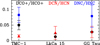 |
Fig. A.1. D/H ratios in TMC-1, LkCa 15, and GG Tau A. |
Appendix B: Molecular surface density derived with power index of p = 1.0 for surface density law
Molecular surface density at 250 au assuming p = 1.
Appendix C: Radial profiles
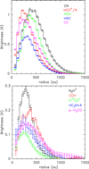 |
Fig. C.1. Radial profiles of brightness temperature at systemic velocity of 6.4 km s−1 of molecular lines detected at SNR> 5. |
Appendix D: Radial-velocity diagram of OCS
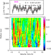 |
Fig. D.1. Integrated spectra (top) and radial-velocity diagram (bottom) of OCS obtained after making a Keplerian velocity correction and line stacking. |
Appendix E: Radial-velocity diagrams of other detected molecules
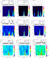 |
Fig. E.1. Top: Integrated spectra of CN, HCO+, HCN, N2H+, HNC, CCH, H13CO+, H2CO, and HC3N (with Gaussian fits, including hyperfine structure when needed, in red). The values indicate the fit results. Bottom: Corresponding radial-velocity diagram obtained after making Keplerian velocity correction and line stacking. |
All Tables
All Figures
|
Fig. 1. Spectrum of each detected molecule, integrated in the area of 15″ × 15″ for lines with S/N > 5 and in the centre (central beam) of the detection area for lines with S/N < 5. Some lines have been scaled up by a factor (×x) to give a better view. |
| In the text | |
|
Fig. 2. From left to right, top to bottom: integrated intensity map of HCO+(1−0), CS(2−1), CN(1−0), HCN(1−0), HNC(1−0), N2H+, CCH, and H13CO+ (1−0). The white ellipses mark the approximate inner and outer edges of the dust ring at 180 au and 260 au, respectively. The beam size is indicated in the lower left corner and the colour scale is on the right is units of Jy beam−1 km s−1. The intensity was integrated in the velocity range from 4.0 to 9.0 km s−1 with the threshold of 3σ. Contour levels are spaced by 5σ in the maps of HCO+ and CS(2−1), and 3σ in the maps of CN, HCN, HNC, N2H+, CCH, and H13CO+ (1−0). |
| In the text | |
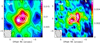 |
Fig. 3. Same as Fig. 2, but for H2CO and HC3N, respectively. The contour levels are spaced by 2σ. |
| In the text | |
|
Fig. 4. Integrated spectra (with Gaussian fits in red and fit results are indicated) and radial-velocity diagram of CS, C34S(2−1), CCS, 13CS(2−1), 13CN, and DNC obtained after making a Keplerian velocity correction. |
| In the text | |
|
Fig. A.1. D/H ratios in TMC-1, LkCa 15, and GG Tau A. |
| In the text | |
|
Fig. C.1. Radial profiles of brightness temperature at systemic velocity of 6.4 km s−1 of molecular lines detected at SNR> 5. |
| In the text | |
|
Fig. D.1. Integrated spectra (top) and radial-velocity diagram (bottom) of OCS obtained after making a Keplerian velocity correction and line stacking. |
| In the text | |
|
Fig. E.1. Top: Integrated spectra of CN, HCO+, HCN, N2H+, HNC, CCH, H13CO+, H2CO, and HC3N (with Gaussian fits, including hyperfine structure when needed, in red). The values indicate the fit results. Bottom: Corresponding radial-velocity diagram obtained after making Keplerian velocity correction and line stacking. |
| In the text | |
Current usage metrics show cumulative count of Article Views (full-text article views including HTML views, PDF and ePub downloads, according to the available data) and Abstracts Views on Vision4Press platform.
Data correspond to usage on the plateform after 2015. The current usage metrics is available 48-96 hours after online publication and is updated daily on week days.
Initial download of the metrics may take a while.