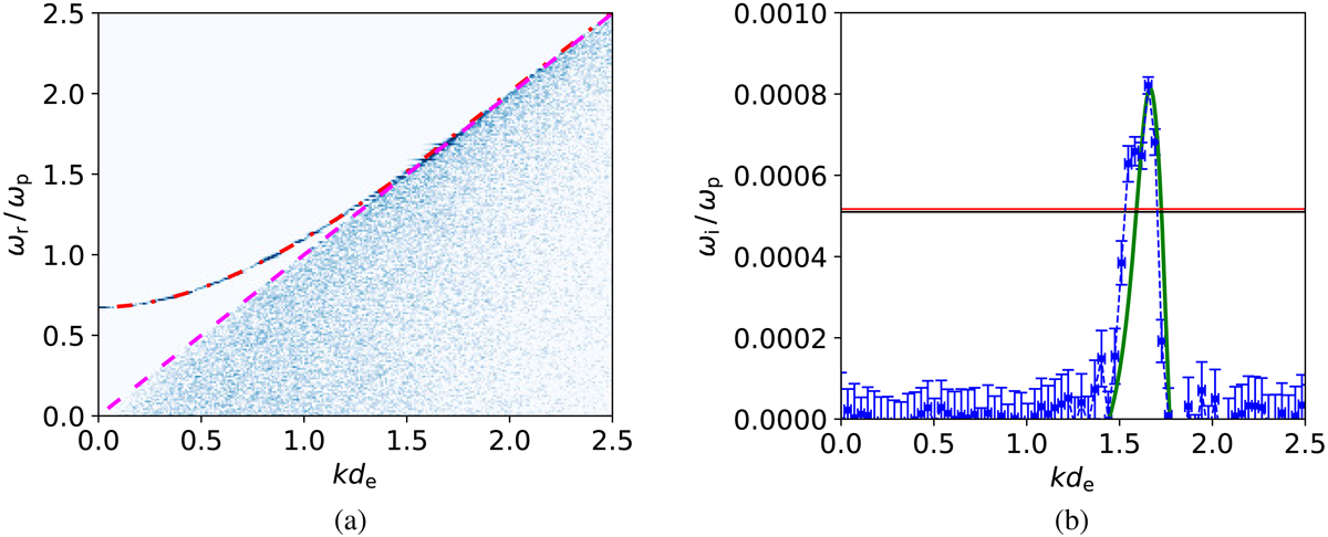
Comparison between a solution obtained by linear theory with the one from simulation for ρ₀ = ρ₁ = 1, γ_b = 26, r_n = 10⁻³. Panel a: dispersion diagram showing the real part of the frequency ω_r as a function of the wavevector k. The background in blue colour scale represents the power spectral density obtained from the simulation electric field E(x, t). The discontinuous lines represent solutions of the linear dispersion relation Eq. (1): the superluminal L-mode branch (dash-dotted red line) and the subluminal branch (dashed magenta line). Panel b: imaginary part of the frequency ω_i (corresponding to the growth rates) as a function of the wavenumber k for the subluminal branch. The green line shows the solution of the linear dispersion relation, and the dashed blue lines with error bars indicate the simulation results. The horizontal lines represent the values of the integrated growth rates obtained from the dispersion relation (red line) and from the simulation (black line).