| Issue |
A&A
Volume 647, March 2021
|
|
|---|---|---|
| Article Number | A155 | |
| Number of page(s) | 8 | |
| Section | Atomic, molecular, and nuclear data | |
| DOI | https://doi.org/10.1051/0004-6361/202039790 | |
| Published online | 26 March 2021 | |
Rate coefficients for H2:H2 inelastic collisions in the ground vibrational state from 10 to 1000 K★
1
Instituto de Física Fundamental, CSIC (IFF-CSIC),
C/ Serrano 123,
28006
Madrid,
Spain
e-mail: This email address is being protected from spambots. You need JavaScript enabled to view it.
2
Laboratory of Molecular Fluid Dynamics, Instituto de Estructura de la Materia, CSIC (IEM-CSIC),
C/ Serrano 121,
28006
Madrid,
Spain
e-mail: This email address is being protected from spambots. You need JavaScript enabled to view it.
Received:
29
October
2020
Accepted:
25
January
2021
Abstract
Aims. In this work, we present a pruned set of state-to-state rate coefficients (STS rates) for inelastic H2:H2 collisions in the thermal range from 10 to 1000 K. The set includes all relevant rates needed for diagnostics based on the simulation of quadrupole infrared spectra of H2.
Methods. The reported set was obtained from a quantum scattering close-coupling calculation employing a recent version of the MOLSCAT code, a high-level potential energy surface, and rotational energies of the H2 molecules with spectroscopic accuracy. These improvements have led to a significant increase in the accuracy with respect to previous computational results. The accuracy of the present STS rates is tested against recently reported experimental rates. Most dominant rates agree with the experiment within a 2σ uncertainty (2 to 6%).
Results. In addition to the tables given in the main text, three machine-readable tables are available at the CDS. These tables include all the relevant numerical results of the paper, namely, the excitation and de-excitation STS rates for H2:H2 inelastic collisions at selected temperatures between 10 and 1000 K, and their functional description for interpolation at any intermediate temperature.
Key words: molecular processes
Full Table 1 and Tables 2 and 3 are available at the CDS via anonymous ftp to cdsarc.u-strasbg.fr (130.79.128.5) or via http://cdsarc.u-strasbg.fr/viz-bin/cat/J/A+A/647/A155
© ESO 2021
1 Introduction
As the most abundant and ubiquitous stable molecular species in the universe, H2 has been the subject of a great number of observational works in recent decades (Dalgarno 2000; Habart et al. 2005; Huestis 2008). In particular, the infrared quadrupole emission following the decay from ultraviolet absorption in H2-rich regions of the universe has provided a useful diagnostics tool based on the analysis of the infrared emission spectra (Black & van Dishoeck 1987; Sternberg & Dalgarno 1989). The line intensities of these spectra are given by
 (1)
(1)
where vj and v′j′ are the vib-rotational quantum numbers of the upper and lower energy levels of the transition, A is the quadrupole radiative transition probability, ν is the transition frequency, and Nvj is the total column density of pumped molecules in level vj.
Modelling of H2-rich regions of the interstellar medium rests upon the solution of the system of level population-destruction equations (Black & van Dishoeck 1987; Sternberg &Dalgarno 1989), where the number densities of the molecular and atomic participants combine with the quadrupole transition probabilitiesA(vj → v′j′) and with other physical quantities relevant for the statistical equilibrium. These ingredients include, among others, the temperature dependent collision state-to-state rate coefficients, Q(T; vj → v′j′) (STS rates in short), and the UV excitation rates, P(vj → v*j*), which depend on the UV field intensity and on the number density of atomic and molecular hydrogen species.
Simulation of the observed IR emission spectra under the constraints of the population-destruction equations leads to the modelling of the H2 medium, producing quantitative information on temperatures, densities, UV radiation field, and the ortho-H2 (oH2) to para-H2 (pH2) ratio. Among the various ingredients needed for this procedure the most elusive ones are the Q(T; vj → v′j′) STS rates. The quadrupole (electric and magnetic) and dipole (magnetic) transition probabilities are accurately established (Roueff et al. 2019), while the UV pumping rates P(vj → v*j*) are subject to a number of physical uncertainties. Other applications of the STS rates in astrophysical environments concern the low-density-limit cooling function Λ(T) as a function of temperature for the various H2 :H2 inelastic collision processes (Lee et al. 2008).
The Q(T;vj → v′j′) STS rates for collisions involving hydrogen species have been the subject of a great number of theoretical and computational works in theframe of the quantum scattering theory, but just a few experimental works have been reported. In spite of this effort, only partial results of uncertain accuracy have been available until recently. Relatively complete sets of calculated Q(T; vj → v′j′) STS rates for H2 :H2 inelastic collisions in the v = 0 ground state of H2 based on high-quality H2 -H2 intermolecular potential energy surfaces (PES) were reported by Montero et al. (2006) and Montero & Pérez-Ríos (2014) employing the rigid-rotor DJ00-PES by Diep & Johnson (2000).
The following partial results on STS rates for inelastic H2 :H2 collisions within v = 0 vibrational state are discussed below: the FR98 set (Flower & Roueff 1998, 1999) based on Sw88-PES (Schwenke 1988); the Lee08 set (Lee et al. 2008) based on DJ00-PES (Diep & Johnson 2000); and the Wan18 set (Wan et al. 2018; Stancil, priv. comm.) based on P08-PES (Patkowski et al. 2008). The FR98 set can also be retrieved from the BASECOL 2012 database (Dubernet et al. 2013), and the Lee08 set from the UGAMOP database (Lee et al. 2008).
These three sets of STS rates, though extensive in the domain of temperatures, are incomplete in terms of collision processes. They only consider collisions of one active H2 molecule with a passive H2 molecule in the J = 0 or J = 1 rotational ground state of pH2 or oH2, respectively.Important processes involving simultaneous excitation and de-excitation of both colliding partners (up-down processes) have not been considered in the FR98, Lee08, or Wan18 sets.
Calculations based on full-dimensional H2 -H2 PESs have also been reported: by Lin & Guo (2002) using the B02-PES (Boothroyd et al. 2002) and the ASP94-PES (Aguado et al. 1994); by Otto et al. (2008) using the B02-PES; and by Balakrishnan et al. (2011) using the B02-PES and the H08-PES (Hinde 2008). The merits and limitations of these calculations were recently discussed by Montero et al. (2020). In general, the STS rates within v = 0 based on full-dimensional PESs are far less accurate than STS rates based on rigid-rotor PESs.
Here we present a calculated set of STS rates for H2 :H2 inelastic collisions in v = 0 based on the high-quality ab initio P08-PES. This P08-PES is based on ab initio calculations with the coupled-cluster method using single, double, and non-iterative triple excitations [CCSD(T)] and a very large basis set, followed by extrapolations to the complete basis set limit. As carefully assessed by Patkowski et al. (2008) this P08-PES is more accurate than the DJ00-PES (Diep & Johnson 2000) and the H08-PES (Hinde 2008). The present calculated set spans the thermal range between 10 and 1000 K. It is pruned to the relevant STS rates in the population-destruction equations in this thermal range, and is therefore conceived for practical use in diagnostics of the interstellar medium according to the procedure outlined above. Moreover, this set is assessed against the recent experimental STS-rates (Montero et al. 2020) with very good agreement.
The present work is structured as follows. In Sect. 2 the theoretical and computational methodology is presented. The numerical results on STS rates for H2 :H2 inelastic collisions are included in Sect. 3. Table 1 of Sect. 3 includes the relevant de-excitation STS rates at selected temperatures between 10 and 1000 K. Tables 2 and 3 include the coefficients for interpolation at any temperature between 10 and 200 K and for 100 to 1000 K, respectively. A discussion of our results and a comparison with experimental STS rates and with results from FR98, Lee08, and Wan18 sets are given in Sect. 4. Figures 1 and 2 show the overall behaviour of several dominant STS rates. Figure 3 offers a detailed comparison of the present results with results from experimentation and previous sets of STS rates. Section 5 summarises our conclusions.
Calculated de-excitation STS rates for H2:H2 inelastic collisions in units of 10−20 m3 s−1.
Parametric description of de-excitation STS rates for H2:H2 inelastic collisions between 10 and 200 K.
2 Methodology
For consistency with our previous experimental and theoretical work (Montero et al. 2020), we employ the notation kturs instead of the Q(T;vj → v′j′) used by other authors (Black & van Dishoeck 1987; Sternberg & Dalgarno 1989) for the H2 :H2 STS rates inthe v = 0 ground level. Subscripts t, u, r, s take the values of the rotational quantum number J of H2 ; t, u and r, s refer to the pre- and post-collisional state of the two H2 colliding partners, respectively. In summary, we consider the collision processes
 (2)
(2)
The kturs STS rates at a given translational temperature T are obtained from the Boltzmann average
 (3)
(3)
where  is the mean relative velocity of colliding partners of reduced mass μ, σturs (Etu) are the integral STS cross-sections for the collision processes, and
 (4)
(4)
is the precollisional kinetic energy for the initial states (t, u), where Et and Eu are the rotational energies of both H2 colliders in the t and u states, respectively,and Etot is the total energy of the system.
The STS rates obey the detailed balance relation
 (5)
(5)
where ϵt, ϵu, ϵr, ϵs are the energies of the rotational levels (in kelvin). Thus, only the de-excitation rates, where ϵt + ϵu > ϵr + ϵs, need to be calculated via Eq. (3), while the excitation rates are obtained from Eq. (5).
The σturs cross-sections of Eq. (3) were obtained by solving the time-independent close-coupling equations for the scattering between two linear rigid rotors (Green 1975, Pérez-Ríos et al. 2009). These calculations were performed using a recent version of MOLSCAT code (Hutson & Le Sueur 2019). The close-coupling equations were propagated from R = 1 to 20 Å, R being the intermolecular distance, employing the hybrid log-derivative/Airy propagator by Manolopoulos (1986) and Alexander & Manolopoulos (1987). At each total energy, partial cross-sections were accumulated for increasing values of the total angular momentum until these contributions became smaller than 0.001 Å2.
To add novelty to our approach, we included rotational energies EJ of H2 of nearly spectroscopic accuracy in the MOLSCAT code. These rotational energies were computed in terms of an expansion in ![Mathematical equation: $[J(J+1)]^n$](/articles/aa/full_html/2021/03/aa39790-20/aa39790-20-eq7.png) up to n = 5, with parameters B0, D0, H0, L0 and M0 taken from Jennings et al. (1987), who determined those values from fits to measured rotational transitions. The effect of using these spectroscopic energies compared to a much simpler rigid-rotor expression for the rotational energy is discussed below.
up to n = 5, with parameters B0, D0, H0, L0 and M0 taken from Jennings et al. (1987), who determined those values from fits to measured rotational transitions. The effect of using these spectroscopic energies compared to a much simpler rigid-rotor expression for the rotational energy is discussed below.
Calculations were done separately for the pH2 + pH2, oH2 + oH2 and pH2 + oH2 combinations. The basis set for the wave function expansion was built from a list of pairs of rotational quantum numbers (J1, J2) (rotational channels) ordered by their rotational energy  . We have included 13 rotational channels for the pH2 :pH2 and oH2 :oH2 collisions (from (J1, J2)=(0,0) to (4,8) for pH2 :pH2, and from (1,1) to (5,9) for oH2 :oH2, and 16 rotational channels for the pH2 :oH2 combination(from (J1, J2)=(0,1) to (4,7)). Due to their identical nuclear spin, the collision partners were considered indistinguishable for pH2 :pH2 and oH2 :oH2 collisions. This feature is accounted for in the calculation program, where only distinguishable pairs (e.g. J2 ≥ J1) must be included to define the basis set. In order to prevent double counting when rotational states of reactants or products are the same, the resulting STS rates are multiplied by the factor
![Mathematical equation: \begin{equation*} F=[(1+\delta_{tu})(1+\delta_{rs})]^{-1}, \end{equation*}](/articles/aa/full_html/2021/03/aa39790-20/aa39790-20-eq9.png) (6)
(6)
according to Pérez-Ríos et al. (2011).
We employed the P08-PES for the interaction between two H2 molecules in their ground electronic state, fixing their intramolecular distances at their average value in the lowest rovibrational state. The P08-PES is given as an analytical function V (R, θa, θb, ϕ), where θa and θb are the angles between the intermolecular axis and the two intramolecular Jacobi vectors, and ϕ is the torsional angle. In the MOLSCAT calculations, this potential is internally expanded in coupled products of spherical harmonics depending on these angles. The expansion coefficients (depending on R) are computed using ten quadrature points for each angular variable. The expansion involves up to λa = λb= 4 values of angular momentum of the spherical harmonic functions and λ = 8 for their coupling. An important computational detail deserves mention: calling the subroutine provided by Patkowski et al. (2008), the angle π − θb must be introduced as an argument instead of θb in order to be consistent with the definitions of the angles used in the MOLSCAT code (Patkowski et al., priv. comm.).
We carried out several tests for the convergence of the cross-sections (most of them at Etot = 7000 cm−1). The cross-sections are converged within 1% with respect to the number of rotational channels and to the parameters of the propagator and the PES expansion. A more accurate expansion of the PES simply modifies (by about 2–3%) the cross-sections of the most inefficient transitions, those smaller than 0.01 Å2. In addition, some cross-sections involving very highly excited states, such as for instance σ6343 or σ6361, are less accurate with respect to the number of rotational channels. However, we verified that even at Etot = 11 000 cm−1 they are converged to better than 4%.
For the pH2 :pH2 and oH2 :oH2 collisions, the calculations were carried out for a large number of total energies Etot (about 1000), ranging from the opening of the first rotationally excited state up to about 11 000 cm−1. For the pH2 :oH2 collisions, it was necessary to reach up to 14 000 cm−1 with a total of 1700 energy points. These energy grids are unequally spaced, in such a way that they are much denser for regions close to the opening of the different rotational channels (where the cross-sections exhibit some resonances) than for the higher total energies (where the behaviour of the cross-sections is far smoother). These choices ensure the convergence of the STS rates of Eq. (3) in the 10 to 1000 K interval studied here.
Parametric description of de-excitation STS rates for H2:H2 inelastic collisions between 100 and 1000 K.
3 Results
We calculated a large number of STS rates in the 10 to 1000 K thermal interval. As discussed in our previous study (Montero et al. 2020, Supp. Material) many of these STS rates are almost irrelevant in practical terms. Therefore, in the present work we only report those STS rates that have some significant contribution to the population-destruction equations (Black & van Dishoeck 1987; Sternberg & Dalgarno 1989) in the 10 to 1000 K thermal range. This selection is made on the basis of the value of the STS rate combined with the product of populations Pt Pu of the precollisional levels, as discussed in detail by Montero et al. (2020, Supp Material).
The recommended set of de-excitation STS rates for diagnostics based on the population-destruction equations (Black & van Dishoeck 1987; Sternberg & Dalgarno 1989) at eight selected temperatures between 10 and 1000K is shown in Table 1. The ‘Gap’ refers to the difference in rotational energy (ϵt + ϵu − ϵr − ϵs) induced by the collision. Excitation STS rates can be obtained from the de-excitation rates by means of the detailed balance Eq. (5).
Interpolation is necessary for practical use of the STS rates at any temperature between 10 and 1000 K. For interpolation between 10 and 200 K we provide the polynomial parametric description based on the
 (7)
(7)
power series; am coefficients are given in Table 2. The accuracy of this parametric description with respect to the calculated STS rates is, on average, far better than 1%.
Interpolation between 100 and 1000 K is based on the Arrhenius-Kooij equation (Vissapragada et al. 2016):
 (8)
(8)
A, B, and C parameters are given in Table 3. The accuracy of the Arrhenius-Kooij parametric description with respect to the calculated STS rates between 100 and 1000 K is, on average, better than 2%. The standard error estimates of the parametric descriptions with respect to the calculated STS rates, Spol and SAK, are given in the last column of Tables 2 and 3, respectively.
Overlapping of the two functional descriptions of the STS rates in the common section between 100 and 200 K is fairly good. At T ≈ 130 K, both descriptions match almost exactly. However, the temperature of exact matching slightly depends on the particular STS rate. For optimal use of Tables 2 and 3 it is recommended to employ the polynomial description for 10 ≤ T ≤ 130 K, and the Arrhenius-Koiij description for 130 ≤ T ≤ 1000 K.
Machine-readable (MR) versions of Tables 1–3 are available at the CDS. The MR version of Table 1 includes more temperatures as well as the corresponding excitation STS rates obtained from the de-excitation STS rates by means of the detailed balance Eq. (5).
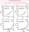 |
Fig. 1 Present calculated STS rates kturs compared to experiment and other calculations (in units of 10−20 m3 s−1). |
4 Discussion
As shown in Figs. 1 and 2, the present calculated STS rates match the available experimental values in the range 20 to 300 K very well. The STS rates from the Lee08 set are quite close to the present STS rates. Conversely, the STS rates from FR98 show some noticeable differences with respect to the present results, while the STS rates by Wan et al. (2018)1 are systematically lower than the present STS rates. These differences are far more evident in Fig. 3 where they are expressed asa percentage as
 (9)
(9)
where  are STS rates by other authors (oa), including the experimental ones, and
  are the STS rates calculated in the present work.
Figure 3 shows the good agreement between the present results and the experimental ones (dots) in the 20 to 300 K range in more detail, with differences between 5 and 10% for 20 ≤ T ≤ 50 K, and smaller than 5% for 50 ≤ T ≤ 300 K. The present STS rates depicted in Figs. 1 and 2 are the parametric polynomial description (in red, from 10 to 200 K) and the parametric Arrhenius-Kooij description (in green, from 100 to 1000 K) according to Eqs. (7) and (8), with the parameters from Tables 2 and 3, respectively. Other STS rates from Table 1 which are not depicted in Figs. 1–3 show similar degrees of accuracy compared to the experimental rates (Montero et al. 2020).
The FR98 set was calculated using the experimental energies of the rotational levels, which are very close to those of the present ![Mathematical equation: $[J(J+1)]^n$](/articles/aa/full_html/2021/03/aa39790-20/aa39790-20-eq15.png) , n ≤ 5, expansion. Thus, the large differences between the FR98 set and the present STS rates should be attributed to the different PESs employed and/or to other differences in the computational procedure.
, n ≤ 5, expansion. Thus, the large differences between the FR98 set and the present STS rates should be attributed to the different PESs employed and/or to other differences in the computational procedure.
On the other hand, Wan18 STS rates were calculated with the same P08-PES and MOLSCAT methodology of the present work. Hence, the systematic differences evident in Fig. 3 require some explanation. First, Wan18 rates were calculated using rigid rotor energies EJ = B0J(J + 1) with B0 = 60.853 cm−1 (Wan et al. 2018) while the present STS rates have been calculated with nearly exact rotational energies. We find that this difference in the rotational energies can lead to a substantial decrease in the STS rates (up to 30% for some transitions at low temperature). In addition, another computational detail deserves mention: calling the subroutine provided by Patkowski et al. (2008), the angle π − θb must be introduced as an argument instead of θb for consistency with the definitions used in the MOLSCAT code (Patkowski et al., priv. comm.). The combined effect of those computational differences might account, at least in part, for the differences found between Wan18 STS rates and the present ones.
The role of simultaneous excitation-de-excitation processes (up-down processes in short) also deserves mention. In these processes, one of the colliding partners gains energy while the other loses energy. The collision energy gap tends to be small, as can be seen in Table 1 for the 2543, 4123, and 0321 processes. Their gaps are about one-half smaller than the next single de-excitation processes, 2000 to 2505, where only one of the partners becomes de-excited while the other remains unchanged. As shown in Table 1, the STS rates of the up-down processes are considerably larger than those of the single de-excitation processes. Therefore, up-down processes do contribute significantly to the population-destruction equations (Black & van Dishoeck 1987; Sternberg & Dalgarno 1989) and cannot be ignored. Surprisingly, there are almost no reports about up-down STS rates in the literature with the exception of Monchick & Schaefer (1980) and previous works from our laboratory (Montero et al. 2006, 2020; Montero & Pérez-Ríos 2014). The quantitative importance of the 0321 up-down process was discussed in detail by Montero et al. (2020, Supp Material). Figures 1a and b show the relative values of k0321 and k4123 up-down rates compared to the dominant rates k3010, k3111 in Figs. 1c and d, and to k2000, k2101, k4020, and k4121 shown in Figs. 2a–d.
The statement by Flower & Roueff (1998) according to which the STS cross-sections for H2 :H2 inelastic collisions are insensitive to the rotational state of the perturber is not supported by the present results nor by the experiment (Montero et al. 2020). As shown in Table 1, the k2101 STS rate is considerably larger than k2000, namely 76% larger at 300 K, and 63% larger at 1000 K; k3111 is also largerthan k3010, that is, 26%larger at 300 K, and 40% larger at 1000 K. Those STS rates originate from the integration of the corresponding STS cross-sections according to Eq. (3), and hence the cross-sections are actually sensitive to the rotational state of the perturber. This happens at least for low values of the J rotational quantum number, those dominant in the 10 to 1000 K range.
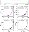 |
Fig. 2 Present calculated STS rates kturs compared to experiment and other calculations (in units of 10−20 m3 s−1). |
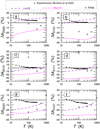 |
Fig. 3 Differences of experimental and other calculated STS rates with respect to the present calculation (Eq. (9)), in %. |
5 Conclusions
In this work the relevant STS rates for H2 :H2 inelastic collisions between 10 and 1000 K were calculated employing a recent version of the H2 -H2 PES and of the MOLSCAT code. Our main conclusions are
- 1.
The P08-PES (Patkowski et al. 2008) proves to be of very good quality in the range of energies involved in the STS rates compared with the experiment between 20 and 300 K (the relevant range of total energy being Etot ≤ 4500 cm−1) within the v = 0 vibrational state. Together with the recent version of the MOLSCAT code (Hutson & Le Sueur 2019), the P08-PES provides STS rates that are highly consistent with the experiment (Montero et al. 2020).
- 2.
The use of accurate experimental spectroscopic values for the energies of the rotational levels in v = 0 has substantially improved the accuracy of the STS rates calculated here.
- 3.
The pruned set of STS rates reported here is considered to be sufficiently complete for diagnostics between 10 and 1000 K based on the simulation of IR emission spectra combined with the population-destruction equations (Black & van Dishoeck 1987; Sternberg & Dalgarno 1989).
- 4.
The pruned set of STS rates reported here is expected to be substantial for the quantitative interpretation of gas dynamic processes involving H2, such as for instance, the experimental study of H2:H2O inelastic collisions.
The presentresults, especially the MR Tables, are hoped to be useful to the astrophysical community in the near future. The interpretation of a wealth of astronomical infrared spectroscopic data on H2 will probably benefit from the present results.
Acknowledgements
This work has been supported by the Spanish Ministerio de Economía y Competitividad (MINECO), grants FIS2017-84391-C2 and CONSOLIDER-ASTROMOL CSD2009-0038. We are indebted to K. Patkowski for the clarification about the use of the H2 +H2 potential energy surface subroutine. Thanks are due to P. C. Stancil for the h2.dat file with the STS rates corresponding to P08-PES calculation by Wan et al. (2018).
References
- Aguado, A., Suarez, C., & Paniagua, M. 1994, J. Chem. Phys., 101, 4004 [Google Scholar]
- Alexander, M. H., & Manolopoulos, D. E. 1987, J. Chem. Phys., 86, 2044 [NASA ADS] [CrossRef] [Google Scholar]
- Balakrishnan, N., Quemener, G., Forrey, R. C., Hinde, R. J., & Stancil, P. C. 2011, J. Chem. Phys., 134, 014301 [CrossRef] [PubMed] [Google Scholar]
- Black, J. H., & van Dishoeck, E. F. 1987, ApJ, 322, 412 [NASA ADS] [CrossRef] [Google Scholar]
- Boothroyd, A. I., Martin, P. G., Keogh, W. J., & Peterson, M. J. 2002, J. Chem. Phys., 116, 666 [CrossRef] [Google Scholar]
- Dalgarno, A. 2000, Molecular Hydrogen in Space (Cambridge Contemporary Astrophysics), eds. F. Combes, & G. Pineau des Forets (Cambridge: Cambridge University Press), 3 [Google Scholar]
- Diep, P., & Johnson, J. K. 2000, J. Chem. Phys., 112, 4465; 2000, 113, 3480 (erratum) [CrossRef] [Google Scholar]
- Dubernet, M. L., Alexander, M. H., Ba, Y. A., et al. 2013, A&A, 553, A50 [NASA ADS] [CrossRef] [EDP Sciences] [Google Scholar]
- Flower, D. R., & Roueff, E. 1998, J. Phys. B At. Mol. Opt. Phys., 31, 2935 [Google Scholar]
- Flower, D. R., & Roueff, E. 1999, J. Phys. B At. Mol. Opt. Phys., 32, 3399 [Google Scholar]
- Green. S 1975, J. Chem. Phys., 62, 2271 [NASA ADS] [CrossRef] [Google Scholar]
- Habart, E., Walmsley, M., Verstraete, L. et al. 2005, Space Sci. Rev., 119, 71 [Google Scholar]
- Hinde, R. J. 2008, J. Chem. Phys., 128, 154308 [CrossRef] [PubMed] [Google Scholar]
- Huestis, D. L. 2008, Planet Space Sci., 56, 1733 [Google Scholar]
- Hutson, J. M., & Le Sueur, C. R, 2019, Comp. Phys. Comm., 241, 9 [Google Scholar]
- Jennings, D. E., Weber, A., & Brault, J. W. 1987, J. Mol. Spectr., 126, 18 [Google Scholar]
- Lee, T.-G., Balakrishnan, N., Forrey, R. C., et al. 2008, ApJ, 689, 1105 [NASA ADS] [CrossRef] [Google Scholar]
- Lin, S. Y., & Guo, H. 2002, J. Chem. Phys., 117, 5183 [Google Scholar]
- Manolopoulos, D. E. 1986, J. Chem. Phys., 85, 6425 [NASA ADS] [CrossRef] [Google Scholar]
- Monchick, L., & Schaefer, J. 1980, J. Chem. Phys., 73, 6153 [NASA ADS] [CrossRef] [Google Scholar]
- Montero, S., & Pérez-Ríos, J. 2014, J. Chem. Phys., 141, 114301 [CrossRef] [PubMed] [Google Scholar]
- Montero, S., Thibault, F., Tejeda, G., & Fernández, J. M. 2006, J. Chem. Phys., 125, 124301 [Google Scholar]
- Montero, S., Tejeda, G., & Fernández, J. M. 2020, ApJS, 247, 14 [Google Scholar]
- Otto, F., Gatti, F., & Meyer, H. D. 2008, J. Chem. Phys., 128, 064305 [NASA ADS] [CrossRef] [Google Scholar]
- Patkowski, K., Cencek, W., Jankowski, P., et al. 2008, J. Chem. Phys., 129, 094304 [Google Scholar]
- Pérez-Ríos, J., Bartolomei, M., Campos-Martínez, J, Hernández, M. I., & Hernández-Lamoneda, R. 2009, J. Phys. Chem. A, 113, 14952 [Google Scholar]
- Pérez-Ríos, J., Tejeda, G., Fernández, J. M., Hernández, M. I., & Montero, S. 2011, J. Chem. Phys., 134, 174307 [Google Scholar]
- Roueff, E., Abgrall, H., Czachorowski, P., et al. 2019, A&A, 630, A58 [CrossRef] [EDP Sciences] [Google Scholar]
- Schwenke, D. W. 1988, J. Chem. Phys., 89, 2076 [NASA ADS] [CrossRef] [Google Scholar]
- Sternberg, A., & Dalgarno, A. 1989, ApJ, 338, 197 [NASA ADS] [CrossRef] [Google Scholar]
- Vissapragada, S., Buzard, C. F., Miller, K. A., et al. 2016, ApJ, 832, 31 [NASA ADS] [CrossRef] [Google Scholar]
- Wan, Y., Yang, B. H., Stancil, P. C., et al. 2018, ApJ, 862, 132 [Google Scholar]
Kindly reported by Stancil (priv. comm.) in h2.dat file.
All Tables
Calculated de-excitation STS rates for H2:H2 inelastic collisions in units of 10−20 m3 s−1.
Parametric description of de-excitation STS rates for H2:H2 inelastic collisions between 10 and 200 K.
Parametric description of de-excitation STS rates for H2:H2 inelastic collisions between 100 and 1000 K.
All Figures
|
Fig. 1 Present calculated STS rates kturs compared to experiment and other calculations (in units of 10−20 m3 s−1). |
| In the text | |
|
Fig. 2 Present calculated STS rates kturs compared to experiment and other calculations (in units of 10−20 m3 s−1). |
| In the text | |
|
Fig. 3 Differences of experimental and other calculated STS rates with respect to the present calculation (Eq. (9)), in %. |
| In the text | |
Current usage metrics show cumulative count of Article Views (full-text article views including HTML views, PDF and ePub downloads, according to the available data) and Abstracts Views on Vision4Press platform.
Data correspond to usage on the plateform after 2015. The current usage metrics is available 48-96 hours after online publication and is updated daily on week days.
Initial download of the metrics may take a while.