| Issue |
A&A
Volume 646, February 2021
|
|
|---|---|---|
| Article Number | A136 | |
| Number of page(s) | 13 | |
| Section | Planets and planetary systems | |
| DOI | https://doi.org/10.1051/0004-6361/202039050 | |
| Published online | 19 February 2021 | |
Revealing peculiar exoplanetary shadows from transit light curves
1
Space Research Institute (IWF), Austrian Academy of Sciences,
Schmiedlstrasse 6,
8042
Graz, Austria
e-mail: oleksiy.arkhypov@oeaw.ac.at
2
Institute of Astronomy of the Russian Academy of Sciences,
119017
Moscow,
Russia
e-mail: maxim.khodachenko@oeaw.ac.at
3
Institute of Laser Physics, SB RAS,
Novosibirsk
630090, Russia
4
Institute of Physics, Karl-Franzens University of Graz,
Universitätsplatz 5,
8010
Graz, Austria
e-mail: arnold.hanslmeier@uni-graz.at
Received:
28
July
2020
Accepted:
4
December
2020
Context. Until now the search of peculiar exoplanetary shadows, particularly those caused by exorings, was focused on the detection of a second-order photometric difference between the ringed and ringless (circular) transiting shadows. Both scenarios involved the parameter fitting to approximate the corresponding transit light curves (TLCs). As a result, the searched difference was extremely difficult to detect in the noise of the real transit photometry signals.
Aims. In this work, we look for photometric manifestations of a non-spherical obscuring matter (e.g., exorings) around different exoplanets, mainly hot Jupiters, using a principally new approach.
Methods. We used the transit parameters provided in Kepler database from the NASA Exoplanet Archive, where the fitting of the TLCs gives consistent sets of parameters for the transiting objects, assuming their spherical shape. At the same time, the semimajor axes, expressed in units of the stellar radii (initially, also a subject of the fitting), finally appear to be replaced by the calculated values according the Kepler’s third law and known stellar radii and surface gravity that have been determined through other methods. In the most typical case of a spherical transiting planet, such a replacement does not break the consistency of the whole parameter set. However, in the case of a non-spherical transiter and its non-circular shadow, the real (i.e., calculated according physics) value of the orbital semimajor axis could become inconsistent with the rest of the transit parameter set defined with the standard fitting procedure. The search for such inconsistencies, manifested as the difference between the simulated and observed transit duration, constitutes one of the main goals of this work. Moreover, we elaborate on a particular technique to gain information about the shape of planetary shadow, using the derivatives of the TLC during the ingress and egress phases.
Results. We checked the TLCs of 21 hot Jupiters and 2 hot Neptunes. The consistent transit parameters and quasi-circular shadows were found for 11 objects. The analysis of the TLCs of five of the objects is complicated due to the noise problems, leading to the instability of solutions and deformation of shadows due to the low resolution of the derivatives. The remaining seven objects were formally qualified as peculiar outliers and among them, the planets Kepler-45b and Kepler-840b appear to be the most intriguing targets, with the most significant inconsistency of the parameter sets and the shadows elongated along their orbital path.
Conclusions. We propose a new method for probing of planetary shape that confirms the circular transiting shadows for the majority of objects on the considered list. However, several objects exhibiting peculiar shadows have been discovered. These finds could be interpreted in terms of planetary dusty envelopes or exorings. The obtained results and elaborated methodology are relevant in the context of today’s photometry space missions, such as TESS, CHEOPS, and others.
Key words: planets and satellites: general / planets and satellites: detection / zodiacal dust
© ESO 2021
1 Introduction
Traditionally, the shape of a transiting exoplanet is a priori supposed to be that of a naked sphere (Li et al. 2019, and therein). However, matter rings around exoplanets (thereafter, exorings) (Heising et al. 2015; Aizawa et al. 2017), as well as oblateness (Biersteker & Schlichting 2017) and near-planet dust clouds (Arkhypov et al. 2019) would distort the circular planetary silhouette. At the same time, the general deduction of an image of shadow of a transiting object from its stellar light curve, without postulating of a particular physical model, encounters difficulties when dealing with degeneracies, low resolution, processing artifacts, and the selectivity aspect with regard to the geometry and analysis algorithms (Sandford & Kipping 2019).
While intensive searches for exorings were previously undertaken in Kepler’s photometry (Heising et al. 2015; Aizawa et al. 2017, 2018), these gave either negative or probabilistically hypothetic results. A notable exception has appeared in the system of the giant circumplanetary rings of J1407b (e.g., Kenworthy & Mamajek 2015). Their inferred radius of ~1 au implies that these rings are a rather exotic case. In fact, the detection of exorings remains one of the most appealing, albeit demonstrably challenging, goals in the field of exoplanetary science.
In this work, we propose and elaborate on a special method for the detection and probing of possible non-spherical shapes of exoplanetary silhouettes. Our method is explained in Sect. 2. The obtained results are described in Sect. 3 and we present our conclusions in Sect. 4.
2 Analysis method
Previous searches for exorings in Kepler data (Heising et al. 2015; Aizawa et al. 2017, 2018) yielded no convincing candidate findings. This fact leads to attempts to develop more sensitive methods. Here, we try one possible method for the detection and diagnostics of non-circular transiting shadows.
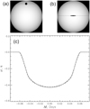 |
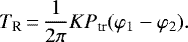
Fig. 1 Example of TLC proximity for different transit geometries. Panel a: model of a spherical object with β = 0.796 and ap = 0.032 au; panel b: model of an elongated disk-type shape of the transiting shadow (a thin disk with an increased radius of 2.59 times of that in the case of mode (a) and tilt of 6.38 deg.), keeping the same depth of TLC minimum, with β = 0.054 and ap = 0.053 au; panelc: combination of synthetic TLCs calculated for the models (a) (dashed line) and (b) (solid line). The orbital period and stellar parameters are the same in both models. Here, ΔF is the decrease of the radiation flux caused by the transiting object. The abscissa parameter Δt is the time relative to the predicted transit mid-time. |
2.1 Limitations of previous studies
Hitherto, the standard method for searches of exoring signatures in Kepler data (Heising et al. 2015; Aizawa et al. 2017, 2018; Akinsanmi et al. 2020)consisted of using of a phase-folded transit light curve (TLC) to fit the parameters of an exoplanet, that is, the planetary radius, Rp, impact parameter, β, semi-major orbital axis, ap, the radii of ring borders, the ring transparency and its positional angle. These values were considered as free parameters to be fitted for two models: (a) the case of a ringless spherical planet; and (b) the ringed (or disk-carrying) body. Using these fitted parameters, the synthetic light curves were calculated for both models and compared with the real TLC. The ring detection was assumed in the case of a significantly better approximation of the observed TLC by the model (b), as compared to the ringless model (a).
However, in practice, both models (a) and (b) can generate very similar TLCs. For example, Fig. 1 shows the proximity of two synthetic TLCs, calculated (see details in Appendix A) for the cases of a spherical and disk-type models of the transiting object, with different values of β and ap attributed to them, but using the same (i.e., fixed) transit (or orbital) period Ptr, transiter’s cross-section (i.e., total obscuring area) and stellar parameters. In the considered example, the increase of the transiter’s size along the direction of its orbital motion, in the case of a disk-type object, can be compensated by a longer trajectory across the stellar disk to keep the TLC shape practically unchanged. The corresponding impact parameter, therefore, should be decreased from β = 0.796 in the case of a spherical transiter (model (a)) down to β = 0.053 for the disk-type object (model (b)). At the same time, in order to keep the transit duration unchanged, the linear velocity, ∝ ap∕Ptr, of the transiter, crossing the stellar disk along the longer trajectory, should be higher. Since the orbital period is rigidly determined by the observed transit periodicity Ptr, the increaseof linear velocity in the case of a disk-type object requies an increase of ap = 0.053, instead of 0.032 au.
This example demonstrates how the simple fitting of the orbital parameters, ap and β, could emulate the ring-effect in the case of a spherical transiting object. Since all the previous studies were based on the fitting to the simple ringless model as a reference standard, the search for exorings, in fact, consisted of focusing on the tiny second-order effects, hidden in the noisy TLCs. Such an approach decreased the survey sensitivity, limiting the chances of a real ring detection.
Zuluaga et al. (2015) proposed framing the search for exoring manifestation in the form of significant increase in the transit depth that might lead to a misclassification of the ringed planetary candidates as false-positives or underestimations of the planetary density. However, the traditional interpretation of such effects as stellar eclipses and planetary super-puffs, makes the proposed approach only a hypothetical one. Another idea considered in Zuluaga et al. (2015) concerns the search of discrepancies between the stellar density values found from TLCs and those revealed through other independent methods, such as stellar models, asteroseismology, or transits of other planetary companions. Unfortunately, this interesting approach is elaborated upon using a simplified model, ignoring the limb-darkening over stellar disk. Moreover, anomalous cases revealed in the predeceasing study by Sliski & Kipping (2014) were interpreted in terms of non-zero eccentricities of the planetary orbits and confusion of the stars’ identification. Although some such finds could be manifestations of exorings, no other surveys were implemented to check this according to the propositions by Zuluaga et al. (2015). In any case, the approach in Zuluaga et al. (2015) is focused on spotting excessive matter around the transiting object (exorings) and related density anomalies, so it would not be efficient in case of a planet with a normal density, but with a non-spherical shape. In general, the density-based methods require precise measurements of planetary and stellar masses and sizes and, thus, this requirement limits their applicability.
2.2 Key ideas for the new approach
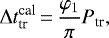
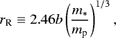
We call attention to the fact that in the NASA Exoplanet Archive1 (hereafter, NASA EA), the ratio of orbital semi-major axis, ap and stellar radius, R*, is not a free parameter, as it should be, according to the formal TLC fitting procedure applied there. Instead of being determined from the fitted ratio ap∕R*, the value of ap, given in the NASA EA, is derived fromthe transit period, Ptr, which is equal to the orbital period, defined by the Kepler’s third law (Li et al. 2019) as follows:
 (1)
(1)
where g is the acceleration due to gravity in the photosphere of the planet hosting star. The related stellar parameter log (g), needed for specifying g in Eq. (1), is measured separately (Mathur et al. 2017), whereas the stellar radius, R*, which is also included in the NASA EA, is taken from the revised Kepler Input Catalog, where it was fitted using the photometricdata and stellar models (Huber et al. 2014). Therefore, the fixed and independently defined values of ap and R* in the NASA EA exclude the above-shown confusion between two possible shapes of the transiting shadow as illustrated in Fig. 1.
Thus, it seems reasonable to use the data (ap, Rp, β, R*) from the NASA EA instead of their simple re-fitting. However, this data set is self-consistent only in the case of a circular shadow of the transiter, whereas for the non-spherical transiting object, this is not so. In fact, in the case of a spherical body, the observed ingress or egress time would be consistent with the prediction based on the parameters from NASA EA, which were fitted using the spherical model of transiting object, even in spite of the fact of further substitution of the fitted ap ∕R* with the independently measured parameters. However, in the case of a non-spherical object, the values ap and R* in the NASA EA, still defined from the celestial mechanics and independent measurements, will not be consistent with the rest of the fitted parameter set since the latter would have another value of ap ∕R*. Altogether, this will result in a difference between the reconstructed TLC based on the parameters from the NASA EA and its accurately measured analog. Therefore, any significant discrepancy between the transiter’s model prediction based on the parameters from the NASA EA and the real ingress or egress timing in the measured TLC could indicate about an elongated transiting shadow. This effect enables the possibility of searching the ringed planets using the timescale of TLC slopes as a first-order manifestation of the transiting object’s shape.
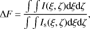
To demonstrate the key idea behind our method, let us consider as the transit background, a simplified case of a homogeneous stellar disc with the constant brightness  , corresponding to the integral radiation flux, Fb. The transiting exoplanet distorts the stellar flux, resulting in F(t), where t is time. For the analysis, we introduce the time difference, τ = t − t0 in the ingress and τ = t0 − t in the egress parts of a TLC, respectively, where t0 is the start time of the planetary ingress or the end time of its egress. Correspondingly, the ingress (or egress) part of the TLC at a certain moment, τ = τ*, could be considered as the sum
  of the contributions − Bs(τi)Δτi of flux absorption produced by the elementary areas, consequentially added to the growing (or decreasing) planetary shadow with each (sufficiently short) time step Δτi. Every such elementary area has the size s(τi)Δτi, where s(τi) is the speed ofarea change from one time step to another. In fact, the above discrete summation process at the limit of Δτi → 0 corresponds the integral
 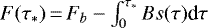 .
.
By taking derivative of the above integral expression for F(τ*), we can obtain |∂F∕∂τ*| = Bs(τ*) ≡|∂F∕∂t|. This means that the derivative |∂F∕∂t| at a given time moment τ = τ* is ∝ s(τ*). Hence, it reflects the 1D-distribution of the obscuring matter. The maximum value of |∂F∕∂t| corresponds to the moment when the thickest part of the transiter’s shadow crosses the stellar limb. Altogether, by transforming the time into space coordinate, we could test the hypothesis regarding a circular shape of the transiting object’s shadow, passing across the stellar disk. However, for the correctness of the treatment, the stellar limb-darkening must be taken into account as a distorting factor that affects the brightness, B.
2.3 Methodological basis
We use the public Kepler TLCs from NASA EA in short cadences after the implemented Pre-search Data Conditioning. With an iterative exclusion of outliers and further whitening (for details, see Arkhypov et al. 2019, 2020), we prepare for each investigated transiting object, a phase-folded TLC, as shown for example in Fig. 2a, which represents the decrease of flux, ΔF(Δt), during the transit, to be analyzed further. A consideration of the phase-folded TLCs enables us to increase of precision of the analysis and, specifically, the accuracy of defining the TLC derivative in the ingress and egress parts. Here, Δt is the time counted from the nearest transit mid-time, calculated for each transit using the available cumulative transit elements (i.e., reference time, period, and duration) from the NASA EA. Our method is based on the analysis of the temporal behavior of the derivative D ≡ ∂(ΔF)∕∂(Δt) during the ingress and egress phases (Fig. 2b). As argued in Sect. 2.2, it enables an approximate sensing of the 1D spatial distribution of the transiting obscuring matter. We use a certain part of the derivative curve, marked in red in Fig. 2b, which is the most sensitive to the shape of transiting object. It is worth to noting that the derivatives of the ingress and egress parts of a TLC are also minimally affected by starspots, as their contribution is projectively reduced near the stellar limb.
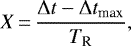
The main task consists of carrying out the conversion of Δt and D to the dimensionless coordinates X and Y (normalized to the planetary catalogue radius Rp) in the orthogonal coordinate system, co-centered with the transiter’s shadow, as shown in Fig. 3. Taking X-axis pointed from the shadow’s center to the center of stellar disc for the egress, and oppositely for the ingress phases, we can write:
 (2)
(2)
 (3)
(3)
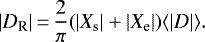
where Δtmax is the time of maximal |D|, estimated separately for the ingress and egress parts of the TLC; TR is the time which corresponds the ingress/egress of the planetary radius Rp, and |DR | is an absolute value of the derivative achieved at this time. Thus, a spherical planet has a circular shadow with a normalized radius of 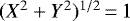 and an area π. In order to preserve the observed flux decrease in the TLC during the transit, the shadow area has to be the same also for any other transiter’s shape, so that π = 2(|Xs| + |Xe|)⟨|Y |⟩. Here, |Xs| and |Xe | are the maximal absolute values of X at the observed start, Δtstart, and end, Δtend, times of the transit, respectively; ⟨Y ⟩ = ⟨|D|⟩∕|DR|, where ⟨|D|⟩ is the averaged over Δtstart < Δt < Δtmax (for the ingress) and Δtmax < Δt < Δtend (for the egress) absolute derivative |D|. Therefore, using Eq. (3), we can obtain
 (4)
(4)
The timescale, TR, can be found for a circular shadow using the transit cumulative data from NASA EA:
 (5)
(5)
Here, φ1 = arctan(ΔX1∕r) and φ2 = arctan(ΔX2∕r), where ![$\Delta X_{1}\,{=}\,[(R_{*}+R_{\textrm{p}})^{2}-(\beta R_{*})^{2}]^{1/2}$](/articles/aa/full_html/2021/02/aa39050-20/aa39050-20-eq10.png) ,
, ![$\Delta X_{2}\,{=}\,[R_{*}^{2}-(\beta R_{*})^{2}]^{1/2}$](/articles/aa/full_html/2021/02/aa39050-20/aa39050-20-eq11.png) ,
, ![$r\,{=}\,[a_{\textrm{p}}^{2}-(\beta R_{*})^{2}]^{1/2}$](/articles/aa/full_html/2021/02/aa39050-20/aa39050-20-eq12.png) , and Ptr is the period of transit. To correct the slight shift of Δtmax due to limb-darkening, the factor K = (|Xs| + |Xe|)∕2, which in the considered further set of objects stays between 1.12 and 1.31, is applied in Eq. (5). This factor is calculated using the synthetic TLC prepared for a spherical transiting exoplanet and the best limb-darkening approximation from Claret & Bloemen (2011) for the given system parameters from NASA EA. Since the integral photometry cannot distinguish between Y and − Y, both options are considered in the course of the silhouette reconstruction.
, and Ptr is the period of transit. To correct the slight shift of Δtmax due to limb-darkening, the factor K = (|Xs| + |Xe|)∕2, which in the considered further set of objects stays between 1.12 and 1.31, is applied in Eq. (5). This factor is calculated using the synthetic TLC prepared for a spherical transiting exoplanet and the best limb-darkening approximation from Claret & Bloemen (2011) for the given system parameters from NASA EA. Since the integral photometry cannot distinguish between Y and − Y, both options are considered in the course of the silhouette reconstruction.
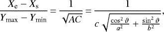
The proposed methodology for the reconstruction of possibly non-circular silhouettes of the transiting objects works correctly only for the Y -symmetric shadows and in the case of sufficiently small impact factors, β. In spite of this, it can be still used for any β as an indicator of the transiters’ shape anomalies and complexity (e.g., oblateness, exoring, circumplanetary disc with forming satellites, etc.). We note that for the spherical transiters, the method equally works for any value of β (excluding the cases of degenerated grazing transits with the partial eclipse).
For the demonstration of method capabilities and limitations, we consider the case of confirmed exoplanet Kepler-1b orbiting the star KIC 11446443 with the high impact parameter β = 0.818. Figure 4 shows a quasi-circular exoplanetary disc reconstructed from the synthetic TLC. The ratio of sizes of the resulting contour along the coordinate axes X and Y is predictably close to unity (Xe − Xs)∕(Ymax − Ymin) = 1.03 ± 0.04. Here Ymax, Ymin are the extremal estimates of Y. Since the transiter’s sizes Xe − Xs and Ymax − Ymin are related via Eq. (4), we can characterize the transiter’s shape using only one value (Xe− Xs)∕2 = 1.01 ± 0.05, which is defined in units of radius Rp of the equivalent spherical transiting object.
At the same time, this value significantly differs from unit in the cases simulated in Figs. 5 and 6. For the simulation with a ring in Fig. 5 (see Appendix A for details), it is 1.41 ± 0.07. The reconstructed silhouette (bottom panel in Fig. 5), in general, resembles the input geometry of the transiting object (upper panel in Fig. 5) but with some distortions caused by the case geometry effects related to the treatment of the inclined stellar limb. Figure 6 shows one more model, in which the planet is surrounded by an absorbing halo of the tripled radius and transparency 95% and orbits the same star KIC 11446443, as in Figs. 4 and 5. The planetary radius is slightly decreased in order to conserve the total effective obscuring area of the transiting object. Such models with a halo may be of interest with respect of the numerical simulations of a disturbed exoring in Sucerquia et al. (2017). In the reconstructed silhouette of the transiter in Fig. 6, an abnormal elongation of shadow along the Y -axis is clearly seen.Altogether, the silhouettes, like those in Figs. 5 and 6, can be considered as possible indicators ofpeculiarity of the shape of transiting objects.
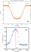 |
Fig. 2 Example of a KOI 1.01. Panel a: folded TLC; panel b: derivatives of the TLC’s ingress (squares) and egress (crosses) parts. The analyzed part of the derivative is marked in red. |
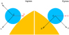 |
Fig. 3 Moving, co-centered with planet, orthogonal coordinate system (X, Y), used for the calculation of D. The planetary disc (blue circle), with the center of coordinate “C”, obscures the stellar disk (yellow segment), moving across it with the projected velocity V (red vector). The X-axis is pointed to the center of stellar disc, for the egress (right panel), and opposite, for the ingress (left panel) phases, respectively. |
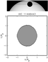 |
Fig. 4 Trial reconstruction of transiter’s silhouette (bottom panel) of Kepler-1b at KIC 11446443, using the synthetic TLC simulated for a spherical transiter with the radius and transit geometry of the planet taken from NASA EA. Vertical bars in the restored silhouette depict its uncertainty (± standard error). The simulated transit geometry, used for the calculation of K-factor in Eq. (5), is illustrated in upper panel. The horizontal solid line shows the trajectory of transiter across the stellar disk. |
2.4 Maintechnical details
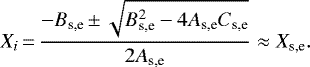
The real radius of transiting object could be found as, for example, Xe or Xs, to compare with the fitted value of Rp from NASA EA. Such an estimation depends critically on the localization of the border and the maximum of the TLC’s derivative, ∂(ΔF)∕∂(Δt) ≡ D. The derivative values, Dj in the jth time moments Δtj are found by mean squares method giving the regression, F(Δt) = DjΔt + Cj, which approximates the TLC parts in adjoining equidistant time-intervals jδt < Δt < (j + 1)δt. Here, Cj is the fitted constant, and δt is the time resolution of the derivative. This resolution is iteratively fitted to ensure the accuracy of at least 10% for the best estimating |Dj |. We determine the derivative value |Dj|, its standard error, σD, and the corresponding averaged time, Δtj = ⟨Δt⟩, for each time interval, ± δt, around Δtj, as shown in Fig. 2b. The values of Δtj as well as of Δtj*≡ Δtmax at the j*th moment when |Dj |≡|Dj*| achieves its maximum, that is, |Dj*| = max(|Dj|), are substituted in Eq. (2) to obtain the corresponding Xj.
Using the obtained values of Δtj and |Dj|, we can localize the borders, |Xs| and |Xe|, of the ingress and egress derivatives, respectively, needed for Eq. (4), which also correspond to the start and end of the transit. This procedure is realized in the following approximation steps:
First, we select the derivative estimates with |Dj| > 0.5max(|Dj|) = 0.5|Dj*| from the search interval, |Δtmax|− TR < |Δtj| < 0.5Δttr + 0.05 days, where Δttr stays for the duration of transit, taken from NASA EA, and the value of 0.05 days is an empirically defined search margin. This margin was selected empirically after several iterating processing trials. In practice, there is no noticeable systematic influence of this value on the analysis results. The obtained selection is approximated by quadratic polynomial. Its maximal root, Δtlim, gives a rough (in fact, overestimated) absolute value of the derivative border. The polynomial maximum localizes the maximum of the derivative |Dmax| at the time |Δtmax2| more accurately.
Then a more precise selection of the derivative’s points is carried out in the interval, |Δtmax2| < |Δtj| < Δtlim, using the condition |Dj| > 2σb. Here σb is a standard deviation of the transit background at |Δtj| > |Δtmax| + TR. Thereafter, we can substitute the selected |Δtj| and |Δtmax2| instead of Δtmax and Δt in Eq. (2) to obtain the corresponding Xj. The boundaries of interval Xs = − max(|Xj|) and Xe = max(|Xj|), at which the derivatives are searched, are found separately using the corresponding data sets for the ingress and egress, respectively.
The obtained values of Xs and Xe are then substituted in Eq. (4), as well as the parameter ⟨|Dj|⟩, which is averaged over the both ingress and egress data to minimize a function gap at X = 0. The found scale, |DR |, is used in Eq. (3) to calculate the ordinate value, Yj, for the contour of transiting object. The error of Yj is estimated as:
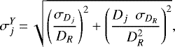 (6)
(6)
where  is the standard error of DR:
![\begin{equation*} \sigma_{D_{R}}\,{=}\,\sqrt{\left [ \frac{2}{\pi} (X_{e}-X_{s})\sigma_{\langle |D| \rangle} \right ]^{2} + \left (\langle |D| \rangle \right. \sigma_{X})^{2} + \left (\sigma_{X} \sigma_{\langle |D| \rangle} \right)^{2}},\end{equation*}](/articles/aa/full_html/2021/02/aa39050-20/aa39050-20-eq15.png) (7)
(7)
where: σX is the standard error of estimating Xe − Xs due to the limited resolution of Dj, and σ⟨|D|⟩ is the standard error of ⟨|D|⟩.
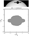 |
Fig. 5 Model of transiting object with a ring (upper panel), built on the basis of the real object KIC11446443, to simulate TLC of a ringed planet. The total area of obscuration is the same as in Fig. 4. The reconstructed silhouette (bottom panel), obtained from the synthetic TLC reveals the presence of the distorting structure. |
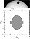 |
Fig. 6 Transiter model with a halo (upper panel), built on the basis of real object KIC11446443. The total area of obscuration is the same as in Fig. 4. The reconstructed silhouette (bottom panel), obtained from the synthetic TLC reveals the distortion of the circular shape of planetary shadow. |
2.5 Application aspects
We consider the published cumulative values of ap, β, R*, Rp and Ptr from the NASA EA as a given set of model constants and ignore their errors. The first goal of our study is to determine the degree of self-consistency of this set using the parameter 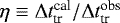 . Here, the observed transit duration,
  , is also adopted from the NASA EA (see the KOI cumulative list) and
  is calculated using the whole aforementioned set of published parameters from the same source:
 (8)
(8)
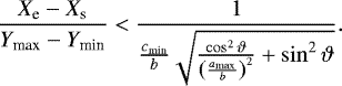
where φ1 has been specified above with respect of Eq. (5)). When the parameter  appears to be clearly different from the unit, it indicates a possible peculiarity (i.e., a non-circular shape) of the transiter’s shadow.
The additional indicators of shadow’s peculiarity are the values |Xs | and |Xe |, in other words, the empirical half-diameter of the shadow, expressed via the planetary radius, taken from NASA EA. If the inconsistency of the transit parameters is controlled only by the orbit radius, ap, there is a simple relation between |Xs,e| and  . Since the values of ΔX1,2∕r, specified in the definition of Eq. (5) are small parameters, we can approximate φ1,2 ≈ ΔX1,2∕r. Therefore, for
  , the approximation r ≈ ap in Eq. (5) leads to the proportionality TR ∝ 1∕ap. Substituting this result in Eq. (2), we obtain |Xs,e|∝ ap. In accordance with Eq. (8), another relation takes place, namely,
  . Hence, |Xs,e| = Q∕η, where Q is a constant. Since both, |Xs,e| = 1 and η = 1 for a consistent parameter set, we can obtain Q = 1. Hence, the desired relation is:
 (9)
(9)
The deviation from Eq. (9) (we note that this equation is valid for the case of spherical transiting objects) could indicate non-circular shadows even in the quasi-self-consistent cases with 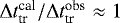 .
.
A suspected non-circular shadow can be visualized and studied using the above method of the transformation of the TLC derivative into XY-diagram, as in Fig. 4. To formalize this procedure, we approximate the obtained points of the shadow contour with the i-numbered coordinates, Xi and Yi, by the quadratic polynomial
 (10)
(10)
where As,e, Bs,e and Cs,e are the coefficients fitted separately for ingress and egress data sets (“s” and “e” indexes, respectively). In fact, this second-order polynomial corresponds to an ellipse segment. For a circular shadow, the condition Bs,e = 0 is obvious. It is important to remember that variation of ap leads to the variation of orbital velocity, which for the given measured TLC, would result, according to Eq. (2), in the elongation or shrinking of the shadow along the coordinate axis X without any generation of non-zero Bs,e. Hence, the condition that Bs,e≠0 is another indicator of the shadow’s peculiarity, which is independent from the variation of ap.
For Xi = 0, the condition 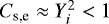 means the compression of planetary shadow along Y -axis and the corresponding elongation in the direction of X since the total area of shadow is a constant value, keeping the depth of the TLC minimum unchanged. Correspondingly, we find for Yi = 0 :
 (11)
(11)
If |Xs,e| > 1, then the maximal |Yi| has to be <1 at Xi = 0. Such an elongation in the X direction could correspond to an opaque circumplanetary disk or exorings that are slightly inclined relative the orbital plane. In contrast, the shadows with Cs,e > 1, and correspondingly Xs,e < 1, may indicate the presence of weakly absorbing dust around the planet. Such dust may detectably increase the effective area of the transiting shadow and the related estimate of Rp in NASA EA, while the derivative reveals the true planetary radius Xs,e < 1 in the units of the officially published Rp.
3 Survey of non-spherical transiting object cases
3.1 Compilation of the dataset
The dataset considered here is comprised of 23 Kepler objects of interest (KOIs). The results obtained for these objects are presented in Table 1. Our targets were selected among the best observed objects from the list by Aizawa et al. (2018) which do not have a current status of “false positive” in the NASA EA. To avoid inter-transitinterference in multi-planetary systems, only the cases with a single transiting object were included in our data set. We have effectively exhausted all Kepler data suitable for the qualitative analysis of the derivatives ∂(ΔF)∕∂(Δt).
The highest status mark, “p!”, is assigned in Table 1 to the confirmed exoplanets with measured masses below 13 MJ (here, MJ is the mass of Jupiter). In fact, 78% of all objects in the considered data set belong to this group. Four confirmed planets with unknown masses are marked with “p” (17% of objects), whereas one unconfirmed candidate (KOI 883.01) is given the status index “c” (4% of objects). We assign to the object KOI 1416.01 in Table 1, the status of “p?” because it is currently classified in the Kepler data catalogue of NASA EA as a false positive, but at the same time, it is included on the list of confirmed objects of the same catalog. Another case – KOI 194.01 – has in our data set an interrogative status “p?” due to its previous, but probably obsolete, classification as a false positive in the Kepler data catalogue, whereas in NASA EA, this object is marked as confirmed. The asterisk extension of the assigned status indexes in Table 1 marks objects, which have the status of confirmed planets with the measured planetary masses, while being still given the stellar eclipse flag in the Kepler data catalogue, such as KOI 13.01, KOI 18.01, and KOI 202.01.
There isa special notation in the KOI Cumulative List of NASA EA for KOIs “that are observed to have a significant secondary event” [i.e., the secondary TLC minimum due to the eclipse of the planet by the star], “transit shape or out-of-eclipse variability” indicating that the transit-like event is most likely caused by an eclipsing binary. “However, self-luminous, hot Jupiters with a visible secondary eclipse will also have this flag set, but with a disposition of PC” [i.e., a planetary candidate].
For example, the objects KOI 13.01 and KOI 18.01 (Kepler-13b and Kepler-5b), orbiting the stars KIC 9941662 and KIC 8191672, respectively, which are included in our set, have the stellar eclipse false positive flag in the KOI Cumulative List of NASA EA. Nevertheless, the measurements of their masses by two different methods give us the non-stellar values (Esteves et al. 2013) corresponding to the classification of objects as confirmed planets in the same NASA EA. As for the observed secondary eclipses, they are an important instrument of exoplanet meteorology that are used in many dedicated studies of genuine hot Jupiters (e.g., Jackson et al. 2019; Pass et al. 2019).
Figure 7 shows the distribution of transiting KOIs in our analyzed targets data set over their radii, Rp, and orbital semimajor axes, ap, as given in NASA EA. As it can be seen, the target list includes mainly hot jupiters with an admixture (9%) of hot neptunes (KOI 3.01 and KOI 63.01).
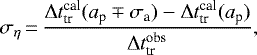
Table 1 shows the local radii |Xs| and |Xe| of every transiting shadow at the first and last contacts, respectively. Their given errors are determined by the duration of time interval δt which includes the TLC points, used to calculate one point of the derivative, D (i.e., Dj at jth time moment, Δtj, as described in Sect. 2.4). Due to such a discretisation, the true border of the derivative can be different from the accepted value |Xs,e|, with an uncertainty of up to σx = ± 0.5δt∕TR, which is also given in Table 1.
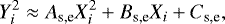
Another characteristic value in Table 1 is the ratio,  , which indicates the degree of consistency of the transit parameter set. As discussed in Sect. 2.2, this consistency can be distorted by the actual use of physically estimated orbital radius ap (see Eq. (1)), instead of the fitted value, which together with other fitted parameters provides the best approximation of the measured TLC.
The standard error σa of the applied ap can be calculated as follows:
![\begin{equation*} \sigma_{\textrm{a}}\,{=}\,{\pm}\sqrt{[a_{\textrm{p}}(z\,{\pm}\,\sigma_{z})-a_{\textrm{p}}(z)]^2 + [a_{\textrm{p}}(R_{*}\,{\pm}\,\sigma_{R*})-a_{\textrm{p}}(R_{*})]^2},\end{equation*}](/articles/aa/full_html/2021/02/aa39050-20/aa39050-20-eq30.png) (12)
(12)
where ap, as a function of arguments z ≡ log(g) and R*, is defined by Eq. (1), assuming the corresponding errors ± σz and ± σR* in definition of z and R*, respectively. Other parameters are considered as constants, provided in the NASA EA. The values for z ≡ log(g) and σz, as well as for R* and σR* are taken from the KOI Cumulative List in the NASA EA. Therefore, in a similar way, we can find the error, ση, of the ratio η:
 (13)
(13)
where  is defined by Eq. (8) with the varying argument ap, whereas other arguments (R*, Rp, β and Ptr) are considered here as constants provided in the NASA EA. The calculated so upper and lower values of the error ση are listed in Table 1 (in the η-column).
Analyzed target set and the main processing results.
3.2 Phenomenology of transit shadows
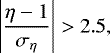
Figure 8 shows the found values (listed also in Table 1) of the parameter consistency indexes |Xs,e| and η. These values are ingeneral consistent with the predicted relationship Eq. (9), which confirms the above assumption on the leading role of ap in the mismatch of the parameter set. There also exist a major cluster of presumably normal (quasi-circular) shadows with |Xs,e|≈ 1 and 0.95≲ η ≲ 1.2. This cluster can be formally defined by an iterative process aimed at progressive exclusion of outliers, using the criterion |η −⟨η⟩| > 2.5σ, where 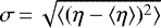 is the current standard deviation of η from its mean value ⟨η⟩ in the cluster. This iterative process is stopped when the value σ becomes invariable from one step to another. As an outcome of such procedure, it was found that about 87% (i.e., 20 objects) are clustering around the center at ⟨|Xs,e|⟩ = 0.99 ± 0.02 and ⟨η⟩ = 1.06 ± 0.01. The proximity to unit of ⟨|Xs,e|⟩ and ⟨η⟩ means the statistical accordance between the fitted and independently measured transit parameters; in other words, their consistency in majority of the cases, which, in turn, confirms the validity of an a priori assumption, in these cases, of the spherical shape of the transiter.
Since the transit parameters were fitted for the standard a priori assumed model of the spherical shape of a transiting object (i.e., planet), we can expect the circular shadows in XY -diagrams, as in Fig. 4. Figure 9 shows the examples of such circular shadows reconstructed for the objects from the above mentioned central cluster in Fig. 8.
The case of η≠1 manifests an inconsistency in the form of elongated shadows in XY -diagrams, as those in Fig. 10. For example, the planet Kepler-45b orbiting KIC 5794240 shows clear elongation (Fig. 10a) reflecting the slightly inconsistent transit parameter set of 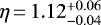 . Another planet Kepler-840b orbiting KIC 11517719 has an obviously inconsistent value of
 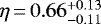 and a well-defined elliptical shadow in Fig. 10b.
The planet Kepler-670b orbiting KIC 11414511 has practically consistent value of 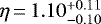 , but noticeable elongation in the direction of Y (Fig. 10c). This effect is a typical manifestation of noise in the derivative D, when the necessary derivative accuracy (≤10%) is achieved by the decreasing of the time resolution. As a result, the planetary border |Xs,e| (i.e., the start or end of transit) could be underestimated, which automatically results in overestimated values for Y, appeared to keep the TLC depth unchanged (see Eqs. (3) and (4)).
Another Y -elongated planet Kepler-13b orbiting the star KIC 9941662 (Fig. 11d) has an overly uncertain value of 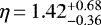 . However, a formally acceptable correction, ap + σa, would lead to η − ση = 1.42 − 0.36 = 1.06, which is a consistent value, corresponding to the circular shadow. The planet Kepler-6b, orbiting KIC 10874614 (see in Fig. 10d), has the consistent value of η = 1.03 ± 0.06. At the same time, its values of |Xs,e| could be underestimated up to 20% due to the limited time resolution, leading to the partially fictive elongation in Y direction.
Figure 11 shows the examples of rhomboidal shadows. Their typical feature is a sharp maximum of |Y | at X = 0, resulted by a non-zero value of the coefficient Bs,e in the linear term of the approximation described by Eq. (10). Typically, such shapes appears at small values of the impact parameter β. A similar rhombus effect is reproduced in Fig. 12 as the result of processing of synthetic TLCs, generated for the spherical models of transiting objects. The obtained model values in the range of 0.4 ≲|Bs,e|≲ 1 are consistent with those shown in the experimental results (within the limits of measurement errors). Therefore, we can conclude that the rhomboidal shadows do not reflect any anomalies of the transiter shape and that they are probably just a residual effect of limb-darkening.
Figure 13 shows examples of asymmetric versus X shadows reconstructed from the noisy derivatives D. The asymmetry is probably related to an instability of the processing result when the statistical fluctuations of the derivative value generate significant noise in the output diagrams.
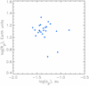 |
Fig. 7 Distribution of selected transiting KOI targets (listed in Table 1) over their radii, Rp, and orbital semimajor axes ap, according tothe NASA EA (https://exoplanetarchive.ipac.caltech.edu/). |
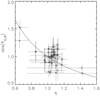 |
Fig. 8 Consistency indexes |Xs,e| and η for the transit parameter sets of selected KOI targets (listed in Table 1). Squares and crosses mark the indexes, which were found using the ingress and egress parts of the TLSs, respectively. The indexes uncertainties are shown as error bars, according the values in Table 1. To distinguish the error bars for ingress and egress symbols at the same value of η for the same object, a small artificial displacement of squares and crosses, equivalent to η ± 0.0025 is introduced. The dashed curve shows the predicted relation according to Eq. (9). |
4 Checklist
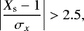
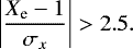
Based on the results of performed analysis, it is worth compiling a list of the most interesting targets for future studies. We use for this purpose the following criteria and select the objects with the supposed peculiar shadows:
 (14)
(14)
 (15)
(15)
 (16)
(16)
If any of the conditions in the above list of Eqs. (14)–(16) were true, the object was suspected to have an unusual shadow and was included in Table 2. Taking into account the data related problems and limitations (noted in Table 2 and discussed in Sect. 3.2), the most interesting targets in the whole considered data set are the objects orbiting around stars KIC 5794240 and KIC 11517719. Their high-quality derivatives (due to the low impact parameters β ≤ 0.144) reliably reveal the elliptical shadows, which are stretched along the X-axis, or approximately in the orbital plane.
We note that the simulation in Fig. 12a does not reproduce the elongation of the shadow of the transiting object Kepler-45b at KIC 5794240 in Fig. 10a. In fact, the effect of elongation of shadow in Fig. 10a was decreased to a certain degree by applying the correcting coefficient 1∕K = 0.79, according to Eqs. (2) and (5). This coefficient K = 0.5(|Xs| + |Xs|) was determined by the elongation effect, which appeared in the shadow in Fig. 12a, which was reconstructed from the simulated TLC. In many cases, such a correction removes the major distortions of the shadow that are caused by limb-darkening and successfully restores the circular planetary disks, as shown in Fig. 9. However, in the case of Kepler-45b at KIC 5794240, there is an additional elongation of the shadow, which cannot be corrected via the coefficient K and it appears as a novel unpredicted feature.
Since, in the case of Kepler-45b at KIC 5794240, there is a sign of inconsistency, expressed via 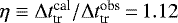 , the transit duration,
  , as well as the proportional time scale, TR, are overestimated because the applied parameter, ap, from the NASA EA, and the proportional orbital velocity, appear to be underestimated. Hence, Eq. (2) underestimates the values |Xs,e|∝ 1∕TR. In the standard model of a spherical transiting planet with a circular shadow, we can predict that this underestimation should be manifested as |Xs,e| < 1. However, we can see that |Xs| = 1.21 and |Xe | = 1.14 (in Table 1). These unpredictable excess of values |Xs, e| > 1 argues in favor of an additional lengthening of the transiter’s body, which is even higher than that shown in Fig. 10a.
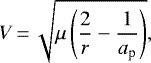
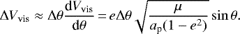
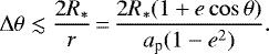
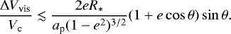
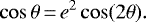
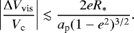
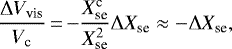
The possibility of distortion of an exoplanetary silhouette due to the orbital eccentricity, e, should be addressed additionally. Such a distortion is related to the varying visible speed, Vvis, of a planetary shadow (i.e., projected velocity) on the stellar disk. Equation (B.13) allows for an estimation of an upper limit of the effect of eccentricity in Xse. For a typical hot Jupiter value of R*∕ap ~ 0.1, Eq. (B.13) gives the maximal distortion 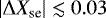 for e = 0.3 and
 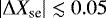 for e = 0.4. These values are below the resolution of XY -diagrams that is achieved with the silhouette reconstruction method on the basis of derivative D, as, for example, in Figs. 9–11, and 13. We note that the maximal eccentricity in our data set is
 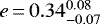 for KOI 12.01 that is orbiting KIC 5812701. Moreover, due to the strong tidal interaction with their host stars, hot Jupiters usually have even smaller eccentricities, namely, e < 0.2 (Wang et al. 2017). Therefore, the eccentricity effect is unlikely to produce detectable distortions in the XY -diagrams.
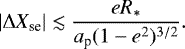
Another factor of possible distortion of planetary shadows is the tidal interaction of planet with its parent star. Using the inequality (Eq. (C.4)) from Appendix C, we can estimate the maximal aspect ratio (Xe− Xs)∕(Ymax − Ymin) of the planetary shadow. In the case of KOI 203.01 orbiting KIC 10619192, which has in our dataset the minimal value of ap = 0.026 a.u., we obtain (with the parameters from NASA EA and taking into account β = 0.105) that cos ϑ ≈ R*∕ap = 0.18. Finally, this gives us (Xe− Xs)∕(Ymax − Ymin) < 1.09 for the Love number h2 = 2.5 (in the case of a homogeneous liquid sphere) and (Xe− Xs)∕(Ymax − Ymin) < 1.06 for a more realistic h2 = 1.4 (Hellard et al. 2020) with the corresponding amax = 1.14b, cmin = 0.95b, as defined in Appendix C. The deviations <0.09 and <0.06 of the obtained aspect ratio values from unit, which corresponds to the spherical case, appear below the resolution limit > 0.1 of XY -diagrams along X-axis in Figs. 9–11, and 13. Since the tidal deformation of other (more distant from their parent stars) objects in our data set should be weaker, we draw a conclusion regarding the non-detectability of the tidal deformation signatures in XY -diagrams of planetary shadows.
 |
Fig. 9 Reconstruction of circular shadows of some exoplanets, using the real TLCs. Panel a: Kepler-1b at KIC 11446443, panel b: Kepler-12b at KIC 11804465, panel c: Kepler-17b at KIC 10619192, and panel d: Kepler-422b at KIC 9631995. The solid curves are the polynomial approximations according to Eq. (10). |
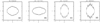 |
Fig. 10 Reconstruction of elongated shadows of some exoplanets, using the real TLCs. Panel a: Kepler-45b at KIC 5794240, panel b: Kepler-840b at KIC 11517719, panel c: Kepler-670b at KIC 11414511, and panel d: Kepler-6b at KIC 10874614. The solid curves are the polynomial approximations according to Eq. 10). |
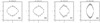 |
Fig. 11 Reconstruction of rhomboidal shadows for some exoplanets, using the real TLCs. Panel a: Kepler-8b at KIC 6922244, panel b: Kepler-448b at KIC 5812701, panel c: Kepler-5b at KIC 8 191 672, and panel d: Kepler-13b at KIC 9941662. The solid curves are the polynomial approximations according to Eq. (10). |
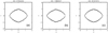 |
Fig. 12 Rhomboidal shadows reconstructed from the synthetic TLCs generated for the spherical models of some transiting objects. Panel a: Kepler-45b at KIC 5794240, panel b: KOI 883.01 at KIC 7380537, panel c: Kepler-5b at KIC 8191672, and panel d: Kepler-5b at KIC 8191672. The solid curves are the polynomial approximations according to Eq. (10). We note that the obtained shadows are elongated along X axis because the parameter K, related to limb-darkening in Eq. (5), is taken as equal to the unit. |
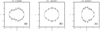 |
Fig. 13 Asymmetric (vs. X) shadows, reconstructed for some exoplanets, using the real TLCs. Panel a: Kepler-7b at KIC 5780885, panel b: Kepler-488b at KIC 10904857, panel c: Kepler-71b at KIC 9595827. The solid curves are the polynomial approximations according to Eq. (10). |
5 Conclusions
The new method of probing the transiting planet’s shape proposed in this study is applicable to the verification of an a priori expected circular form of the transiting shadows, as those shown in Fig. 9, over the wide range of the impact factor values of 0.07 ≤ β ≤ 0.82. However, a noticeable specific rhombus-like distortion of the shadow might take place in some cases (Fig. 11), which is also reproduced in the simulations as an effect of limb-darkening (Fig. 12). The high level of noise in some TLCs is the main limiting factor leading to the asymmetric (i.e., unstable) solutions for the small transiting objects.
Nevertheless, several unusual object cases were identified based on their possibly peculiar shadows. These objects are listed in Table 2. Of particular interest among them are the planets Kepler-45b and Kepler-840b, orbiting the stars KIC 5794240 and KIC 11517719, respectively. Figures 10a and b shows their elliptical shadows, which are notably elongated by ≈18% and ≈41% along the transit trajectories, in other words, approximately in the orbital planes. Formally, this geometry of shadows’ shape could be caused by exorings that are inclined to the orbital planes. Such configurations are, however, unstable and highly variable because of the Lidov-Kozai effect due to the perturbations, caused by the host star (Sucerquia et al. 2017). Our previous studies of the elongated and varying shadows of transiting hot Jupiters (Arkhypov et al. 2020) are consistent with this scenario. In particular, the TLC of transiting object at KIC 11517719 has a detectable variability of the borders, which indicates the variability of the object’s shadow (see Table 2 in Arkhypov et al. 2020). Another explanation of the elongated shadows may be that there are dynamical dusty envelopes around the planets, which are probably related to escaping planetary material interacting with the entire medium.
Less reliable cases of peculiar shadows are suspected for five objects, as shown in Table 2. Unfortunately, the noisy TLCs of four of them make a more precise analysis difficult. The remaining case of KIC 9941662 allows for an improvement, if a better measurement of the stellar radius and surface gravity would be available.
The numerical simulations (e.g., in Figs. 4–6, and 12) illustrate the high potential of the proposed approach for the diagnostics of exoplanetary environments and the possible revealing of dust envelopes and exorings, as well as for checking of the related inconsistencies of the transit parameters.
In summary, we confirm the applicability of the proposed approach and obtained results to the data provided by ongoing and future space missions with high-precision stellar photometry, such as TESS, CHEOPS, PLATO, etc. Even a non-detection of the non-circular peculiarities in planetary shadows, revealed over the course of the new transit observations, could be of interest as an empirical test of the hypothetic expectation of exorings (e.g., Heising et al. 2015; Aizawa et al. 2017; Sucerquia et al. 2020). Moreover, the already discovered circumplanetary dust phenomena (Arkhypov et al. 2019, 2020) ought to be studied using the new data and methods that are becoming available.
Acknowledgements
The authors acknowledge the projects I2939-N27 and S11606-N16 of the Austrian Science Fund (FWF) for the support.M.L.K. is grateful also to the grant No.075-15-2020-780 (GA No.13.1902.21.0039) of the Russian Ministry of Education and Science and acknowledges the project “Study of stars with exoplanets” within the grant No.075-15-2019-1875 from the government of Russian Federation.
Appendix A Modeling of a TLC
Since various shape and transparency of a transiting object are possible, a universal method of pixel-by-pixel integration (Juvan et al. 2018), suitable for any shape of transiting object, is applied to compute the corresponding TLCs. The dimming of stellar flux during transit is characterized by the part of starlight blocked by the transiting object:
 (A.1)
(A.1)
where the Cartesian coordinate system, ξ, ζ, co-centered with the stellar disk with ξ-axis along the planet orbit projection on the stellar disk is used; Is is radiation intensity at a given position (ξ, ζ) on the visible stellar disk, and I is the intensity at the same position, but disturbed by the transiter. The above mentioned integrals can be replaced by sums over Np pixels with serial number i in the identical sets:
 (A.2)
(A.2)
The stellar limb-darkening is taken into account according to the best (four coefficients) approximation by Claret & Bloemen (2011), depending on particular stellar effective temperature and gravity, adopted from the NASA Exoplanet Archive. The planetary data (radius Rp, semi-major axis ap of the orbit, impact parameter β, mid-time t0 of the first observed transit, transit period Ptr) are also taken from the NASA Exoplanet Archive.
In the applied reference system, the center exoplanetary shadow has coordinates
![\begin{equation*} \xi_{\textrm{c}}\,{=}\,a_{\textrm{p}} \sin \left [\frac{2 \pi}{P_{\textrm{tr}}} (t_{k} - t_{0})\right ],\end{equation*}](/articles/aa/full_html/2021/02/aa39050-20/aa39050-20-eq48.png) (A.3)
(A.3)
 (A.4)
(A.4)
where R* is the stellar radius from the NASA Exoplanet Archive.
In the case of the simulation presented in Fig. 5, the circumstellar matter was imitated by an opaque ring in the region 1.5 < ρ∕Rp < 2.5, inclined at ε = 6 degrees relative the direction to observer, where: ![$\rho\,{=}\,\sqrt{(\xi - \xi_{\textrm{c}})^{2} + [(\zeta - \zeta_{\textrm{c}})/\sin \varepsilon ]^{2}}$](/articles/aa/full_html/2021/02/aa39050-20/aa39050-20-eq50.png) is the planetocentric distance of the stellar disk pixel projection on the ring plane.
is the planetocentric distance of the stellar disk pixel projection on the ring plane.
The time step for the calculation of ΔF was adopted as 0.02 days. This value is about 29 times of the real time step in the used short-cadence light curves, but in the modeling this enabled saving of the computational time. During the short-cadence exposition of one minute, which is typically ~ 0.7% of the transit duration, we neglect the planetary orbital motion at the short-cadence time scale. Therefore, the obtained synthetic light curve is not smoothed, appearing as a sequence of discrete counts with the short-cadence time step. The synthetic data are treated further with the same processing pipe-line as the real light curves (for details see in Arkhypov et al. 2019). As a result the synthetic folded TLC is generated.
Appendix B Orbital eccentricity influence
A non-zero eccentricity e of planetary orbit leads to the variability of visible speed Vvis of the planetary shadow on the stellar disk (i.e., projected velocity) during the transit:
 (B.1)
(B.1)
is the instantaneous orbital speed of a planet at a given point in its trajectory, or so-called vis-viva equation (Lissauer & de Pater 2019). Here μ = GM* is the standard gravitational parameter of the orbited star with the mass M*, G is the gravitational constant, and r is the distance between the two bodies. We note that the planetary mass mp is assumed to be much less than M*. According to the equation of orbit:
 (B.3)
(B.3)
where θ is the angle between the planetary radius-vector r and the axis of periapsis. The cosine of flight path angle ϕ is
 (B.4)
(B.4)
Substituting Eqs. (B.2)–(B.4) in (B.1), we obtain:
 (B.5)
(B.5)
The variation of Vvis can be expressed using the derivative:
 (B.6)
(B.6)
Taking into account that the transit path of planet across the stellar disk is ≲ 2R*, we get:
 (B.7)
(B.7)
Substituting Eq. (B.7) in Eq. (B.6) and normalizing ΔVvis to the speed  of a circular orbital motion, we find:
 (B.8)
(B.8)
The maximal variations ΔVvis∕Vc ≡ ζ correspond to the zero derivative dζ∕dθ = 0 provided by the condition:
 (B.9)
(B.9)
In the approximation of small e, the solution of Eq. (B.9) is θ = ±π∕2. In this case Eq. (B.8) gives the upper limit:
 (B.10)
Since Xse ∝ 1∕Vvis, we can write the following proportion:
 (B.11)
where index “c‘’ corresponds to the circular planetary orbit with e = 0. After inversion and derivation, Eq. (B.11) yields
 (B.12)
where  for a spherical planet (according to normalization), Xse is supposed to be not far from unit, and ΔXse is the distortion of a-priori circular planetary shadow due to the speed variation ΔVvis. Taking into account Eq. (B.10), we can write:
 (B.13)
Since Xse corresponds to Δθ∕2 in Eq. (B.7), the factor of 2 is omitted in Eq. (B.13). As a result, Eq. (B.13) can be used as an upper limit estimation of the distortion due to the orbital eccentricity of a spherical planet.
Appendix C Tidal influence
The shadow of planetary ellipsoid, deformed by tidal force of the parent star, can be described as an ellipse. The maximal elongation of such tidally distorted planetary silhouette in XY -diagrams, as that in Fig. 9, could be noticeable in central transits of hot Jupiters. Using the equations given in Correia (2014), we can estimate the maximal aspect ratio of the planetary shadow in the case of inclination angle i = π∕2 (the angle between the line of sight and the normal to the orbital plane) as follows:
 (C.1)
(C.1)
where: ϑ = − arccos(R*∕ap) the position angle of planet on its orbit at the moment of ingress/egress, measured from the sky plane in the direction to the line of sight; A and C are the inverted squares of semi-axes of the shadow ellipse, according to Eqs. (20) and (22) in Correia (2014); a = b(1 + 3q) is a semi-axis of the planetary ellipsoid directed to the parent star; b and c = b(1 − q) are the planetary ellipsoid semi-axes directed along the orbit and perpendicular to orbital plane, respectively. The parameter q is defined as follows:
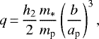 (C.2)
(C.2)
where M* and mp are the stellar and planetary masses, respectively; and h2 is the second Love number for radial displacement. A theoretical maximum of this Love number is h2 = 2.5, corresponding to the case of a homogeneous liquid sphere. The first empiric estimation of 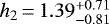 was made for the hot Jupiter WASP-121b (Hellard et al. 2020).
Altogether, Eq. (C.2) predicts that the closer to the star is the planet, the greater is difference between the semi-axes a = b(1 + 3q) and c = b(1 − q) of the planetary ellipsoid. However, there is an upper limit value for q, which corresponds to the Roche limit (Chandrasekhar 1987):
 (C.3)
(C.3)
Substituting Eq. (C.3) instead of ap in Eq. (C.2), we obtain the maximal value ![$q_{\textrm{max}}\,{=}\,h_{2}/[2 (2.46)^{3}]\approx h_{2}/30$](/articles/aa/full_html/2021/02/aa39050-20/aa39050-20-eq70.png) . The corresponding upper limits for the planetary ellipsoid semi-axes are amax = b(1 + 3qmax) = 1.25b and cmin = b(1 − qmax) = 0.92b for the maximal Love number h2 = 2.5 (Correia 2014). For such an upper-limit case, Eq. (C.1) gives the inequality:
. The corresponding upper limits for the planetary ellipsoid semi-axes are amax = b(1 + 3qmax) = 1.25b and cmin = b(1 − qmax) = 0.92b for the maximal Love number h2 = 2.5 (Correia 2014). For such an upper-limit case, Eq. (C.1) gives the inequality:
 (C.4)
(C.4)
This inequality (Eq. (C.4)) can be used for the estimation of tidal distortions of the planetary shadows.
References
- Aizawa, M., Uehara, S., Masuda, K., Kawahara, H., & Suto, Ya. 2017, AJ, 153, 193 [NASA ADS] [CrossRef] [Google Scholar]
- Aizawa, M., Masuda, K., Kawahara, H., & Suto, Y. 2018, AJ, 155, 206 [NASA ADS] [CrossRef] [Google Scholar]
- Akinsanmi, B., Santos, N. C., Faria, J. P., et al. 2020, A&A, 635, L8 [NASA ADS] [CrossRef] [EDP Sciences] [Google Scholar]
- Arkhypov, O. V., Khodachenko, M. L., & Hanslmeier, A. 2019, A&A, 631, A152 [NASA ADS] [CrossRef] [EDP Sciences] [Google Scholar]
- Arkhypov, O. V., Khodachenko, M. L., & Hanslmeier, A. 2020, A&A, 638, A143 [NASA ADS] [CrossRef] [EDP Sciences] [Google Scholar]
- Biersteker, J., & Schlichting, H. 2017, AJ, 154, 164 [NASA ADS] [CrossRef] [Google Scholar]
- Claret, A., & Bloemen, S. 2011, A&A, 529, A75 [NASA ADS] [CrossRef] [EDP Sciences] [Google Scholar]
- Chandrasekhar, S. 1987, Ellipsoidal Figures of Equilibrium (New York: Dover) [Google Scholar]
- Correia, A. C. M. 2014, A&A, 570, L5 [NASA ADS] [CrossRef] [EDP Sciences] [Google Scholar]
- Esteves, L. J., De Mooij, E. J. W., & Jayawardhana, R. 2013, ApJ, 772, 51 [NASA ADS] [CrossRef] [Google Scholar]
- Heising, M. Z., Marcy, G. W., & Schlichting, H. E. 2015, ApJ, 814, 81 [NASA ADS] [CrossRef] [Google Scholar]
- Hellard, H., Csizmadia, S., Padovan, S., Sohl, F., & Rauer, H. 2020, ApJ, 889, 66 [NASA ADS] [CrossRef] [Google Scholar]
- Huber, D., Silva Aguirre, V., Matthews, et al. 2014, ApJS, 211, 2 [NASA ADS] [CrossRef] [Google Scholar]
- Jackson, B., Adams, E., Sandidge, W., Kreyche, S., & Briggs, J. 2019, AJ, 157, 239 [CrossRef] [Google Scholar]
- Juvan, I. G., Lendl, M., Cubillos, P. E., et al. 2018, A&A, 610, A15 [NASA ADS] [CrossRef] [EDP Sciences] [Google Scholar]
- Kenworthy, M. A., & Mamajek, E. E. 2015, ApJ, 800, 126 [NASA ADS] [CrossRef] [Google Scholar]
- Kepler Mission Team. 2009, VizieR On-line Data Catalog: V/133 [Google Scholar]
- Li, J., Tenenbaum, P., Twicken, J. D., et al. 2019, PASP, 131, 024506 [NASA ADS] [CrossRef] [Google Scholar]
- Lissauer, J. J., & de Pater, I. 2019, Fundamental Planetary Sciences (New York: Cambridge University Press) [Google Scholar]
- Mathur, S., Huber, D., Batalha, N. M., et al. 2017, ApJS, 229, 30 [NASA ADS] [CrossRef] [Google Scholar]
- Pass, E. K., Cowan, N. B., Cubillos, P. E., & Sklar, J. G. 2019, MNRAS, 489, 941 [CrossRef] [Google Scholar]
- Sliski, D., & Kipping, D. M. 2014, ApJ, 788, 148 [NASA ADS] [CrossRef] [Google Scholar]
- Sandford, E., & Kipping, D. 2019, AJ, 157, 42 [NASA ADS] [CrossRef] [Google Scholar]
- Sucerquia, M., Alvarado-Montes, J. A., Ramírez, V., & Zuluaga, J. I. 2017, MNRAS, 472, L120 [NASA ADS] [CrossRef] [Google Scholar]
- Sucerquia, M., Alvarado-Montes, J. A., Zuluaga, J. I., Montesinos, M., & Bayo, A. 2020, MNRAS, 496, 85 [Google Scholar]
- Wang, Y., Zhou, J.-l., Hui-gen, L., & Meng, Z. 2017, ApJ, 848, 20 [NASA ADS] [CrossRef] [Google Scholar]
- Zuluaga, J. I., Kipping, D. M., Sucerquia, M., & Alvarado, J. A. 2015, ApJ, 803, L14 [NASA ADS] [CrossRef] [Google Scholar]
All Tables
All Figures
|
Fig. 1 Example of TLC proximity for different transit geometries. Panel a: model of a spherical object with β = 0.796 and ap = 0.032 au; panel b: model of an elongated disk-type shape of the transiting shadow (a thin disk with an increased radius of 2.59 times of that in the case of mode (a) and tilt of 6.38 deg.), keeping the same depth of TLC minimum, with β = 0.054 and ap = 0.053 au; panelc: combination of synthetic TLCs calculated for the models (a) (dashed line) and (b) (solid line). The orbital period and stellar parameters are the same in both models. Here, ΔF is the decrease of the radiation flux caused by the transiting object. The abscissa parameter Δt is the time relative to the predicted transit mid-time. |
| In the text | |
|
Fig. 2 Example of a KOI 1.01. Panel a: folded TLC; panel b: derivatives of the TLC’s ingress (squares) and egress (crosses) parts. The analyzed part of the derivative is marked in red. |
| In the text | |
|
Fig. 3 Moving, co-centered with planet, orthogonal coordinate system (X, Y), used for the calculation of D. The planetary disc (blue circle), with the center of coordinate “C”, obscures the stellar disk (yellow segment), moving across it with the projected velocity V (red vector). The X-axis is pointed to the center of stellar disc, for the egress (right panel), and opposite, for the ingress (left panel) phases, respectively. |
| In the text | |
|
Fig. 4 Trial reconstruction of transiter’s silhouette (bottom panel) of Kepler-1b at KIC 11446443, using the synthetic TLC simulated for a spherical transiter with the radius and transit geometry of the planet taken from NASA EA. Vertical bars in the restored silhouette depict its uncertainty (± standard error). The simulated transit geometry, used for the calculation of K-factor in Eq. (5), is illustrated in upper panel. The horizontal solid line shows the trajectory of transiter across the stellar disk. |
| In the text | |
|
Fig. 5 Model of transiting object with a ring (upper panel), built on the basis of the real object KIC11446443, to simulate TLC of a ringed planet. The total area of obscuration is the same as in Fig. 4. The reconstructed silhouette (bottom panel), obtained from the synthetic TLC reveals the presence of the distorting structure. |
| In the text | |
|
Fig. 6 Transiter model with a halo (upper panel), built on the basis of real object KIC11446443. The total area of obscuration is the same as in Fig. 4. The reconstructed silhouette (bottom panel), obtained from the synthetic TLC reveals the distortion of the circular shape of planetary shadow. |
| In the text | |
|
Fig. 7 Distribution of selected transiting KOI targets (listed in Table 1) over their radii, Rp, and orbital semimajor axes ap, according tothe NASA EA (https://exoplanetarchive.ipac.caltech.edu/). |
| In the text | |
|
Fig. 8 Consistency indexes |Xs,e| and η for the transit parameter sets of selected KOI targets (listed in Table 1). Squares and crosses mark the indexes, which were found using the ingress and egress parts of the TLSs, respectively. The indexes uncertainties are shown as error bars, according the values in Table 1. To distinguish the error bars for ingress and egress symbols at the same value of η for the same object, a small artificial displacement of squares and crosses, equivalent to η ± 0.0025 is introduced. The dashed curve shows the predicted relation according to Eq. (9). |
| In the text | |
|
Fig. 9 Reconstruction of circular shadows of some exoplanets, using the real TLCs. Panel a: Kepler-1b at KIC 11446443, panel b: Kepler-12b at KIC 11804465, panel c: Kepler-17b at KIC 10619192, and panel d: Kepler-422b at KIC 9631995. The solid curves are the polynomial approximations according to Eq. (10). |
| In the text | |
|
Fig. 10 Reconstruction of elongated shadows of some exoplanets, using the real TLCs. Panel a: Kepler-45b at KIC 5794240, panel b: Kepler-840b at KIC 11517719, panel c: Kepler-670b at KIC 11414511, and panel d: Kepler-6b at KIC 10874614. The solid curves are the polynomial approximations according to Eq. 10). |
| In the text | |
|
Fig. 11 Reconstruction of rhomboidal shadows for some exoplanets, using the real TLCs. Panel a: Kepler-8b at KIC 6922244, panel b: Kepler-448b at KIC 5812701, panel c: Kepler-5b at KIC 8 191 672, and panel d: Kepler-13b at KIC 9941662. The solid curves are the polynomial approximations according to Eq. (10). |
| In the text | |
|
Fig. 12 Rhomboidal shadows reconstructed from the synthetic TLCs generated for the spherical models of some transiting objects. Panel a: Kepler-45b at KIC 5794240, panel b: KOI 883.01 at KIC 7380537, panel c: Kepler-5b at KIC 8191672, and panel d: Kepler-5b at KIC 8191672. The solid curves are the polynomial approximations according to Eq. (10). We note that the obtained shadows are elongated along X axis because the parameter K, related to limb-darkening in Eq. (5), is taken as equal to the unit. |
| In the text | |
|
Fig. 13 Asymmetric (vs. X) shadows, reconstructed for some exoplanets, using the real TLCs. Panel a: Kepler-7b at KIC 5780885, panel b: Kepler-488b at KIC 10904857, panel c: Kepler-71b at KIC 9595827. The solid curves are the polynomial approximations according to Eq. (10). |
| In the text | |
Current usage metrics show cumulative count of Article Views (full-text article views including HTML views, PDF and ePub downloads, according to the available data) and Abstracts Views on Vision4Press platform.
Data correspond to usage on the plateform after 2015. The current usage metrics is available 48-96 hours after online publication and is updated daily on week days.
Initial download of the metrics may take a while.