| Issue |
A&A
Volume 645, January 2021
|
|
|---|---|---|
| Article Number | A136 | |
| Number of page(s) | 10 | |
| Section | Atomic, molecular, and nuclear data | |
| DOI | https://doi.org/10.1051/0004-6361/202039685 | |
| Published online | 28 January 2021 | |
Spectral properties and polarizabilities for fluorine-like ions with Z = 20–30★
School of Physics and Information Technology, Shaanxi Normal University, Xi’an 710119, PR China
e-mail: This email address is being protected from spambots. You need JavaScript enabled to view it.
Received:
15
October
2020
Accepted:
16
November
2020
Abstract
Aims. The primary motivation of this paper is to provide accurate atomic properties of F-like ions with Z = 20−30, including energy levels, line strengths, static dipole polarizabilities, and lifetimes. In addition, a detailed analysis is also carried out to explore the convergence and uncertainties of our results.
Methods. Large-scale B-spline relativistic configuration interaction calculations are carried out to generate the atomic properties of F-like ions. The radial parts of one-electron Dirac orbitals are obtained from the relativistic self-consistent field procedure in which the Breit Interaction and QED corrections (vacuum polarization and self-energy terms) are also included. A numerical method, called Emu CI, is adopted to decrease the size of CI matrix significantly without loss of much accuracy.
Results. Energy levels and line strengths for electric-dipole (E1), electric-quadrupole (E2), and magnetic-dipole (M1) transitions are provided for the 250 lowest levels of each system, showing a good agreement with available theoretical and experimental information. The static dipole polarizabilities and lifetimes for the ten lowest states are also reported. A statement for the convergence and uncertainties of our results is presented.
Key words: atomic data / atomic processes / relativistic processes / methods: numerical
Full Tables 1 and A.1, and the transition line strengths of all the ions are only available in electronic format at the CDS via anonymous ftp to cdsarc.u-strasbg.fr (130.79.128.5) or via http://cdsarc.u-strasbg.fr/viz-bin/cat/J/A+A/645/A136
© ESO 2021
1 Introduction
Highly charged ions (HCIs) have been of long-standing interest; not only do they provide many opportunities to study basic atomic physics, but they also have important applications in high-temperature plasma and astrophysics. Optical transitions of many HCIs are sensitive to the fine-structure constant variation (Berengut et al. 2010, 2012, 2011; Dzuba et al. 2015; Safronova et al. 2014a) and interactions with dark matter (Van Tilburg et al. 2015; Stadnik & Flambaum 2014), and they can also be used to build high-accuracy atomic clocks (Safronova et al. 2014a,b; Derevianko et al. 2012; Dzuba et al. 2013). In plasma diagnostics, combined with the corresponding data sets of various collision strengths, spectral lines of HCIs can provide some important properties, such as ionization state, elemental abundances, electron temperature, and density (Warren et al. 1997; Clementson & Beiersdorfer 2013; Zanna 2006). As an important part of HCIs, the spectra of medium-Z F-like ions, especially the iron period elements, can often be observed in both astrophysical (Curdt et al. 2004; Landi & Phillips 2005; Shestov et al. 2013) and laboratory plasmas (Safronova et al. 2012; Gu et al. 2007a,b; Ouart et al. 2011). For example, the magnetic-dipole transitions 2s22p5 2P3∕2 − 2s22p5 2P1∕2 for F-like Fe and Ni ions are often measured and studied in tokamaks to help determine ion temperatures (Hinnov & Suckewer 1980), the spectral lines of Fe XVIII in far-ultraviolet spectroscopy have been detected in the binary system Capella (Young et al. 2001), and the extreme ultraviolet (EUV) spectral lines of various F-like ions have been observed in the corona and outer atmosphere of the Sun (Doschek & Feldman 2010). A comprehensive and accurate determination of the atomic data of medium-Z F-like ions is thus of special significance in the astrophysical line interpretation and plasma modeling.
To match this interest for the atomic properties of F-like ions, there were a number of measurements reported in past decades. Reader (1982) and Reader et al. (1986) used laser irradiated solid targets to measure the transition energies of ions from Sr29+ to Sn41+. Träbert et al. (1999a,b) measured the forbidden transition rates in F-like titanium and scandium in heavy-ion storage rings. More recently, F-like tungsten was measured by Podpaly et al. (2009) using the high-resolution flat-crystal spectrometer on the SuperEBIT electron beam ion trap. A wealth of theoretical studies were reported in the new century due to the great advance in computing power. Jonauskas et al. (2004) calculated the excitation energies of the 379 lowest bound levels and multipole transition probabilities for Fe XVIII using the multi-configuration Dirac-Fock (MCDF) method. The same method was utilized by Jönsson et al. (2013) to produce transition energies and transition rates of the 2s22p5 configuration for F-like ions from Si VI to W LXVI. Gu (2005) calculated the energies of 1s22lp states for Z ≤ 60 with a combined configuration interaction and many-body perturbation theory approach. Nahar (2006) reported the allowed and forbidden transitions in Fe XVIII using the relativistic Breit-Pauli R-matrix method. Most of these calculations focused on a single ion, mostly Fe XVIII, or on some low-lying states of different ions. It is clear that a complete data set for different F-like ions including the high-lying states of n = 3, 4 configurations is important on account of their wide applications. Froese Fischer & Tachiev (2004) performed acomprehensive study for the energy levels and transition characteristics for F-like ions with Z = 9−22, in which a multi-configuration Hartree-Fock (MCHF) code is adopted, and the relativistic effects are also taken into account through a Breit-Pauli Hamiltonian. Their predicted energy levels probably exhibit the best agreement to date with the observed data; however, their research is limited to the 60 lowest levels of the 2s2 2p5, 2s2 2p6, and 2s2 2p43l configurations. More recently, the 200 lowest energy levels and transition properties for F-like ions with Z = 24−30 and Z = 31−35 have been reported by Si et al. (2016) and Li et al. (2019), respectively, using MCDHF and second-order MBPT methods. Aggarwal (2019) also performed a comprehensive study of the F-like ions with Z = 12−23 using the flexible atomic code (FAC) and the general purpose relativistic atomic structure package (GRASP) code. These data sets are of comparable high accuracy; however, the agreements with other theoretical calculations and the observed data are still not satisfactory for some important levels. More accurate and complete energy levels and transition characteristics of F-like ions are expected. On the other hand, the observed data show larger uncertainties, while the uncertainties are not stated in most of the theoretical studies. Considering that various approximations, such as the frozen-core approximation and the treatment for the quantum electrodynamics (QED) effect, are essential in the calculation due to the limitation of computing resources, an analysis of the uncertainties induced by different approximations, as well as a discussion for the convergence of calculations, is also of great importance.
The primary motivation of the present work is to provide a consistent and accurate data set of energy levels and transition characteristics for F-like ions with Z = 20−30 via large-scale B-spline relativistic configuration interaction calculations. A numerical method, called Emu CI, for decreasing the size of the CI matrix is adopted to effectively minimize the computational resources without undermining much accuracy. Energy levels for the 250 lowest levels, as well as multipole transition line strengths (electric dipole, quadrupole, and magnetic dipole), static electric dipole polarizabilities, and lifetimes for the ten lowest levels of each ion are reported. Meanwhile, a detailed analysis is also carried out to explore the convergence and uncertainties of our results. The package we used is the Ambit code by Kahl & Berengut (2019).
2 Theory and calculation
2.1 Particle-hole CI
The no-pair Dirac-Coulomb Hamiltonian is taken as our Hamiltonian (Sucher 1980),
![Mathematical equation: \begin{equation*} H\,{=}\,\sum_{i\,{=}\,1}^{N}\left [c \boldsymbol{ \alpha \cdot \mathit{p} }+(\beta -1)c^2 - V{_{i}^{N}} \right]+\sum_{i< j}^{N}\frac{e_{i}e_{j}}{r_{ij}}, \end{equation*}](/articles/aa/full_html/2021/01/aa39685-20/aa39685-20-eq1.png) (1)
(1)
where c is the speed of light, α and β are Dirac matrices, and p is the momentum operator. The potential  is the electron–nucleus Coulomb interaction, where a point-charge model for the nuclear charge distribution is adopted, and the uncertainty introduced is discussed in a later section. The atomic state wave functions are given by linear expansions of configuration state wave functions (CSF),
 (2)
(2)
In this expression P is the parity, J and M are the angular momentum quantum numbers, and γ denotes other appropriate labels of the CSF. The CSFs are built from antisymmetrized and coupled products of one-electron Dirac orbitals. The radial parts of the one-electron Dirac orbitals are obtained from the relativistic self-consistent field (RSCF) procedure and constructed as a linear combination of 50 B-spline basis functions of order k = 7. The Breit interaction (Johnson 2007),
![Mathematical equation: \begin{equation*} H_{Breit} \,{=}\, -\sum_{i<j}^{N} \frac{1}{2r_{ij}} \left [\alpha_{i} \cdot \alpha_{j} +\frac{\left (\alpha_{i} \cdot r_{ij} \right) \left (\alpha_{j} \cdot r_{ij} \right)}{r_{ij}^{2}} \right], \end{equation*}](/articles/aa/full_html/2021/01/aa39685-20/aa39685-20-eq4.png) (3)
(3)
and QED corrections (vacuum polarization and self-energy terms) are also included in the RSCF calculation. Eigenvalues and mixing coefficients are obtained by diagonalizing the Hamiltonian matrix. Due to the limitation of computing resources, only the configurations generated by exciting electrons from the occupied orbitals in some reference configurations to unoccupied orbitals are included in the CI expansion.
In the present work, 1s22s22p5 configuration is chosen in the relativistic self-consistent field (RSCF) calculation to generate one-electron Dirac orbitals. The 1s shell is set as a frozen core from which no electron or hole is excited. The 2p−1, 2s−1, 2p−2 3s1, 2p−2 3p1, 2s−2 3s1, 2s−2 3p1, 2s−1 2p−13s1, and 2s−1 2p−13p1 configurations are set as reference configurations. Here the complete shell is not indicated, and the subscript − n denotes n holes in the corresponding shell. For example, 2p−1 is the same as 1s22s22p5 configuration. In our calculations, the configurations like 1s22s22p5 are treated as one hole with positive charge in closed 2p shell. The uncertainties resulting from the fix of two 1s electrons are discussed later in this work. In the construction of CI matrix, single and double valence electronic excitation from 3s and 3p shells, and single and double core-hole excitation from 2s and 2p shells in thereference configurations are allowed to generate CSF sequences. The 35 lowest states of J = 0.5, 1.5, 2.5, 3.5, 4.5 in both even and odd parities are calculated, and the largest matrix is built for J = 5∕2, which has 134 036 CSFs.
2.2 Emu CI
The size of the Hamiltonian matrix expands rapidly with the increasing number of electrons included in the CI calculation, resulting in a large occupation of computational resources. However, in the common case for the energy levels that are indeed needed, their CI expansions are always dominated by the CSFs with close energies. Higher-energy CSFs contribute less strongly, and the interactions between these CSFs are reasonably negligible. Thus, we can set the matrix elements of this part to zero without serious loss of accuracy and save a great deal of computational resources (Geddes et al. 2018).
As shown in Fig. 1, assuming there are N CSFs to be included in the CI calculation, there are M important CSFs that should be included and N − M CSFs whose contributions are expected to be negligible. Then the interaction matrix elements among these N − M configurations are set to zero, and only the matrix elements involving the M important CSFs need to be calculated. The sides consisting of N CSFs and M CSFs are termed “large side” and “small side” of the matrix, respectively, and this treatment for the CI matrix is termed Emu CI. In our calculations, the small side CSFs are built using similar settings of the large side, but only one single core-hole excitation is allowed. For example, the 2p−33p2 configuration generated by single core-hole excitation from reference configuration 2p−2 3p1 was included in the large side and the small side, but the double core-hole excitation configuration 2p−4 3p3 was only included in the large side. Using this technique, the final matrix of J = 5∕2 has 134 036 CSFs in the large side and 14 061 CSFs in the small side. A discussion of the error introduced is presented in the following section.
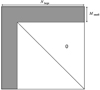 |
Fig. 1 Schematic of the Emu CI approximation. The white part represents the terms neglected in this method. Effective CI matrix elements are shaded in gray. |
2.3 Transition parameters
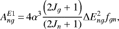
The multipole transition parameters can be expressed in terms of reduced transition matrix elements. Using the atomic units, the transition rates Agn, oscillator strengths fgn, and line strengths Sgn for electric dipole transitions from state n to state g can be calculated as
 (4)
(4)
 (5)
(5)
 (6)
(6)
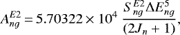
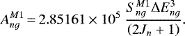
where ΔEng = En − Eg, α is the fine structure constant, and  are the spherical tensor of rank 1. For higher-order multipole transition, Sgn can be obtained by replacing the transition operator by either the magnetic dipole moment operator or the electric quadrupole moment operator, and transition probabilities can be calculated as (Safronova et al. 2001)
 (7)
(7)
 (8)
(8)
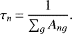
Here the transition probabilities A are given in units of s−1. Then the lifetime of a level can be computed as
 (9)
(9)
In the present work, the line strengths of all electric-dipole (E1), electric-quadrupole (E2), and magnetic-dipole (M2) transitions involving the ten lowest levels for each system are reported, and the transition rates, oscillator strengths, and lifetimes can easily be generated from the data provided in our work.
2.4 Static electric polarizabilities
Electric polarizability for a relevant quantum state of an atom or ion plays a central role in describing the interactions with an external electric field; for example, the external force and energy shift of the ions in an optical trap are mainly dependent on its polarizability coupling with the oscillating electric field. Therefore, an accurate determination of polarizabilities for the low-lying states of atoms and ions has wide applications in different areas, such as the design of high-accuracy optical clocks (Safronova et al. 2014a). Furthermore, the polarizability is also directly related to the relativistic corrections to the bound states and fine-structure intervals of Rydberg states (Bhatia & Drachman 1999, 1997), and the optical properties of inert gases including the refractive index and the Verdet constant, which measures the rotation of the plane of polarization in the Faraday effect (Bhatia & Drachman 1998).
The static electric dipole polarizabilities for a state with non-zero angular momentum J is defined as
 (10)
(10)
The quantity α0,d is called the scalar dipole polarizability, while α2,d is the tensordipole polarizability. The tensor part of the polarizability indicates its dependence on the polarization of the electric field with respect to the quantization axis of the atom or ion. The polarizabilities can be calculated using the sum-over-states approach:
 (11)
(11)
![Mathematical equation: \begin{equation*} \begin{split} \alpha _{2,d}\,{=}\,&4\left(\frac{ 5J_{g}\left(2J_{g}-1 \right) }{ 6\left(J_{g}+1 \right) \left(2J_{g}+1 \right) \left(2J_{g}+3 \right) }\right)^{\frac{1}{2}}\\[4pt] &\sum_{n} \left(-1 \right)^{J_{g}+J_{n}} \left\lbrace \begin{array}{ccc} J_{g} & 1 & J_{n} \\ 1 & J_{g} & 2 \end{array} \right\rbrace \frac{ \left | \left \langle \psi _{g} \left \| rC^{1}\left (\widehat{r} \right) \right \|\psi _{n} \right \rangle \right |^{2}}{ \Delta E_{ng} }. \end{split} \end{equation*}](/articles/aa/full_html/2021/01/aa39685-20/aa39685-20-eq14.png) (12)
(12)
In our calculations, the dipole polarizabilities of the 10 lowest levels for each system are calculated by summing over all allowed transitions in the 250 lowest levels. Furthermore, the total polarizability can be separated into the core polarizability αcore and the valence part, while our summing can only include the contribution of valence part. The 1s2core polarizabilities from Johnson et al. (1983) were added to the present scalar dipole polarizabilities, whereas the magnitudes of αcore for these ions are all approximately at a level of 10−5 au.
3 Analysis for convergence and uncertainty
The reliability and accuracy level of our calculations are directly related to the size of the basis set and configurations included in the CI calculations, and to the various approximations adopted, such as the Emu CI, the model for nuclear charge distribution, and the frozen core shell chosen. To verify the convergence of our calculations and explore the uncertainties introduced by different approximations, a number of calculations were performed and compared with each other. Some of them, such as setting the 1s2 core electrons active, are very time consuming and are only performed for Fe XVIII as a showcase.
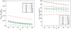 |
Fig. 2 Convergence of the 12 lowest excited states when the CI basis set is increased from 7spdfg to 8spdfg. |
3.1 Sizes of the B-spline basis and CI matrix
The convergence rate of CI calculations is expected to be achieved by a series of tests with different sizes of CI space and basis set; however, due to the practical limitation of computation resources, and because our settings are large enough compared with existing theoretical calculations, a simplified convergence test is performed in our calculations. The maximum principal quantum number n of full CI calculations is expanded from 7 to 8 and the comparisons are made for all the systems. The 12 lowest excited states are compared in Fig. 2, while a detailed comparison for the 250 lowest energy levels of Fe XVIII are displayed in Table 1. We find that the magnitude of differences for a specific state resulting from a larger CI space did not change much for different ions. The increase in CI space has a negligible effect on the first excited state for all systems with a change of no more than 1 cm −1. For the second excited state the differences are about 160 cm−1, and for other excited states the differences are mostly in the range 200−400 cm −1. The relativedifferences for a specific state decrease as the nuclear charge increases since the transition energies become larger owing to the more compact wave functions. In the case of Z = 20, most energy levels decrease by approximately 0.1o and the second excited state has changed by 0.2o, while they are only 0.03 and 0.12o when Z = 30. A convergence test for the number and order of the B-spline basis was also performed and the situation is similar. The number and order of the B-spline were expanded from 50 and 7 to 90 and 8, respectively, leading to an impact of about 2 cm −1 for the first excited state, 40 cm−1 for the second excited state, and 130 cm−1 for the other states. Finally, we give that the present calculations for the energy levels of all systems are converged within 5, 250, and 600 cm−1 for the first, second, and other excited states, respectively.
3.2 Emu CI
The uncertainties introduced by the Emu CI method, in which the interactions between configurations generated by double core-hole excitation from 2s and 2p shells are set to zero, are also investigated by a series of test calculations. In Fig. 3 Emu CI energies are compared to the full CI results for the 12 lowest excited states, and a complete data set of both Emu CI and full CI energy levels for Fe XVIII are listed in Table 1. Once again, the magnitudes of differences for a specific state are of similar sizes for different ions and the relative difference decreases as the nuclear charge increases. For the first and second excited states, the changes are less than 1 cm −1 for all the ions. The differences are larger for higher excited sates, but never exceed 130 cm−1. The changes for most of the highly excited states, such as the states belong to the 2p−2 3d1 and 2p−2 4s1 configurations, are always less than 50 cm−1. On the other hand, using the same settings of CI space, the time used by the Emu CI calculations is only one-third of the full CI calculations. These tests confirm that neglecting some specific matrix elements can significantly decreases the time and memory resources needed without having a significant impact on the accuracy compared to a standard CI calculation.
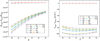 |
Fig. 3 Comparison of the present Emu CI and full CI excitation energies for the 12 lowest excited states. |
3.3 Nuclear model
In the present calculations a point-charge model for the nuclear charge distribution is adopted in the description of nuclear potential. A test using the Fermi charge distribution was also performed to explore the uncertainties introduced, but its effect was found to be minor. The resulting change in the first excited energy level is less than 0.2 cm −1, and can be ignored. The largest change occurs in the second excited state, which is about 40 cm−1. For other energy levels the changes never exceed 10 cm−1. Accordingly, the uncertainties introduced from different models for nuclear charge distribution is omitted for the first excited states, 40 cm −1 for the second excited states, and 10 cm−1 for the other states.
3.4 Frozen core approximation
In order to explore the influence of setting the 1s2 core shell frozen, we did a test in which two 1s electrons are also allowed to be excited. This makes the size of CI matrix three times as large as before, and brings in a huge consumption of computing and time resources. Due to the practical limitation, only the states of J = 0.5 for Fe XVIII were calculated. We assume that it has a similar impact on other ions. The energy of the first, second, fifth, and seventh excited states obtained in this manner are 102 596, 1 075 352, 6 300 933 and 6 342 833 cm −1, respectively. Compared with the results of our full CI calculations, setting the 1s2shell open resulted in a change of about 100 cm−1 for the first, 1000 cm−1 for the second, and 3000 cm−1 for the higher excited states, and makes differences with NIST values from 73, 11 595, 12 539, and 3067 cm −1 reduced to 17, 10 650, 9267, and 233 cm−1, respectively. This suggest that it has an important contribution to the improvement of the accuracy level of our calculations. For other systems we assume that the present CI calculations have similar uncertainties.
In summary, a series of test calculations was performed to explore the convergence of our settings and uncertainties introduced by various approximations. We conclude, for the energy levels in our calculations, that setting the maximum principal quantum number n = 7 and angular quantum number l = 4 for the CI space and using 50 B-spline bases of order 7 are converged within 5, 250, and 600 cm −1 for the first, second, and other excited states, respectively. The largest source of uncertainty in our calculation is setting the 1s2core shell frozen, leading to a uncertainty of about 100 cm−1 for the first, 1000 cm−1 for the second, and 3000 cm−1 for higher excited states. The technique of Emu CI and the point-charge nuclear model are two other important sources of uncertainties: 1 cm −1 for the first, 45 cm−1 for the second, and 140 cm−1 for the other excited states. Finally, we give that the total uncertainties of our energy levels are less than 110, 1300, and 3800 cm −1 for the first, second, and other excited states, respectively, for all the ions we calculated. The corresponding relative uncertainties decrease against the increasing of nuclear charge Z; for example, they are respectively about 0.3, 0.2, and 1.2% for Ca XII; 0.1, 0.1, and 0.5% for Fe XVIII; and 0.05, 0.1, and 0.3% for Zn XXII. In addition, the accuracy level of wavelengths and line strengths relies on the calculation of energy levels. The total uncertainty of our wavelengths and line strengths are stated as 2% for the transitions in which the first or second excited state is involved, and 3% for all other transitions. The static dipole polarizabilities and lifetimes of the ten lowest levels determined by our line strengths are also reported. The uncertainties of our predicted dipole polarizabilities are also given as 3%. Although only E1, E2, and M1 transitions are included in our calculations, the omitted transitions contribute less to the lifetimes of the nine lowest excited states that we report in the present work; therefore, the uncertainty of our listed lifetimes are given as 5%.
Energy levels (in cm−1) relative to the ground state for the 250 lowest levels of Fe XVIII.
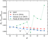 |
Fig. 4 Difference in percentage of energy levels from the present Emu CI calculations for the first excited state 2s2 2p52P1∕2 compared to those from NIST (Kramida et al. 2019) and other calculations (Si et al. 2016; Jönsson et al. 2013; Nandy & Sahoo 2014). |
4 Results and discussion
4.1 Energy levels
We performed large-scale B-spline CI calculations and reported the 250 lowest energy levels relative to the ground state of F-like ions with Z = 20−30. In Figs. 4 and 5 a comparison of our results with the NIST compiled data (Kramida et al. 2019) and other calculations (Jönsson et al. 2013; Si et al. 2016; Nandy & Sahoo 2014) are presented for the first two excited sates (2s2 2p52P1∕2 and 2s 2p62S1∕2). The most important feature is that the differences between present energies and other data sets vary smoothly along the Z sequence. One exception is the calculation from Nandy & Sahoo (2014) for the 2s2 2p5 2 P1∕2 state, which exhibits a significantly irregular behavior. Meanwhile, the non-smooth behavior of the NIST compiled data for the 2s2 2p5 2 P1∕2 state of Z = 23 and 25 suggests that the NIST data for the first excited state of V XIV and Mn XVII are possibly uncertain. Figure 6 shows the relative differences between our Emu CI results and NIST energy levels. The energies of most of the states agree within 0.15% for all ions, while the smooth variety of the differences along the Z sequences provides further support for the validity of our calculations. The second excited state 2s 2p6 2S1∕2, with a hole in 2s shell and a fulfilled 2p shell, is an outlier showing a large difference of 1.8% for Z = 20 and decreasing to 0.8% for Z = 30. Such a large difference is possibly due to the one-electron Dirac orbitals generated by the RSCF procedure based on 1s22s22p5 configuration in our calculations, which are improper for the description of the 2s 2p6 2S1∕2 state.
Due to its significance in astronomy, Fe XVIII has been very carefully studied; a detailed comparison for the 250 lowest energy levels of Fe XVIII is shown in Table 1, which is available in its entirety at the CDS. The present Emu CI and full CI energies are presented in comparison with the recent calculations by Jonauskas et al. (2004), Nahar (2006), and Si et al. (2016), and the NIST compilation (Kramida et al. 2019). The information from the CHIANTI database (Del Zanna et al. 2015) obtained by Zanna et al. through the review and assessment of line identifications from laboratory and astrophysical observations are also listed for comparison. The present excitation energies agree well with the data collected from NIST and CHIANTI databases with a difference of less than 4000 cm−1 for most of the states, which is consistent with our previous statement for the uncertainty of our calculations. The stated uncertainties of the NIST values are approximately 40 cm −1 for the first excited state and 3000 cm−1 for other states, thus most of the present Emu CI energy levels lie close to the error bar of the measurements. This level of agreement is much betterthan the calculations by Jonauskas et al. (2004) and Nahar (2006) and similar with the MCDHF calculations (Si et al. 2016). If we look into the energy levels where the present results differ from the NIST data by more than 4000 cm −1, they are separated into two different classes. The energy levels 6, 18, 113, and 179 belong to the configurations 2p−2nl1, and all the theoretical data of these levels differ from the observed data by more than 0.1%, while the present results agree with the MCDHF calculations (Si et al. 2016) within 0.03% (2300 cm −1). For the levels 3, 195, 224, and some levels between 59 and 100, these states are generated by exciting one or two 2s core electrons from the 2s22p5 ground configuration, and the present results show a difference of more than 10 000 cm−1, which is lesssatisfactory. It seems that the performance of our calculations is not good for the core excitation configurations. This is an issue we need to resolve in the future; however, one noticeable feature is that for most of these levels existing theoretical calculations are significantly different from each other. Furthermore, the NIST values and the data from CHIANTI (Del Zanna et al. 2015) also exhibit large discrepancies for many of these levels, and the present results always show a better agreement with the data from CHIANTI (Del Zanna et al. 2015). For example, NIST suggest that the energy of level 6 is 6 310 200 cm−1, but from CHIANTI it is 6 301 200 cm−1 (Del Zanna et al. 2015), and our result is 6 297 661 cm−1. A similar situation can also be found in levels 18, 69, 70, 80, and 90. Setting the 1s2core electrons active in our calculations would increase the level of accuracy significantly; however, the computation resource needed is tremendous and is beyond our limit. This will be done for some highly needed levels in the future. Generally, the existing theoretical and experimental data show reasonable agreement, but obvious discrepancies are also exhibited for some specific states, especially for some core electron excited states. More precise measurements and theoretical studies are needed as benchmarks in future line identifications.
Some energy levels of F-like ions with Z = 20−30 are listed in Table A.1 along with NIST compiled data, while a complete data set for the 250 lowest energy levels of the ions are provided at the CDS. In Table A.1 the differences with the NIST data are approximately 2500 cm−1 for most of the levels. One noticeable feature is the level identification for the fifth and seventh levels with the configuration of 2s2 2p43s. They are identified in the NIST data sets for Z = 22−25 as 4 P3∕2 for the fifth level and 2 P3∕2 for the seventh level; for Z = 26−30 they are 2 P3∕2 for the fifth level and 4 P3∕2 for the seventh level. That is a switch of identifications for both levels appearing between Z = 25 and 26; however, the suggestions from our analysis and the MCDHF calculations (Si et al. 2016) are different. The MCDHF calculations state that the terms are 2 P3∕2 for the fifth level and 4 P3∕2 for the seventh level, respectively, when Z = 24−30. Our identifications are the same as the MCDHF calculations for Z = 24−30, while for Z = 20−23 our results are the same as the NIST data sets and the FAC calculation from Aggarwal (2019). In our calculations for the fifth level, the ratio of contribution from 2P3∕2 term against that of 4 P3∕2 term increases as Z increases, and the contributions from the two terms are almost evenly matched when Z = 23 and 24. The situation for the seventh level is similar, but the ratio decreases. Therefore, the switch of identifications for the fifth and seventh levels occurs between Z = 23 and 24 in our calculations, possibly also in the MCDHF calculations (Si et al. 2016).
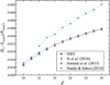 |
Fig. 5 Difference in percentage of energy levels from the present Emu CI calculations for the second excited state 2s 2p6 2 S1∕2 compared to those from NIST (Kramida et al. 2019) and other calculations (Si et al. 2016; Jönsson et al. 2013; Nandy & Sahoo 2014). |
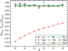 |
Fig. 6 Energy levels from the present Emu CI calculations for the nine lowest excited states compared to those from the NIST database (Kramida et al. 2019). |
Wavelengths (in Å) and line strengths (in au) for selected transitions of Fe XVIII compared with available data.
Lifetimes (in s) for the nine lowest excited states of F-like ions with Z = 20−30.
Static scalar and tensor dipole polarizabilities (in au) for the ten lowest levels of F-like ions with Z = 20−30.
4.2 Wavelengths and line strengths
The wavelengths and line strengths for some selected transitions of Fe XVIII are listed in Table 2 and are compared with the NIST values (Kramida et al. 2019) and earlier calculations (Si et al. 2016; Nandy & Sahoo 2014). For most of the transitions the agreement of our wavelengths and the NIST values is less than 0.3%, except that our results for 2s22p5 2 P3∕2 − 2s 2p6 2 S1∕2, 2s2 2p5 2 P3∕2 −  2 D5∕2, 2s2 2p5 2 P1∕2 − 2s 2p6 2 S1∕2, and 2s2 2p5 2 P3∕2 −
  2 D3∕2 transitions differ from the NIST values by about 1.5%. Apparently the present results and the MCDHF calculations from Si et al. (2016) show good agreement (within 5%) for all the tabulated E1, E2, and M1 transitions. The line strengths from Nandy & Sahoo (2014) are also consistent with other theories, but they exhibit a slightly larger difference for some E1 and M1 transitions, and are significantly lower for tabulated E2 transitions. Compared with experimental data, all the calculations for the E1 transitions underestimated the NIST values. For the
  2 D5∕2 − 2s2 2p5 2 P3∕2,
  2 P3∕2 − 2s2 2p5 2 P3∕2, and
  2 S1∕2 − 2s2 2p5 2 P1∕2 transitions the differences between theory and experiment are less than 5%; however, the differences for all other E1 transitions are about 20%, except for some very weak ones. On the other hand, the experimental information for the E2 and M1 transitions are very limited, and our results and the MCDHF calculations from Si et al. (2016) agree well with the NIST values for the 2s2 2p5 2 P1∕2 − 2s2 2p5 2 P3∕2 E2 and M1 transitions. The line strengths of electric-dipole, electric quadrupole, and magnetic dipole transitions for all the ions in which the ten lowest levels are involved are listed as a matrix in the tables available at the CDS. For brevity, comparisons of line strengths for other ions were not presented, but the situation is similar to the case of Fe XVIII. The available information can be obtained from the NIST database (Kramida et al. 2019) and in Si et al. (2016), Aggarwal (2019), and El-Sayed & Attia (2019).
4.3 Lifetimes and polarizabilities
A comparison of lifetimes for the nine lowest excited states of F-like ions with Z = 20−30 derived from our Emu CI calculations are displayed in Table 3 compared with other theoretical results (Si et al. 2016; Aggarwal 2019; El-Sayed & Attia 2019). As we discussed above, the uncertainties of the lifetimes listed in the table are given as 5%. One can easily find that the lifetime of any specific state decreases rapidly as the nuclear charge increases. The first excited state always has a much longer lifetime than other states, where our results show excellent agreement with the MCDHF calculations from Si et al. (2016), and the differences with Aggarwal (2019) and El-Sayed & Attia (2019) are also within 2%. For higher excited states, the lifetimes are very short and our results for most of these states are slightly longer. The discrepancies could be from the omission of magnetic-quadrupole (M2) transitions in our calculations.
An accurate determination of polarizabilities for some low-lying states of atoms and ions plays a central role in describing the interactions with an external electric field, and thus has wide applications in different areas. Table 4 lists the static scalar and tensor dipole polarizabilities for the ten lowest levels obtained by using the present line strengths. We did not find relevantworks for comparison; however, it is reasonable to assume an uncertainty of 3% from the uncertainties of our line strengths and energy levels. The polarizabilities for these ions (much smaller than neutral atoms) suggest that the strong Coulomb potentials make the influences of external fields weak, and that is why the proposal of using highly charged ions as candidates for optical clocks has recently become popular. It is worth noting that scalar polarizability of the second excited state is negative due to the large negative contributions from the first excited state and ground state. The 1s2core polarizabilities from Johnson et al. (1983) are also listed in Table 4, and have been added to the scalar dipole polarizabilities.
5 Summary
We presented large-scale relativistic B-spline configuration interaction calculations for F-like ions with Z = 20−30. For each ion, energy levels of the 250 lowest states relative to the ground state are reported and compared with available theoretical and experimental data. A large size of the CI space is adopted to take into account the majority of electronic correlations, while a numerical method called Emu CI is also considered to save computational resources with a loss of accuracy of less than 130 cm−1. The uncertainties of the results are estimated by detailed analysis, indicating that the total uncertainties on our transition energies are approximately 110, 1300, and 3800 cm−1 for the first, second, and higher excited states, respectively, most of which is the result of the setting of the 1s2frozen core. The obtained energy levels show a good agreement with the NIST data sets and with other theoretical and experimental values. The largest relative difference compared with the NIST values occurs at the second excited states, and the overall agreement is within 0.2o for most of the states. Setting the 1s2core electrons active would increase the level of accuracy significantly; however, the computation resource needed is tremendous and beyond our limit. This can only be done for some specific states that are strictly required for very accurate information. The line strengths of the E1, E2, and M1 transitions in which the ten lowest levels are involved; the electric scalar and tensor dipole polarizabilities of the ten lowest levels; and the lifetimes of the nine lowest excited states are also reported for all the ions. We believe that our extensive calculations could be useful in the modeling and diagnostics of line identifications or could make contributions to astrophysics and plasma communities.
Acknowledgements
We gratefully acknowledge the support from the National Natural Science Foundation of China No. 11974230, No. 11934004, and No. 11504094, and The Key Science Fund of Educational Department of Henan Province of China No.19A140013. We also would like to thank E.V. Kahl and J.C. Berengut, the authors of Ambit packages, for providing support and guidance in using their codes.
Appendix A Additional table
Energy levels (in cm−1) relative to theground state for the 250 lowest levels for F-like ions with Z = 20−30.
References
- Aggarwal, K. M. 2019, At. Data Nucl. Data Tables, 127-128, 22 [CrossRef] [Google Scholar]
- Berengut, J. C., Dzuba, V. A., & Flambaum, V. V. 2010, Phys. Rev. Lett., 105, 120801 [CrossRef] [PubMed] [Google Scholar]
- Berengut, J. C., Dzuba, V. A., Flambaum, V. V., & Ong, A. 2011, Phys. Rev. Lett., 106, 210802 [CrossRef] [PubMed] [Google Scholar]
- Berengut, J. C., Dzuba, V. A., Flambaum, V. V., & Ong, A. 2012, Phys. Rev. Lett., 109, 070802 [CrossRef] [PubMed] [Google Scholar]
- Bhatia, A. K., & Drachman, R. J. 1997, Phys. Rev. A, 55, 1842 [CrossRef] [Google Scholar]
- Bhatia, A. K., & Drachman, R. J. 1998, Phys. Rev. A, 58, 4470 [CrossRef] [Google Scholar]
- Bhatia, A. K., & Drachman, R. J. 1999, Phys. Rev. A, 60, 2848 [CrossRef] [Google Scholar]
- Clementson, J., & Beiersdorfer, P. 2013, ApJ, 763, 54 [NASA ADS] [CrossRef] [Google Scholar]
- Curdt, W., Landi, E., & Feldman, U. 2004, A&A, 427, 1045 [NASA ADS] [CrossRef] [EDP Sciences] [Google Scholar]
- Del Zanna, G., Dere, K. P., Young, P. R., Landi, E., & Mason, H. E. 2015, A&A, 582, A56 [NASA ADS] [CrossRef] [EDP Sciences] [Google Scholar]
- Derevianko, A., Dzuba, V. A., & Flambaum, V. V. 2012, Phys. Rev. Lett., 109, 180801 [CrossRef] [PubMed] [Google Scholar]
- Doschek, G. A., & Feldman, U. 2010, J. Phys. B At. Mol. Opt. Phys., 43, 232001 [NASA ADS] [CrossRef] [Google Scholar]
- Dzuba, V. A., Derevianko, A., & Flambaum, V. V. 2013, Phys. Rev. A, 87, 029906 [CrossRef] [Google Scholar]
- Dzuba, V. A., Flambaum, V. V., & Katori, H. 2015, Phys. Rev. A, 91, 022119 [CrossRef] [Google Scholar]
- El-Sayed, F., & Attia, S. M. 2019, Phys. Atom. Nucl., 82, 583 [CrossRef] [Google Scholar]
- Froese Fischer, C., & Tachiev, G. 2004, At. Data Nucl. Data Tables, 87, 1 [NASA ADS] [CrossRef] [Google Scholar]
- Geddes, A. J., Czapski, D. A., Kahl, E. V., & Berengut, J. C. 2018, Phys. Rev. A, 98, 042508 [CrossRef] [Google Scholar]
- Gu, M. 2005, At. Data Nucl. Data Tables, 89, 267 [NASA ADS] [CrossRef] [Google Scholar]
- Gu, M. F., Beiersdorfer, P., Brown, G. V., et al. 2007a, ApJ, 657, 1172 [NASA ADS] [CrossRef] [Google Scholar]
- Gu, M. F., Chen, H., Brown, G. V., Beiersdorfer, P., & Kahn, S. M. 2007b, ApJ, 670, 1504 [NASA ADS] [CrossRef] [Google Scholar]
- Hinnov, E., & Suckewer, S. 1980, Phys. Lett. A, 79, 298 [NASA ADS] [CrossRef] [Google Scholar]
- Johnson, W. R. 2007, Atomic Structure Theory (Berlin: Springer) [Google Scholar]
- Johnson, W. R., Kolb, D., & Huang, K. N. 1983, At. Data Nucl. Data Tables, 28, 333 [NASA ADS] [CrossRef] [Google Scholar]
- Jonauskas, V., Keenan, F. P., Foord, M. E., et al. 2004, A&A, 416, 383 [NASA ADS] [CrossRef] [EDP Sciences] [Google Scholar]
- Jönsson, P., Alkauskas, A., & Gaigalas, G. 2013, At. Data Nucl. Data Tables, 99, 431 [NASA ADS] [CrossRef] [Google Scholar]
- Kahl, E., & Berengut, J. 2019, Comput. Phys. Commun., 238, 232 [CrossRef] [Google Scholar]
- Kramida, A., Yu. Ralchenko, Reader, J., & NIST ASD Team 2019, NIST Atomic Spectra Database (ver. 5.7.1), [Online], available: https://physics.nist.gov/asd [2020, June 9]. National Institute of Standards and Technology, Gaithersburg, MD [Google Scholar]
- Landi, E., & Phillips, K. J. H. 2005, ApJS, 160, 286 [NASA ADS] [CrossRef] [Google Scholar]
- Li, J., Zhang, C., Si, R., Wang, K., & Chen, C. 2019, At. Data Nucl. Data Tables, 126, 158 [CrossRef] [Google Scholar]
- Nahar, S. N. 2006, A&A, 457, 721 [CrossRef] [EDP Sciences] [Google Scholar]
- Nandy, D. K., & Sahoo, B. K. 2014, A&A, 563, A25 [CrossRef] [EDP Sciences] [Google Scholar]
- Ouart, N. D., Safronova, A. S., Faenov, A. Y., et al. 2011, J. Phys. B, 44, 065602 [CrossRef] [Google Scholar]
- Podpaly, Y., Clementson, J., Beiersdorfer, P., et al. 2009, Phys. Rev. A, 80, 052504 [CrossRef] [Google Scholar]
- Reader, J. 1982, Phys. Rev. A, 26, 501 [CrossRef] [Google Scholar]
- Reader, J., Brown, C. M., Ekberg, J. O., et al. 1986, J. Opt. Soc. Am. B, 3, 1609 [CrossRef] [Google Scholar]
- Safronova, U. I., Namba, C., Murakami, I., Johnson, W. R., & Safronova, M. S. 2001, Phys. Rev. A, 64, 012507 [CrossRef] [Google Scholar]
- Safronova, A., Kantsyrev, V., Faenov, A., et al. 2012, High Energy Density Physics, 8, 190 [CrossRef] [Google Scholar]
- Safronova, M. S., Dzuba, V. A., Flambaum, V. V., et al. 2014a, Phys. Rev. Lett., 113, 030801 [CrossRef] [Google Scholar]
- Safronova, M. S., Dzuba, V. A., Flambaum, V. V., et al. 2014b, Phys. Rev. A, 90, 042513 [CrossRef] [Google Scholar]
- Shestov, S., Reva, A., & Kuzin, S. 2013, ApJ, 780, 15 [CrossRef] [Google Scholar]
- Si, R., Li, S., Guo, X. L., et al. 2016, ApJS, 227, 16 [CrossRef] [Google Scholar]
- Stadnik, Y. V., & Flambaum, V. V. 2014, Phys. Rev. Lett., 113, 151 301 [CrossRef] [PubMed] [Google Scholar]
- Sucher, J. 1980, Phys. Rev. A, 22, 348 [NASA ADS] [CrossRef] [MathSciNet] [Google Scholar]
- Träbert, E., Gwinner, G., Wolf, A., Tordoir, X., & Calamai, A. G. 1999a, Phys. Lett. A, 264, 311 [CrossRef] [Google Scholar]
- Träbert, E., Wolf, A., Linkemann, J., & Tordoir, X. 1999b, J. Phys. B, 32, 537 [CrossRef] [Google Scholar]
- Van Tilburg, K., Leefer, N., Bougas, L., & Budker, D. 2015, Phys. Rev. Lett., 115, 011802 [CrossRef] [Google Scholar]
- Warren, G. A., Keenan, F. P., Greer, C. J., et al. 1997, Sol. Phys., 171, 93 [CrossRef] [Google Scholar]
- Young, P. R., Dupree, A. K., Wood, B. E., et al. 2001, ApJ, 555, L121 [NASA ADS] [CrossRef] [Google Scholar]
- Zanna, G. D. 2006, A&A, 459, 307 [NASA ADS] [CrossRef] [EDP Sciences] [Google Scholar]
All Tables
Energy levels (in cm−1) relative to the ground state for the 250 lowest levels of Fe XVIII.
Wavelengths (in Å) and line strengths (in au) for selected transitions of Fe XVIII compared with available data.
Lifetimes (in s) for the nine lowest excited states of F-like ions with Z = 20−30.
Static scalar and tensor dipole polarizabilities (in au) for the ten lowest levels of F-like ions with Z = 20−30.
Energy levels (in cm−1) relative to theground state for the 250 lowest levels for F-like ions with Z = 20−30.
All Figures
|
Fig. 1 Schematic of the Emu CI approximation. The white part represents the terms neglected in this method. Effective CI matrix elements are shaded in gray. |
| In the text | |
|
Fig. 2 Convergence of the 12 lowest excited states when the CI basis set is increased from 7spdfg to 8spdfg. |
| In the text | |
|
Fig. 3 Comparison of the present Emu CI and full CI excitation energies for the 12 lowest excited states. |
| In the text | |
|
Fig. 4 Difference in percentage of energy levels from the present Emu CI calculations for the first excited state 2s2 2p52P1∕2 compared to those from NIST (Kramida et al. 2019) and other calculations (Si et al. 2016; Jönsson et al. 2013; Nandy & Sahoo 2014). |
| In the text | |
|
Fig. 5 Difference in percentage of energy levels from the present Emu CI calculations for the second excited state 2s 2p6 2 S1∕2 compared to those from NIST (Kramida et al. 2019) and other calculations (Si et al. 2016; Jönsson et al. 2013; Nandy & Sahoo 2014). |
| In the text | |
|
Fig. 6 Energy levels from the present Emu CI calculations for the nine lowest excited states compared to those from the NIST database (Kramida et al. 2019). |
| In the text | |
Current usage metrics show cumulative count of Article Views (full-text article views including HTML views, PDF and ePub downloads, according to the available data) and Abstracts Views on Vision4Press platform.
Data correspond to usage on the plateform after 2015. The current usage metrics is available 48-96 hours after online publication and is updated daily on week days.
Initial download of the metrics may take a while.