| Issue |
A&A
Volume 644, December 2020
|
|
|---|---|---|
| Article Number | A122 | |
| Number of page(s) | 20 | |
| Section | Interstellar and circumstellar matter | |
| DOI | https://doi.org/10.1051/0004-6361/202039149 | |
| Published online | 10 December 2020 | |
Polarisation properties of methanol masers
1
Department of Space, Earth and Environment, Chalmers University of Technology, Onsala Space Observatory,
Observatorievägen 90,
43992
Onsala,
Sweden
e-mail: This email address is being protected from spambots. You need JavaScript enabled to view it.
2
INAF – Osservatorio Astronomico di Cagliari,
Via della Scienza 5,
09047
Selargius,
Italy
Received:
10
August
2020
Accepted:
6
October
2020
Abstract
Context. Astronomical masers have been effective tools in the study of magnetic fields for years. Observations of the linear and circular polarisation of different maser species allow for the determination of magnetic field properties, such as morphology and strength. In particular, methanol can be used to probe different parts of protostars, such as accretion discs and outflows, since it produces one of the strongest and the most commonly observed masers in massive star-forming regions.
Aims. We investigate the polarisation properties of selected methanol maser transitions in light of newly calculated methanol Landé g-factors and in consideration of hyperfine components. We compare our results with previous observations and evaluate the effect of preferred hyperfine pumping and non-Zeeman effects.
Methods. We ran simulations using the radiative transfer code, CHAMP, for different magnetic field values, hyperfine components, and pumping efficiencies.
Results. We find a dependence between the linear polarisation fraction and the magnetic field strength as well as the hyperfine transitions. The circular polarisation fraction also shows a dependence on the hyperfine transitions. Preferred hyperfine pumping can explain some high levels of linear and circular polarisation and some of the peculiar features seen in the S-shape of observed V-profiles. By comparing a number of methanol maser observations taken from the literature with our simulations, we find that the observed methanol masers are not significantly affected by non-Zeeman effects related to the competition between stimulated emission rates and Zeeman rates, such as the rotation of the symmetry axis. We also consider the relevance of other non-Zeeman effects that are likely to be at work for modest saturation levels, such as the effect of magnetic field changes along the maser path and anisotropic resonant scattering.
Conclusions. Our models show that for methanol maser emission, both the linear and circular polarisation percentages depend on which hyperfine transition is masing and the degree to which it is being pumped. Since non-Zeeman effects become more relevant at high values of brightness temperatures, it is important to obtain good estimates of these quantities and the maser beaming angles. Better constraints on the brightness temperature will help improve our understanding of the extent to which non-Zeeman effects contribute to the observed polarisation percentages. In order to detect separate hyperfine components, an intrinsic thermal line width that is significantly smaller than the hyperfine separation is required.
Key words: masers / magnetic fields / stars: formation / stars: magnetic field / polarization
© ESO 2020
1 Introduction
The role of the magnetic field during star formation has been a topic of great debate for years. Many observations have been performed in the aim of detecting magnetic field morphology and strength towards star-forming regions. Several works have already demonstrated that astrophysical masers are powerful tools for investigating magnetic field properties in young protostars (recently reviewed by Crutcher & Kemball 2019, and references therein). Through the study of linearly and circularly polarised maser emission, it is possible to obtain information about the magnetic field, such as direction and strength, over spatial scales of 10–100 au (e.g. Vlemmings et al. 2010; Surcis et al. 2013). Moreover, different maser species and transitions probe different regions of the protostar, providing a unique picture of the physical conditions of the material where star-formation processes are ongoing (Surcis et al. 2011a). Masers can also help in investigating the link between the gas properties and the magnetic field: for instance, maser polarisation observations were used to infer a relationship between the density of the gas and the magnetic field acting in the region (Fish et al. 2006; Vlemmings 2008). Maser polarisation observations have also been used to infer the properties of the large-scale Galactic magnetic field (e.g. Green et al. 2012).
Circular polarisation has been detected in the majority of the maser species, such as hydroxyl, water, and methanol (Etoka et al. 2005; Vlemmings et al. 2006; Sarma et al. 2008; Surcis et al. 2011b; Caswell et al. 2011; Hunter et al. 2018). In particular, methanol masers have emerged as excellent tools for probing magnetic fields during star formation (e.g. Vlemmings 2008; Surcis et al. 2019; Momjian & Sarma 2019; Sarma & Momjian 2020, and references therein). Although the circularly polarised emission of methanol maser has been regularly detected, no exact estimates of the magnetic field strength have been possible due to the fact that the Landé g-factors were previously unknown (Vlemmings et al. 2011). Thanks to recent detailed calculations of the Landé g-factors for all methanol transitions and the associated hyperfine components (Lankhaar et al. 2016, 2018), it is now possible to obtain a complete interpretation of the methanol maser polarisation properties and infer the magnetic field characteristics.
In this paper, we investigate the methanol maser polarisation properties using the maser polarisation radiative transfer code, CHAMP (Lankhaar & Vlemmings 2019), performing several simulations of different methanol masers transitions, as described in Sect. 3. We report our results for the different masers transitions in Sect. 4, with a more detailed view on the one at 6.7 GHz given the large number of observations in the literature, along with a more general description of the most important features observed at other frequencies. Then, in Sect. 5, we compare the results of our simulations with previous observations and we discuss the importance of hyperfine preferred pumping, its effect on the polarisation fraction and the V spectra, and the presence of non-Zeemaneffects. In Sect. 6, we present our conclusions and future perspectives, considering this work asa potential starting point for a larger and more detailed study of magnetic fields based on the fact that further high-resolution observations will help improve our understanding of the action of preferred hyperfine pumping.
2 Origin of circular polarisation and non-Zeeman effects
One of the major sources of the circular polarisation of molecular lines is the Zeeman effect (Zeeman 1897; Fiebig & Guesten 1989; Sarma et al. 2001). According to the theory, under the action of a magnetic field B, the emission from a molecule is separated into several components due to the magnetic sub-levels. The shift between these components is named Zeeman splitting and it can be used to derive the amount of circular polarisation, which is proportional to the magnetic field strength. Studying circular polarisation in maser emission is, therefore, fundamental for inferring the magnetic field strength of the masing region.
In general, the saturation level and the nature of the masing molecule (paramagnetic or non-paramagnetic) are the main factors responsible for the maser polarisation properties (e.g. Watson 2008; Dinh-v-Trung 2009). In addition,maser polarisation is also affected by the ratio between the Zeeman frequency, gΩ, the rate of stimulated emission, R, and the decay rate of the molecular state Γ (Western & Watson 1984).
The rate of stimulated emission can be obtained from
 (1)
(1)
where A is the Einstein coefficient which depends on the hyperfine transition, k and h are the Boltzmann and Planck constants, respectively, and ν is the maser frequency; TB and ΔΩ are the maser brightness temperature and beaming solid angle (see also Vlemmings et al. 2011).
The Zeeman frequency is defined as
 (2)
(2)
where B is the magnetic field in G, ℏ is the reduced Planck constant, and g is the Landé g-factor (see e.g. Nedoluha & Watson 1990a). In case of a paramagnetic molecule (e.g. OH), μ is the Bohr magneton (μB = eℏ∕2mec), whereas in the case of a non-paramagnetic molecule (e.g. H2O or CH3OH) it is the nuclear magneton (μN = eℏ∕2mnc), where e is the electron charge, and me and mn are the electron and nucleon mass, respectively.
The magnitude of the Zeeman effect depends on gΩ and it is different between paramagnetic and non-paramagnetic molecules. Since μB ∕μN ~ 103, paramagnetic molecules can show a split that is three orders of magnitude larger than the non-paramagnetic ones (Vlemmings 2007). Moreover, for paramagnetic molecules, the Zeeman frequency gΩ is usually larger than the intrinsic line width; thus, the Zeeman components are separated and resolved and from the Zeeman splitting. So, it is possible to obtain the magnetic field along the line of sight without ambiguity, B∥ = Bcosθ, with θ defined as the angle between the magnetic field and the line of sight. On the contrary, for non-paramagnetic molecules such as methanol, gΩ is smaller thanthe line width and the Zeeman components overlap. In this case, it is more complicated to infer circular polarisation measurements because it also depends on the saturation level and non-Zeeman effects might come about, compromising the measurement of the regular Zeeman splitting. A maser is defined saturated when the rate of stimulated emission R exceeds the decay rate of the involved molecular state Γ.
2.1 Rotation of the symmetry axis
When gΩ > R, the magnetic field direction is the quantisation axis, but when the maser brightness increases or there is weak B, then R can become much larger than gΩ and a rotation of the symmetry axis can occur. This change in the quantisation axis can generate an intensity-dependent circular polarisation similar to the regular Zeeman splitting (Nedoluha & Watson 1990b). Therefore, it is important to know when this effect might occur and we can do so by estimating R and gΩ. The ratio between the Zeeman splitting rate and the stimulated emission rate is
![Mathematical equation: \begin{equation*} \frac{R}{g\Omega}\simeq 1.7{{1}\over{g}} {{[\textrm{mG}]}\over{B}} {{T_b}\over{[10^{10}\,\textrm{K}]}}{{\Delta\Omega}\over{[10^{-2}\,\textrm{sr}]}} {{[\textrm{GHz}]}\over{\nu}} {{A}\over{[10^{-7}\textrm{s}^{-1}]}}. \end{equation*}](/articles/aa/full_html/2020/12/aa39149-20/aa39149-20-eq3.png) (3)
(3)
The rotation of the symmetry axis might occur when  . In the case of the 6.7 GHz methanol maser, considering the typical values for the beaming solid angle ΔΩ = 10−2 K sr, a magnetic field B = 10 mG, A = 1.074 × 10⁻⁹ s−1 and an average Landé factor calculated using all hyperfine components, ga = 0.236 (Lankhaar et al. 2016), this effect might come about only when the maser is deeply saturated, with TB ≥ 1012 K. This result also holds when considering the largest and the smallest g-factor of the 6.7 GHz methanol maser hyperfine transition 3 → 4A and 5 → 6B, respectively, leading to TB ≥ 1010 K.
2.2 Effect of magnetic field changes
There are also other non-Zeeman mechanisms that can generate high levels of polarisation at lower TB. One of these effects is due to magnetic field changes along the maser path, for example, a rotation (Wiebe & Watson 1998). This rotation converts the linear polarisation fraction, PL to a circular polarisation fraction, PV. Considering a rotation of 1 rad in the magnetic field direction along the maser path, the fractional circular polarisation generated by this mechanism is  . According to previous observations of 6.7 GHz methanol masers, this mechanism only produces minor contributions (Vlemmings et al. 2011). For example, the polarisation observed in high angular resolution observations for 6.7 GHz masers ranges usually from 1 to 4%. Therefore, the change of magnetic field direction along the maser propagation direction can contribute at most ~ 0.04%, that is only a fraction of the observed values of PV (e.g. Surcis et al. 2009, 2012, 2019). However, this effect can be important for very high levels of linear polarisation PL ~ 10%, causing an extra PV ~ 0.25%. Recent methanol maser observations by Breen et al. (2019) have registered a level of linear polarisation of ~ 7.5%, which we discuss in Sect. 5.
2.3 Anisotropic resonant scattering
Resonant scattering is a higher order radiation matter interaction that describes the absorption and subsequent immediate emission of a photon by a molecule or atom. Houde et al. (2013) point out that forward resonant scattering is coherent in nature and that a large ensemble of molecules collectively scatter incoming radiation. In the presence of a magnetic field, such collective resonant scattering leads to a significant phase shift between the left and right-circularly polarised radiation modes. This process is called anisotropic resonant scattering (ARS) and leads to the conversion of linear polarisation (by way of the Stokes U component) to circular polarisation.
Houde (2014) propose that the circular polarisation of SiO masers might be generated through the anisotropic resonant scattering of linearly polarised maser radiation by a foreground cloud between the maser and the observer. The foreground cloud may be out of the velocity range of the maser. Alternatively, the collective resonant scattering of radiation might be a feature of the radiative transfer of maser radiation. Overall, CHAMP only accounts for first-order radiative interactions and neglects resonant scattering. Proper estimates of the probability of ARS in relation to maser amplification have to be developed before the importance of ARS to maser radiative transfer can be evaluated.
Circular polarisation profiles generated through ARS do not necessarily lead to the antisymmetric S-shaped profile that characterises Zeeman circular polarisation. Antisymmetric Stokes-V profiles cab be generated by ARS only under special conditions. The Stokes-V profiles of methanol masers are generally characterised by an antisymmetric spectrum.
2.4 Other non-Zeeman effects
Other non-Zeeman effects could be attributed to instrumental effects and the presence of a velocity gradient across an extended source. Potential instrumental effects causing extra circular polarisation depend on the instrument characteristics and these are generally reported in the literature. A velocity gradient could generate an S-shaped V spectrum like the one produced by the Zeeman effect, but this effect is rare with masers since they are point-like sources producing narrow spectral lines developing in a narrow velocity range (e.g. Sarma & Momjian 2020).
3 Methods
To investigate the polarisation of methanol masers by a magnetic field and its effects on the hyperfine structure, we ran simulations using the CHAMP code (Lankhaar & Vlemmings 2019). CHAMP is a maser polarisation radiative transfer code that takes into account all dominant hyperfine components of a molecule and their individual Landé factors. CHAMP implements both the methods in Nedoluha & Watson (1992, hereafter N&W92), which do not treat non-Zeeman effects, and those in Nedoluha & Watson (1994, hereafter N&W94), which do consider non-Zeeman effects. The user can choose either of the two methods. In addition to a combined treatment of all hyperfines according to their transition probabilities, CHAMP includes the possibility of (i) changing the pumping efficiency for different hyperfine components, and (ii) anisotropic pumping.
The linear polarisation degree is defined as
 (4)
(4)
the polarisation angle is
 (5)
(5)
and the circular polarisation degree is
 (6)
(6)
where I, Q, U, and V are the Stokes parameters.
The polarisation angle is relative to the projection of the magnetic field direction onto the plane of the sky, which we take to be north-south (unless along the maser beam when θ = 0°).
In Table1, we report the maser transitions that we used in our simulations. Since the size of the masing region or the maser beaming angle ΔΩ are often unknown, for comparison with our models, we give the value of the brightness temperature, TB, assuming a maser spot size of 3 mas. We also give a lower limit for TB, based on the observations from Breen et al. (2019), Sarma & Momjian (2020), Momjian & Sarma (2019), Surcis et al. (2009, 2019). In the case of the 12.2 GHz maser, we did not model a specific source but we give a typical value on the basis of the previous work by Moscadelli et al. (2003). For known spectral features, TB can be derived using the equation
![Mathematical equation: \begin{equation*} \frac{ T_{\textrm{B}}}{[\mathrm{K}]} = \frac{S(\nu)}{[\mathrm{Jy}]}\left(\frac{\Sigma^2}{[\mathrm{mas}^2]}\right)^{-1}\zeta_{\nu},\end{equation*}](/articles/aa/full_html/2020/12/aa39149-20/aa39149-20-eq9.png) (7)
(7)
where S(ν) is the detected flux density, Σ is the maser angular size, and ζν is a constant that includes a proportionality factor obtained for a Gaussian shape (Burns et al. 1979) and which scales with the frequency according to the relation:
![Mathematical equation: \begin{equation*} \zeta_{\nu}\simeq 6.1305\times10^{11}\left(\frac{\nu}{[\mathrm{GHz}]}\right)^{-2}\frac{\mathrm{mas^2}}{\mathrm{Jy}}\mathrm{K}.\end{equation*}](/articles/aa/full_html/2020/12/aa39149-20/aa39149-20-eq10.png) (8)
(8)
In Table 1, we also report the method we used between N&W92 and N&W94. We performed simulations for different methanol maser transitions at different magnetic field strengths, angular momentum transitions, and propagation angles θ. The molecular parameters used in the simulation are presented in Tables A.1–A.13 and taken from Lankhaar et al. (2018) or, for the newly discovered transitions observed by Breen et al. (2019), they have been computed for this purposes of this paper. In these tables, the quantities marked as “g-factors” are defined as μN g∕ℏ. We ran calculations assuming an intrinsic thermal velocity width vth = 1 km s−1. For all the transitions, we used a pumping efficiency of δ = 0.02, a decay rate of the upper and lower level of Γ = 1 s−1 (Vlemmings et al. 2010; Lankhaar & Vlemmings 2019), and in the case of anisotropic pumping, the anisotropy degree, ɛ = 0.01. The parameters are described in Lankhaar & Vlemmings 2019.
4 Results
4.1 6.7 GHz methanol maser
We report on our simulations of the 6.7 GHz methanol maser across a range of different magnetic field strengths (1, 3, 10, 20, 30, and 100 mG), with varying luminosity and magnetic field angles. The results of these simulations are shown in several figures in the body of the paper (Figs. 1–3) and in the appendix (Figs. A.1– A.15). The magnetic field strength, the thermal velocity width vth, the propagation angle θ, and the transition angular momenta are indicated in each figure. In Figs. 1–3, A.1, and A.6–A.11, the panel at the top-left that is labelled “baseline” indicates a maser emission where all the eight hyperfine transitions contribute equally, while all other panels assume a preferred pumping for the indicated i → j transition. The preferred pumping rate is ten times larger than the other transitions’ rate.
We present, in Fig. 1, the linear and circular polarisation fraction, PL and PV, as a function of the maser luminosity for five different θ values. With a vertical line, we mark the locus gΩ = 10R, which for the 6.7 GHz methanol maser, falls at TBΔΩ ~ 1010 K sr. For TBΔΩ ≲ 1010 K sr, the Zeeman frequency gΩ is much higher than the stimulated emission rate R. On the contrary for TBΔΩ ≳ 1010 K sr, the Zeeman frequency is similar to or lower than the rate of stimulated emission. As already mentioned in Sect. 2, masers can be affected by several non-Zeeman processes that can either intensify or generate linear and circular polarisation. Typically, gΩ = 10R has been used in the literature (e.g. by Pérez-Sánchez & Vlemmings 2013) to mark the region where non-Zeeman effects become relevant and, therefore, inferring magnetic field properties becomes more challenging since the magnetic field is not directly related to PL and PV. One of the most prominent non-Zeeman effects is the rotation of the symmetry axis that can occur when gΩ < 10R (Pérez-Sánchez & Vlemmings 2013; Wiebe & Watson 1998), thus, we decided to indicate gΩ = 10R as an upper limit for maintaining a reliable level of PL and PV.
A clear dependence on the hyperfine transitions is shown by PL and PV as well as on the magnetic field strength and on the angle θ. From these plots, it is quite evident that each single hyperfine component is affected by the magnetic field in a different way and, therefore, in the presence of preferred hyperfine pumping, we observe a particular level of the polarisation fraction. At a first glance, these dependences appear most prominent above TB ΔΩ, corresponding to gΩ = 10R, however, noticeable effects also occur when gΩ > 10R for several transitions, such as 3 → 4 A and 4 → 5 A. For example, the dependence on θ shown in Fig. A.5 is different from the usual cosθ dependence (Watson & Wyld 2001), also for TBΔΩ below gΩ = 10R. In addition, these dependences seem weaker for PV compared to the case of PL, unless the magnetic field is very high, namely, ~100 mG (Fig. A.1), or the hyperfine is preferentially pumped by a large degree, that is, ~ 100 times (Fig. A.3).
We now consider the PL and PV values at gΩ = 10R. When θ = 90° and B = 10 mG, the maximum linear polarisation fraction is found to be on the order of 3% for the hyperfine transition 4 → 5 A. When θ = 0° and B = 10 mG, we obtain a maximum circular polarisation fraction on the order of 1% for the hyperfine transition 3 → 4 A. As the magnetic field strength increases, the position of gΩ = 10R falls at a higher TBΔΩ. Thus, for B = 100 mG, PL can reach 10% in the hyperfine transitions 4 → 5 A at θ = 90o, while PV can rise up to 8% when the hyperfine transition 3 → 4 A is preferentially pumped and θ = 0o.
We also investigated different degrees of preferred pumping for the two strongest hyperfine transitions 3 →4 A and 4 →5 A. We observed that both the linear and circular polarisation fractions increase with the preferred pumping. These results are shown in Figs. A.3 and A.4, where the linear and circular polarisation fractions are plotted as a function of the maser luminosity. Different degrees of preferred pumping are shown in different colours for the two hyperfine transitions, assuming a magnetic field of 10 mG. The vertical dotted lines indicate when gΩ = 10R.
In Tables 2 and 3, we report the PL and PV values taken at gΩ = 10R, for all the masers and for a magnetic field, B = 10 mG. The results of the simulation performed with other magnetic field strengths (1 and 100 mG) are given in Fig. A.1.
In Fig. 2, from top to bottom, respectively, we plot the linear polarisation fraction PL, the circular polarisation fraction PV, and the linear polarisation angle ψ as a function of the propagation angle θ and of the rate of stimulated emission for a magnetic field of 10 mG. These plots are symmetric along the line θ = 90°. The results of the simulation performed with other magnetic field strengths are given in Figs. A.6–A.8.
Also in this case, PL shows a dependence on the magnetic field strength and on preferred hyperfine pumping. Also, PL presents a sharp drop around the Van Vleck angle θ = 54°. It peaks around θ = 90° and log(R∕gΩ) = 1 (the peak ismarked with a star in Fig. 2, top), with a secondary peak around θ = 30° and log (R∕gΩ) = 2. This morphology is consistent across different magnetic field strengths and angular momenta of the transitions. We observe that also PV contours show a dependence on magnetic field strength and hyperfine transitions (Fig. 2, middle).The contour morphology shows two peaks (plus their symmetric counterparts at θ > 90°) located approximately at log(R∕gΩ) ~ 2.5 and θ ~ 50°, and at log(R∕gΩ) ~−2 and θ ~ 0°. The first one is dominant atlower B strengths (1, 3, 10 mG), while the second becomes more important at higher B (20, 30, 100 mG). As theB strength increases, some hyperfine transitions present emerging features in the ψ contours, where the polarisation angles flip. For instance, in the case of B = 10 mG (Fig. 2, bottom), the transition 5 →6 B presents two emergingregions located at log(R∕gΩ) ~ 0.5 and θ ~ 25°. Similar marks appear also for magnetic fields of 30 and 100 mG in the hyperfine transition 3 →4 A. We notice a 90° flip of the polarisation angle ψ happening around the Van Vleck angle and this trait becomes sharper with increasing magnetic field strength. This characteristic has been observed also for SiO and H2O masers (Vlemmings et al. 2006; Tobin et al. 2019). Generally, when the saturation level is low (log (R∕gΩ) < 0), the linear polarisation angle ψ appears quite stable in the range of 0° < θ < 54°, while variations of 20°–40° are visible for high levels of saturation. Around θ ~ 90°, ψ ~ 90° for almost all the saturation values. In these plots, we do not take the limit gΩ = 10R into account and, therefore, the strongest peak in PL ~ 0.2 and PV ~ 0.02, registered for the hyperfine transition 3 →4 A, are due to non-Zeeman effects.
In Fig. 3, the linear and circular polarisation fraction and the polarisation angle are plotted as functions of the propagation angle θ for different brightness temperatures in a magnetic field B = 10 mG. From Fig. 1, we know that for the 6.7 GHz methanol maser gΩ = 10R happens around TBΔΩ ~ 1010 K sr. When TBΔΩ > 1010 K sr and gΩ ≪ 10R, the maser starts to saturate and some non-Zeeman effects (such as the rotation of the symmetry axis) can come about. At that point, PL decreases when approaching the Van Vleck angle from both smaller and greater angles, and at the Van Vleck angle, PL has a minimum. This behaviour is maintained across different levels of saturation. We note that PL reaches its highest values when θ is greater than Van Vleck angle and for TBΔΩ ~ 1012−1013 K sr.
Looking at the circular polarisation profile, when TBΔΩ < 1010 K sr, the maser is not saturated and PV decreases for increasing θ, following the cosine profile described by Watson & Wyld (2001). In this regime, PV can be directly related to the magnetic field strength. When the maser saturates and TB ΔΩ > 1010 K sr, a rotation of the symmetry axis might come about, and PV is no longer linked to magnetic field strength. In Fig. A.5, we plot the cosine (dotted line) for different TB ΔΩ (solid line) to show this behaviour. We also observe an inversion of the linear polarisation angle corresponding to the Van Vleck angle, which is sharp for TBΔΩ < 1010 K sr and it becomes smoother with increasing brightness temperatures.
We also produced spectra of the 6.7 GHz methanol maser for different levels of saturation. We observe that the line broadens as the maser starts to saturate. Also the Stokes Q, U, and V intensify for high saturation levels. It is also interesting to observe that when preferred pumping is acting, a flip of the S-shape profile of the circular polarisation can be observed between different hyperfine transitions. The S-shaped Stokes V profile in Fig. A.13 for the 3 →4 A transition has the same shape as it does the baseline profile in Fig. A.12, but the profile reverses for the 8 →7 A transition in Fig. A.14. All Stokes parameters are plotted and several propagation angles θ are taken into account, assuming a magnetic field of 10 mG and v=1 km s−1.
In addition, we investigated anisotropic pumping and found, as already noted for SiO masers (Lankhaar & Vlemmings 2019), an increase of linear polarisation fraction up to 100%. In light of methanol maser pumping, the amount of anisotropy that can occur is low and since such a high level of linear polarisation has never been observed, we expect that anisotropic pumping can be considered less important for methanol masers than for SiO masers. Anisotropic pumping in SiO masers occurs primarily through the absorption of IR radiation from a nearby central stellar object. Methanol masers are either pumped collisionally (class I) or radiatively (class II). Collisional pumping generally does not introduce any anisotropy in the molecular states. The radiative pumping of class II masers can be anisotropic, albeit less so than compared to the case of SiO masers, since it occurs through co-spatial dust. Additionally, the high density of class II masers de-polarises the molecular states (Lankhaar & Vlemmings 2020), resulting in generally low degrees of anisotropic pumping. We also investigated the effect of an amplification of background polarised emission and we find that it does not contribute significantly to the linear polarisation fraction unless that background emission itself is already polarised at a high-enough level.
Methanol maser transitions considered in our simulations and observational parameters.
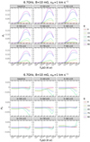 |
Fig. 1 6.7 GHz methanol maser linear and circular polarisation fraction as a function of the maser luminosity for five different θ. The vertical line marks TBΔΩ where gΩ = 10R. The magnetic field strength is 10 mG, the thermal velocity width is 1 km s−1, and the preferred hyperfine transitions are indicated in each panel. The panel at the top left labelled “baseline” indicates a fixed pumping rate equal for all the hyperfine transitions, while all others assume a 10 × preferred pumping for the indicated i → j transition. The results of the simulation performed with other magnetic field strengths are given in Appendix A. |
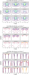 |
Fig. 2 6.7 GHz methanol maser linear polarisation fraction PL (top), circular polarisation fraction PV (middle), and linear polarisation angle ψ (bottom) plotted as a function of the propagation angle θ and the rate of stimulated emission. Stars indicate the position of the peak of PL. Magnetic field strength is 10 mG, thermal velocity width is 1 km s−1 and the hyperfine transitions are indicated in each panel. The panel at the top-left labelled “baseline” indicates a fixed pumping rate equal for all the hyperfine transitions, while all others assume a 10 × preferred pumping for the indicated i → j transition. The results of the simulation performed with other magnetic field strengths are given in Appendix A. |
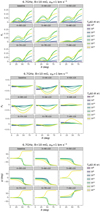 |
Fig. 3 6.7 GHz methanol maser linear polarisation fraction PL (top), circular polarisation fraction PV (middle) and polarisation angle ψ (bottom) plotted as a function of the propagation angle θ for different brightness temperatures. Panels as in Fig. 2. |
PL upper limits at gΩ = 10R, for B = 10 mG.
PV upper limits at gΩ = 10R, for B = 10 mG.
4.2 Other methanol maser transitions
For the other methanol maser transitions, we investigated PL and PV as a function of the maser luminosity for five different θ values and magnetic fields of 10, 20, and 30 mG. In the case of 25 GHz methanol maser, we also investigated a magnetic field of 100 mG. All the well-known maser transitions are modelled using the N&W94 code that can treat non-Zeeman effects (see Table 1), and only the lesser known transitions, such as 6.2, 7.7, 7.8, 20.3, 20.9, 37.7, and 46 GHz, have been investigated with the N&W92 code. The N&W92 code is not capable of dealing with non-Zeeman effects and, therefore, the simulations stop at gΩ = 10R. Within this limit, they behave like the other masers modelled with the N&W94 code.
In general, also at these other frequencies, PL and PV show a dependence on the hyperfine transitions, on the magnetic field strength, and on the angle θ, although less so for PV compared to PL unless the magnetic field is very high (~100 mG) or a hyperfine is preferentially pumped by a large degree (~100 times), consistent with our results for 6.7 GHz masers reported in Sect. 4.1. We confirm also for these transitions that hyperfinepreferred pumping can influence the polarisation fraction. In Tables 2 and 3, we report PL and PV for these maser transition, in case of B = 10 mG and taken at gΩ = 10R. Usually the maximum value of PL and PV is reached for θ = 90° and θ = 0°, respectively. In the case of the 25GHz maser, the maximum in PV is registered for the hyperfines 4 →4 A and B and 6 →6 B, that are the transitions where the g-factors are highest. The plots with the results of the simulations for the 6.2 GHz baseline in a magnetic field B = 10 mG are given in Fig. A.2.
Contour plots were produced only for simulations made with the N&W94 code. The 12, 25, 36, 44, and 45 GHz masers show contours similar to the 6.7 GHz. PL and PV typically present the same morphology reported for the 6.7 GHz with a dependence on the magnetic field strength and hyperfine transitions. The PL peaks are located in the same positions registered for the 6.7 GHz, around θ = 90° and log (R∕gΩ) = 1 around θ = 30° and log (R∕gΩ) = 2. The PV peaks are situated approximately at log(R∕gΩ) ~ 2.5 and θ ~ 50°, and at log(R∕gΩ) ~−2 and θ ~ 0°. Also for these masers, the peaks become more evident as the magnetic field strength increases. The polarisation angle shows a flip of 90° around the Van Vleck angle. Generally, ψ presents a region of stability in a range 0° < θ < 54° around − 2< log(R∕gΩ) < 0. This region in the 25 GHz maser is limited only to the area around log(R∕gΩ) ~−2.
Additionally, for these transitions, we observe high levels of PL and PV due to non-Zeeman effects. When the maser is not saturated, PV decreases for increasing θ, as predicted by Watson & Wyld (2001), whereas for saturated masers, the curves do not follow the cosines. We show this effect in Fig. A.5 for the baselines of the 6.2, 6.7, 25 and 45 GHz masers. In the case of the 6.2 GHz maser, we report the values until R∕gΩ = 10 and we see that all TB are following the cosine curve and non-Zeeman effects are not present. On the contrary, for the three other masers, we can see that the PV curves for high brightness temperatures and high levels of saturation do not decrease with increasing θ. Instead, they peak and show non-Zeeman effects that can lead to an overestimation of the magnetic field.
In these masers, we also identify an inversion of the linear polarisation angle close to the Van Vleck angle, which is sharp when the masers start to saturate and then becomes smoother with increasing brightness temperatures.
Looking at the circular polarisation fraction of 25, 36, 44, and 45 GHz, we can see that they appear stable also for TB ΔΩ above R∕gΩ = 10. As an example, in the case of the 25 GHz maser, we obtain at R∕gΩ = 10 a TBΔΩ ~ 109K sr for B = 10 mG. Here, PL starts to increase while PV keeps its stability until TB ΔΩ ~ 1010 K sr. Therefore, it might be that for PV, non-Zeeman effects become dominant only for TB higher than those where PL is sensible. However, from Fig A.5, the 25 GHz maser already presents, at TB ΔΩ ~ 1010 K sr, a curve that slightly deviates from the cosine, indicating that some non-Zeeman effects are already at work. For the other masers. we observe similar deviations.
4.3 6.2 GHz methanol maser
Of the masers studied here, the 6.2 GHz maser recently discovered by Breen et al. (2019) presents the largest hyperfine split of ~ 1 km s−1. The two peaks appear quite similar in intensity. To investigate the two hyperfine components, we ran the models for thermal line widths vth = 1, 1.25, and 1.50 km s−1 and we givethe results of the simulations in Fig. A.15. We see that for vth =1 km s−1, the two components are separated and they start to blend for vth =1.25 km s−1. At vth =1.5 km s−1, the two hyperfines appear totally blended in one single line.
This case illustrates why it is complicated to detect different hyperfine components of methanol masers at other frequencies. An intrinsic thermal line width that is less that the hyperfine split (vth <1.25 km s−1 in this case)is necessary to observe the hyperfine components; otherwise we can only detect one single blended component. However, when the split is large enough with respect to the intrinsic thermal line width, our simulations predict that multiple components can be observed.
5 Discussion
5.1 Comparison between models and observations
Within the limit gΩ = 10R, our model predicts linear and circular polarisation fractions that can be considered the upper limits and any polarisation above them are likely to include some non-Zeeman contributions. We compared the PL and PV observed in methanol masers (Table 1) with the results of our simulations (Tables 2 and 3for B = 10 mG). Overall, we noted that linear polarisation fraction predictions are mostly lower than the observed values, even for magnetic fields higher than 10 mG, while in the case of circular polarisation fractions, we often observe predictions higher than the observed values. In the following, we discuss each transition, comparing the observations and models and taking into account brightness temperatures, magnetic fields, and the presence of non-Zeeman effects.
5.1.1 6.7 GHz methanol masers
We compared the results of our simulations with 6.7 GHz maser observations from Breen et al. (2019), and Surcis et al. (2019, 2009); these masers are reported in Table 1. These works reported high PL on the order of 7.5, 8.1, and 4.5% respectively. We selected some extreme measurements of PL from the works of Surcis et al. and 6.7 GHz methanol masers typically present lower values, ranging from 1 to 4% (Surcis et al. 2019, and references therein).
We now discuss the possible action of non-Zeeman effects on the three selected 6.7 GHz methanol masers and reported in Table 1. The observed brightness temperatures range between 1011 –1013 K and, assuming ΔΩ ~ 10−2 sr, the TBΔΩ obtained from observations vary between 109 and 1011 K sr. Our 6.7 GHz methanol maser model gives TBΔΩ ~ 1010 K sr at gΩ = 10R, for a magnetic field of 10 mG, but when the magnetic field strength reaches B = 100 mG, the limit increases by one order of magnitude becoming TBΔΩ ~ 1011 K sr. This indicates that the selected masers are not affected by the rotation of the symmetry axis, but might be influenced by other non-Zeeman contributions (e.g. a rotating magnetic field along the maser direction) that can occur even at a modest TB. Thus, if we consider gΩ = 10R as an upper limit, we can estimate that the maximum brightness temperature that is reachable before being severely affected by non-Zeeman effects is ~1012 K (for B = 10 mG) or ~ 1013 K (for B = 100 mG).
For the 6.7 GHz maser transition observed by Breen et al. (2019), we do not have information regarding the magnetic field strength, but TB inferred from observations is within thelimit gΩ = 10R for both B = 10 mG and B = 100 mG. According to our model, such a high level of PL can be generated by a high B or by a specific hyperfine preferred pumping or by a combination of both. Indeed for B = 100 mG, it is possible to reach a PL ~ 10% (see Fig. A.1, e.g. with the transitions 4 → 5A and B). In addition, under the action of different preferred pumping, from 3 to 100 times over the baseline level, the linear and circular polarisation fractions increase and can reach, depending on the angle, up to 7.5%, even in B = 10 mG (see Figs. A.3 and A.4). Breen et al. (2019) also reported a PV = 0.5%, which is within the values reported by our model for a B = 10 mG (Table 3). However PrmV = 0.5% is also consistent with the results of our model considering a B = 100 mG and an hyperfine preferred pumping on the transition 4 → 5A. In any case, given the high PL observed, we cannot exclude the influence of some non-Zeeman effects. Since the TB inferred from observations is within the gΩ = 10R limit, we can rule out the rotation of the symmetry axis, but it could be possible to see a contribution in PV of ~ 0.14% due to magnetic field changes along the maser path (as described in Sect. 2.2).
Surcis et al. (2019) reported B > 182 mG, PL = 8.1% and PV = 2.1% for the maser feature WH3(OH).22 and the TB inferred from their observations is ~1013 K. These values are in agreement with our models for a magnetic field B = 100 mG and within the gΩ = 10R limit. However, since the PL is high, we cannot exclude minor non-Zeeman contributions affecting PV that could amount to ~0.16% due to magnetic field changes along the maser path (Sect. 2.2).
In the case of W75N, Surcis et al. (2009) estimated a TB ΔΩ < 109 K sr and based on ΔΩ ~ 10−1 sr and a maser angular size of 7 mas, they obtained θ = 70° and B = 50 mG. They also registered a PL = 4.5% and a PV = 0.2%. As for W3(OH), this value of PL and PV can be generated under the action of different degrees of hyperfine preferred pumping and B = 10–100 mG. If we exclude a different pointing direction of the magnetic field, hyperfine preferred pumping could be probable in the case of W75N: indeed, if we compare the S-shape profile of the observed V spectrum with the synthetic one, we see that the emission detected by Surcis et al. (2009) is compatible with a preferred pumping on hyperfine transitions 7 →8A, or 6 →7A. We note that these are not the same hyperfines of Tables 2 and 3.
5.1.2 25 GHz methanol masers
Sarma & Momjian (2020) observed 25 GHz methanol masers in two different epochs in the OMC–1 region. They reported for the two detections a level of PV ~ 0.3% and PV ~ 0.4% and, based on the low TBΔΩ, conclude that non-Zeeman effect likely contributes little to this percentage. From our models, in the case of B = 100 mG and with TBΔΩ ~ 106 K sr, we confirm that the non-Zeeman effects are neglegible and we found a PV ~ 1%, for the strongest hyperfine transitions, which has also been considered by Sarma & Momjian (2020). While this value is still higher than the measured values, we note that our simulations were run for vth = 1 km s−1. At TBΔΩ ~ 106 K sr, our spectra have a full width at half maximum (FWHM) line-width of slightly less than half that of the observed spectrum (0.24 km s−1 vs. 0.53 km s−1). Since in the normal Zeeman interpretation, the fractional polarisation is inversely proportional to the line-width this indicates that the observed polarisation in OMC-1 may indeed be the result of a magnetic field of ~100 mG.
From our models, in the case of B = 30 mG, we derive at the gΩ = 10R limit a value of TBΔΩ ~ 109 K sr and PV ~ 0.2% for the same hyperfine transitions considered by Sarma & Momjian (2020). While this indicates that a level of circular polarisation can be reached that is similar to the observed level for a smaller magnetic field strength, this only occurs for values of TB ΔΩ that are more than three orders of magnitude larger than estimated from the observations. In that case, part of PV originates from non-Zeeman effects, which do not contribute at the lower observed TB ΔΩ. Alternatively, if the maser spot size is overestimated and, thus, the TB is underestimated, and ΔΩ is significantly higher, non-Zeeman effects might, after all, be present in the observed signal. Currently, however, there are no observational indications that either case is the valid one, leading us to conclude that the normal Zeeman analysis performed in Sarma & Momjian (2020) can be used and that the 25 GHz methanol masers trace a shock-enhanced magnetic field.
5.1.3 36 GHz methanol masers
Sarma & Momjian (2009) detected 36 GHz methanol masers across the M8E region with PV ~ 0.1% and an estimated magnetic field of BLOS ~ 20–30 mG. Also, Breen et al. (2019) reported a very low level in both linear and circular polarisation fractions, specifically, lower than 0.5%. From our simulations, we can confirm a low PV for this maser and we find an agreement with the observations since the 3 →2 A hyperfine can produce a PV ~ 0.1% for a magnetic field BLOS ~ 20–30 mG. In addition, by comparing the V spectrum observed by Sarma & Momjian (2009) with the one produced by our models, we find that in this case as well, preferred pumping might have acted on the hyperfine transition 3 →2 A; this transition indeed generates an evident S-shape profile – one that appears much less prominent in the baseline case.
For the maser at gΩ = 10R, we obtain a TBΔΩ ~ 109 K sr, and assuming the same ΔΩ ~ 10−2 sr, this leads to a limit in brightness temperature of ~1011 K, which is above the range constrained from observations. Given the low level of PL observed by Breen et al. (2019), we exclude a significant non-Zeeman contribution for this maser emission.
5.1.4 44 GHz methanol masers
Momjian & Sarma (2019) observed 44.1 GHz methanol masers in the DR21W star-forming region, detecting a PV ~ 0.05%. They considered the hyperfine transition 5 → 4 A and constrained a lower limit for the magnetic field BLOS ~ 25 mG. In our model, we also obtain PV ~ 0.056% when this hyperfine transition is preferably pumped and for a magnetic field of 10 mG. For a B = 30 mG, the resulting PV ~ 0.1%. In both cases, B is in the same order of magnitude as that suggested by Momjian & Sarma (2019). However, the observed spectra show the presence of multiple components and, therefore, we cannot totally exclude other combinations of hyperfines producing this emission. Even so, the synthetic V spectra of the 5 → 4 A present a S-shaped profile that is in agreement with the observed one. Breen et al. (2019) observed PL and PV less than 0.5%, but from our simulations, the predicted maximum PL ~ 3%. Given the low level of PL observed by Breen et al. (2019), we can rule out any contribution attributed to the magnetic field changes along the maser path. By comparing TB from the observations and the model, we can exclude also a rotation of the symmetry axis. From our model, TB ΔΩ ~ 109 K sr at the gΩ = 10R limit for B = 10 mG. Therefore, if ΔΩ ~ 10−2 sr, the maximum brightness temperature that is reachable to exclude the rotation of the symmetric axis is ~ 1011 K, which is higher than what has been reported in the observations.
5.1.5 45 GHz methanol masers
From our simulations, we obtain TBΔΩ ~ 109 K sr at the gΩ = 10R limit for B = 10 mG; thus, we estimate a maximum brightness temperature that is reachable to exclude a rotation of the symmetric axis of TB ~ 1011 K, which is several orders of magnitude higher than that observed by Breen et al. (2019). We also note that the levels of PL and PV predicted by our model for B = 10 mG are higher than the one detected by Breen et al. (2019).
5.1.6 Other methanol masers
Other methanol masers transitions presenting high levels of PL were detected at 6.2, 7.7, 7.8, 21, 37.7, 46 GHz, and at 20.3 GHz by Breen et al. (2019) and MacLeod et al. (2019), respectively. We could not model non-Zeeman effects because the simulations for these transitions were performed with the N&W92 code, limited to gΩ = 10R. However, looking at the TBΔΩ inferred from our models and comparing them with the ones estimated from observations, we can exclude a rotation of the symmetry axis for all the masers given.
For the 6.2 GHz maser, the observed PL ~ 7% was not predicted by our simulations, whereas the predicted PV is instead much higher than that detected by Breen et al. (2019). In this case, we cannot exclude the contribution of non-Zeeman effects that enhance linear polarisation. Looking at 7.7 and 7.8 GHz masers, the detected PL and PV are lower than the predicted ones. For the 21 GHz, the observed PL is ~ 7% and our models show PL ~ 6% in the case of B = 30 mG and for the hyperfine transitions 8 →9 A pumped 10 times more than the baseline. 37.7 GHz observations shows high PL values which are almost in agreement with our model for a B = 10 mG, while 46 GHz presents PL higher than the predicted one. We cannot exclude the action of a non-Zeeman effects or a combination of hyperfine preferred pumping at higher B strength.
Since these masers are likely to be arising from the same region of the protostar (Breen et al. 2019; MacLeod et al. 2019), one possible explanation for these high observed levels of PL could be attributed to the action of a magnetic field ≳100 mG or to specific hyperfine pumping, or to a synergy of both. Subsequent observations will likely help in furthering our understanding of the process that are ongoing in this region, primarily by measuring PV and inferring the B strength.
5.2 Reversed profile in circular polarisation spectra
Dall’Olio et al. (2017) observed a reversed profile in 6.7 GHz methanol maser I and V spectra detected between two different epochs in the high-mass protostar, IRAS 18089-1732. In these observations the V spectra presented two S-shape profiles, one being the opposite of the other. One of the possible explanations given by these authors to interpret the reversed I profiles and opposite circular polarisation was the presence of two hyperfine components of the 6.7 GHz methanol transition 51 → 60. Under this hypothesis, one hyperfine transition would be preferred over the other in one epoch and vice versa in the following epoch. Our simulations shows that this possibility can occur if the two components of the spectra are given by the hyperfine transitions 3 → 4 A and 7 → 8 A, as shown in Figs. A.12–A.14. It can also occur when the two hyperfine transitions 6 → 7 A and B are simultaneously preferentially pumped. However, since the same effect could be also due either to a flip in the magnetic field strength intrinsic to the source (Vlemmings et al. 2009) or to different and blended masers, originating in two places lying along the same line of sight (e.g. Momjian & Sarma 2017), subsequent methanol masers observationsare needed to further our understanding of the magnetic field action and its link with preferred hyperfine pumping.
5.3 6.2 GHz methanol maser and its hyperfine splitting
As reported in Sect. 4.3, our simulations show that it is possible to observe the hyperfine splitting of two components for the 6.2 GHz methanol maser when the thermal line width vth ≲ 1.25 km s−1. Therefore, we showed that a splitting that is significantly larger than the intrinsic thermal line width is required in order to actually observe the split. In addition, the first detection of this maser was performed by Breen et al. (2019), but from their single dish observations, it is impossible to discern if the features in the spectra are clear signs of hyperfine splitting or not. Subsequent observations of high angular resolution might help to examine the splitting between these two hyperfine components.
6 Conclusions
Masers can be considered useful tools to infer magnetic field properties in star-forming regions. By observing linear and circular polarisation, we can study the magnetic field morphology and strength in different parts of the protostar.
In this work, we run simulations using the radiative transfer CHAMP code for several magnetic field strengths, hyperfine components, and pumping efficiencies. We explored the polarisation properties of some observed methanol maser transitions, considering newly calculated methanol Landé factors and preferred hyperfine pumping. We also investigate the action of non-Zeeman effects that have the potential to contaminate magnetic field estimates.
We noticed a dependence of the linear polarisation fraction on the magnetic field strength and on the hyperfine transitions. Also, the circular polarisation fraction presents a dependence on the hyperfine transitions. We found that distinct hyperfine components react to the magnetic field differently. Thus, in the case of preferred hyperfine pumping, high levels of linear and circular polarisation can be produced, explaining some of the high PL and PV observed. We discussed some of the peculiar features seen in the S-shape of the observed V-profiles. Comparing TB obtained from our models with the observations, we argue that methanol masers do not appear affected by a rotation of the symmetry axis. However, other non-Zeeman effects might come about as well at a modest TB and these ought to be considered in the study of magnetic fields.
A possible way to constrain these effects is represented by the observation of polarised emission from other maser transitions that are expected to come about from the same region. Observations of only PL would be used to determine the direction of the magnetic field that can be parallel or perpendicular to the linear polarisation vector; however, the observed PL values will be consistent with several models of preferred hyperfine pumping and it will be impossible to discern which type of hyperfine preferred pumping might be occurring. Thus, obtaining accurate values for PL will allow us to achieve an estimate on the saturation level and the possible effect of magnetic field rotation on measured PV. Single observations of masers presenting only PV could be used to derive lower limits of magnetic field strength and prove helpful in determining and discussing the hyperfine transitions that are mostly likely at work. Through simultaneous observations of PL and PV and, if possible, in different transitions as well, we can confidently rule out the presence of non-Zeeman contributions or estimate their effects if present. Also, a more accurate knowledge of the maser beaming angle ΔΩ and, thus, a more precise measurement of the brightness temperature, TB, will help to improve our understanding of the number of non-Zeeman contributions and the hyperfine transitions they affect. We show an hyperfine splitting occurring between two components of the 6.2 GHz methanol maser when vth < 1.25 km s−1 and we see that a splitting that is significantly larger than the intrinsic thermal line width is required to detect the splitting between the hyperfine components.
Therefore, further high angular resolution observations of methanol masers are necessary for improving our understanding of how hyperfine preferred pumping works. The comparison between these observational details will be fundamental to grasping the simultaneous action of magnetic fields and preferred pumping.
Acknowledgements
We thank the referee for the insightful comments and accurate suggestions that have contributed to the improvement of this work. Simulations were performed on resources at the Chalmers Centre for Computational Science and Engineering (C3SE) provided by the Swedish National Infrastructure for Computing (SNIC).
Appendix A Additional material
Characteristics of hyperfine transitions for the 6.2 GHz methanol maser.
Characteristics of hyperfine transitions for the 6.7 GHz methanol maser.
Characteristics of hyperfine transitions for the 7.7 GHz methanol maser.
Characteristics of hyperfine transitions for the 7.8 GHz methanol maser.
Characteristics of hyperfine transitions for the 12 GHz methanol maser.
Characteristics of hyperfine transitions for the 20.3 GHz methanol maser.
Characteristics of hyperfine transitions for the 21 GHz methanol maser.
Characteristics of hyperfine transitions for the 25 GHz methanol maser.
Characteristics of hyperfine transitions for the 36 GHz methanol maser.
Characteristics of hyperfine transitions for the 37.7 GHz methanol maser.
Characteristics of hyperfine transitions for the 44 GHz methanol maser.
Characteristics of hyperfine transitions for the 45 GHz methanol maser.
Characteristics of hyperfine transitions for the 46 GHz methanol maser.
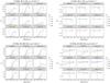 |
Fig. A.1 6.7 GHz methanol maser linear and circular polarisation fraction as a function of the maser luminosity for five different θ. The vertical line marks TBΔΩ where gΩ = 10R. Magnetic field strength is 1 and 100 mG, thermal velocity width is 1 km s−1 and the hyperfine transitions are indicated in each panel. The panel at the top left labelled “baseline” indicates a fixed pumping rate equal for all the hyperfine transitions, while all others assume a 10× preferred pumping for the indicated i → j transition. |
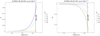 |
Fig. A.2 6.2 GHz methanol maser baseline. Linear and circular polarisation fraction as a function of the maser luminosity for five different θ. The vertical line marks TBΔΩ where gΩ = 10R. Magnetic field strength is 10 mG, thermal velocity width is 1 km s−1. |
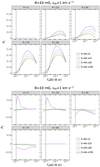 |
Fig. A.3 6.7GHz methanol maser linear and circular polarisation fraction as a function of the maser luminosity. Colours indicate different degrees of preferred pumping (3, 10, 30, 100 times) for the hyperfine transition 3 → 4 A. The vertical dotted lines indicate gΩ = 10R. Magnetic field strength, angle θ, and thermalwidth are indicated in the plot. |
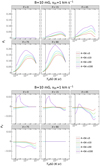 |
Fig. A.4 6.7GHz methanol maser linear and circular polarisation fraction as a function of the maser luminosity. Colours indicate different degrees of preferred pumping (3, 10, 30, 100 times) for the hyperfine transition 4 → 5 A. The vertical dotted lines indicate gΩ = 10R. Magnetic field strength, angle θ, and thermalwidth are indicated in the plot. |
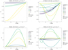 |
Fig. A.5 Circular polarisation fraction as a function of θ for different TBΔΩ, for 6.2, 6.7, 25 and 45 GHz methanol maser baselines. Magnetic field strength is 10 mG, thermal velocity width is 1 km s−1. For the 6.2 GHz methanol maser, the TBΔΩ corresponding to the gΩ = 10R limit is ~ 2 × 10¹⁰ K sr; for the 6.7 GHz methanol maser TBΔΩ corresponding to gΩ = 10R is ~ 1010 K sr; for the 25 GHz methanol maser TBΔΩ corresponding to gΩ = 10R is ~ 109 K sr; for the 45 GHz methanol maser, the TBΔΩ corresponding to gΩ = 10R is ~ 9 × 10⁸ K sr. |
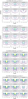 |
Fig. A.6 6.7 GHz methanol maser linear polarisation fraction PL, plotted as a function of the propagation angle θ and the rate of stimulated emission. B strengths, vth, and the preferred hyperfine transitions are indicated in each panel. The panel at the top left labelled “baseline” indicates a fixed pumping rate equal for all the hyperfine transitions, while all others assume a 10× preferred pumping for the indicated i → j transition. |
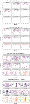 |
Fig. A.7 6.7 GHz methanol maser circular polarisation fraction PV, plotted as a function of the propagation angle θ and the rateof stimulated emission. Panels as in Fig. A.6 |
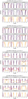 |
Fig. A.8 6.7 GHz methanol maser linear polarisation angle ψ, plotted as a function of the propagation angle θ and the rate of stimulated emission. Contours are plotted every 20°. Panels as in Fig. A.6 |
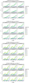 |
Fig. A.9 6.7 GHz methanol maser linear polarisation fraction, plotted as a function of the propagation angle θ for different brightness temperatures. B strength, vth, and the preferred hyperfine transitions are indicated in each panel. The panel at the top left labelled “baseline” indicates a fixed pumping rate equal for all the hyperfine transitions, while all others assume a 10× preferred pumping for the indicated i → j transition. |
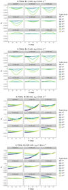 |
Fig. A.10 6.7 GHz methanol maser circular polarisation fraction PV, plotted as a function of the propagation angle θ for different brightness temperatures. Panels as in Fig. A.9. |
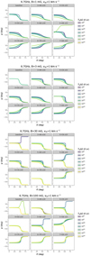 |
Fig. A.11 6.7 GHz methanol maser linear polarisation angle ψ, plotted as a function of the propagation angle θ for different brightness temperatures. Panels as in Fig. A.9. |
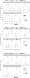 |
Fig. A.12 6.7 GHz methanol maser spectra for different levels of saturation, considering all the hyperfine transitions equally pumped. Simulations were performed for stokes I, Q, U, and V, and propagation angles θ of 0, 15, 45, 75, and 90. |
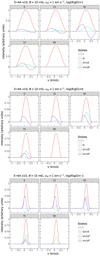 |
Fig. A.13 6.7 GHz methanol maser spectra for different levels of saturation. Simulations were performed for Stokes I, Q, U, and V, and propagation angles θ of 0, 15, 45, 75, and 90. Preferred pumping on the 3 → 4A hyperfine transition was applied. |
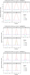 |
Fig. A.14 6.7 GHz methanol maser spectra for different levels of saturation. Simulations were performed for Stokes I, Q, U, and V, and for propagation angles θ of 0, 15, 45, 75, and 90. Preferred pumping on the 7 → 8A hyperfine transition was applied. |
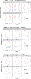 |
Fig. A.15 6.2 GHz methanol maser spectra for different intrinsic thermal velocity width. Simulations were performed for Stokes I, Q, U, and V, and for propagation angles θ of 0, 15, 45, 75, and 90. |
References
- Breen, S. L., Sobolev, A. M., Kaczmarek, J. F., et al. 2019, ApJ, 876, L25 [CrossRef] [Google Scholar]
- Burns, J. O., Owen, F. N., & Rudnick, L. 1979, AJ, 84, 1683 [NASA ADS] [CrossRef] [Google Scholar]
- Caswell, J. L., Kramer, B. H., & Reynolds, J. E. 2011, MNRAS, 414, 1914 [CrossRef] [Google Scholar]
- Crutcher, R. M., & Kemball, A. J. 2019, Front. Astron. Space Sci., 6, 66 [NASA ADS] [CrossRef] [Google Scholar]
- Dall’Olio, D., Vlemmings, W. H. T., Surcis, G., et al. 2017, A&A, 607, A111 [NASA ADS] [CrossRef] [EDP Sciences] [Google Scholar]
- Dinh-v-Trung. 2009, MNRAS, 399, 1495 [NASA ADS] [CrossRef] [Google Scholar]
- Etoka, S., Cohen, R. J., & Gray, M. D. 2005, MNRAS, 360, 1162 [NASA ADS] [CrossRef] [Google Scholar]
- Fiebig, D., & Guesten, R. 1989, A&A, 214, 333 [NASA ADS] [Google Scholar]
- Fish, V. L., Reid, M. J., Menten, K. M., & Pillai, T. 2006, A&A, 458, 485 [NASA ADS] [CrossRef] [EDP Sciences] [Google Scholar]
- Green, J. A., McClure-Griffiths, N. M., Caswell, J. L., Robishaw, T., & Harvey-Smith, L. 2012, MNRAS, 425, 2530 [NASA ADS] [CrossRef] [Google Scholar]
- Houde, M. 2014, ApJ, 795, 27 [NASA ADS] [CrossRef] [Google Scholar]
- Houde, M., Hezareh, T., Jones, S., & Rajabi, F. 2013, ApJ, 764, 24 [NASA ADS] [CrossRef] [Google Scholar]
- Hunter, T. R., Brogan, C. L., MacLeod, G. C., et al. 2018, ApJ, 854, 170 [NASA ADS] [CrossRef] [Google Scholar]
- Lankhaar, B., & Vlemmings, W. 2019, A&A, 628, A14 [NASA ADS] [CrossRef] [EDP Sciences] [Google Scholar]
- Lankhaar, B., & Vlemmings, W. 2020, A&A, 636, A14 [CrossRef] [EDP Sciences] [Google Scholar]
- Lankhaar, B., Groenenboom, G. C., & van der Avoird, A. 2016, J. Chem. Phys., 145, 244301 [NASA ADS] [CrossRef] [Google Scholar]
- Lankhaar, B., Vlemmings, W., Surcis, G., et al. 2018, Nat. Astron., 2, 145 [NASA ADS] [CrossRef] [Google Scholar]
- MacLeod, G. C., Sugiyama, K., Hunter, T. R., et al. 2019, MNRAS, 489, 3981 [CrossRef] [Google Scholar]
- Momjian, E., & Sarma, A. P. 2017, ApJ, 834, 168 [NASA ADS] [CrossRef] [Google Scholar]
- Momjian, E., & Sarma, A. P. 2019, ApJ, 872, 12 [CrossRef] [Google Scholar]
- Moscadelli, L., Menten, K. M., Walmsley, C. M., & Reid, M. J. 2003, ApJ, 583, 776 [NASA ADS] [CrossRef] [Google Scholar]
- Nedoluha, G. E., & Watson, W. D. 1990a, ApJ, 361, 653 [NASA ADS] [CrossRef] [Google Scholar]
- Nedoluha, G. E., & Watson, W. D. 1990b, ApJ, 354, 660 [NASA ADS] [CrossRef] [Google Scholar]
- Nedoluha, G. E., & Watson, W. D. 1992, ApJ, 384, 185 [NASA ADS] [CrossRef] [Google Scholar]
- Nedoluha, G. E., & Watson, W. D. 1994, ApJ, 423, 394 [NASA ADS] [CrossRef] [Google Scholar]
- Pérez-Sánchez, A. F., & Vlemmings, W. H. T. 2013, A&A, 551, A15 [NASA ADS] [CrossRef] [EDP Sciences] [Google Scholar]
- Sarma, A. P., & Momjian, E. 2009, ApJ, 705, L176 [NASA ADS] [CrossRef] [Google Scholar]
- Sarma, A. P., & Momjian, E. 2020, ApJ, 890, 6 [CrossRef] [Google Scholar]
- Sarma, A. P., Troland, T. H., & Romney, J. D. 2001, ApJ, 554, L217 [NASA ADS] [CrossRef] [Google Scholar]
- Sarma, A. P., Troland, T. H., Romney, J. D., & Huynh, T. H. 2008, ApJ, 674, 295 [NASA ADS] [CrossRef] [Google Scholar]
- Surcis, G., Vlemmings, W. H. T., Dodson, R., & van Langevelde, H. J. 2009, A&A, 506, 757 [NASA ADS] [CrossRef] [EDP Sciences] [Google Scholar]
- Surcis, G., Vlemmings, W. H. T., Curiel, S., et al. 2011a, A&A, 527, A48 [NASA ADS] [CrossRef] [EDP Sciences] [Google Scholar]
- Surcis, G., Vlemmings, W. H. T., Torres, R. M., van Langevelde, H. J., & Hutawarakorn Kramer, B. 2011b, A&A, 533, A47 [NASA ADS] [CrossRef] [EDP Sciences] [Google Scholar]
- Surcis, G., Vlemmings, W. H. T., van Langevelde, H. J., & Hutawarakorn Kramer B. 2012, A&A, 541, A47 [NASA ADS] [CrossRef] [EDP Sciences] [Google Scholar]
- Surcis, G., Vlemmings, W. H. T., van Langevelde, H. J., Hutawarakorn Kramer, B., & Quiroga-Nuñez, L. H. 2013, A&A, 556, A73 [NASA ADS] [CrossRef] [EDP Sciences] [Google Scholar]
- Surcis, G., Vlemmings, W. H. T., van Langevelde, H. J., Hutawarakorn Kramer, B., & Bartkiewicz, A. 2019, A&A, 623, A130 [CrossRef] [EDP Sciences] [Google Scholar]
- Tobin, T. L., Kemball, A. J., & Gray, M. D. 2019, ApJ, 871, 189 [NASA ADS] [CrossRef] [Google Scholar]
- Vlemmings, W. H. T. 2007, IAU Symp., 242, 37 [NASA ADS] [Google Scholar]
- Vlemmings, W. H. T. 2008, A&A, 484, 773 [NASA ADS] [CrossRef] [EDP Sciences] [Google Scholar]
- Vlemmings, W. H. T., Diamond, P. J., van Langevelde, H. J., & Torrelles, J. M. 2006, A&A, 448, 597 [NASA ADS] [CrossRef] [EDP Sciences] [Google Scholar]
- Vlemmings, W. H. T., Goedhart, S., & Gaylard, M. J. 2009, A&A, 500, L9 [NASA ADS] [CrossRef] [EDP Sciences] [Google Scholar]
- Vlemmings, W. H. T., Surcis, G., Torstensson, K. J. E., & van Langevelde H. J. 2010, MNRAS, 404, 134 [Google Scholar]
- Vlemmings, W. H. T., Torres, R. M., & Dodson, R. 2011, A&A, 529, A95 [NASA ADS] [CrossRef] [EDP Sciences] [Google Scholar]
- Watson, W. 2008, in Cosmic Agitator: Magnetic Fields in the Galaxy, 21 [Google Scholar]
- Watson, W. D., & Wyld, H. W. 2001, ApJ, 558, L55 [NASA ADS] [CrossRef] [Google Scholar]
- Western, L. R., & Watson, W. D. 1984, ApJ, 285, 158 [NASA ADS] [CrossRef] [Google Scholar]
- Wiebe, D. S., & Watson, W. D. 1998, ApJ, 503, L71 [NASA ADS] [CrossRef] [Google Scholar]
- Zeeman, P. 1897, ApJ, 5, 332 [Google Scholar]
All Tables
Methanol maser transitions considered in our simulations and observational parameters.
All Figures
|
Fig. 1 6.7 GHz methanol maser linear and circular polarisation fraction as a function of the maser luminosity for five different θ. The vertical line marks TBΔΩ where gΩ = 10R. The magnetic field strength is 10 mG, the thermal velocity width is 1 km s−1, and the preferred hyperfine transitions are indicated in each panel. The panel at the top left labelled “baseline” indicates a fixed pumping rate equal for all the hyperfine transitions, while all others assume a 10 × preferred pumping for the indicated i → j transition. The results of the simulation performed with other magnetic field strengths are given in Appendix A. |
| In the text | |
|
Fig. 2 6.7 GHz methanol maser linear polarisation fraction PL (top), circular polarisation fraction PV (middle), and linear polarisation angle ψ (bottom) plotted as a function of the propagation angle θ and the rate of stimulated emission. Stars indicate the position of the peak of PL. Magnetic field strength is 10 mG, thermal velocity width is 1 km s−1 and the hyperfine transitions are indicated in each panel. The panel at the top-left labelled “baseline” indicates a fixed pumping rate equal for all the hyperfine transitions, while all others assume a 10 × preferred pumping for the indicated i → j transition. The results of the simulation performed with other magnetic field strengths are given in Appendix A. |
| In the text | |
|
Fig. 3 6.7 GHz methanol maser linear polarisation fraction PL (top), circular polarisation fraction PV (middle) and polarisation angle ψ (bottom) plotted as a function of the propagation angle θ for different brightness temperatures. Panels as in Fig. 2. |
| In the text | |
|
Fig. A.1 6.7 GHz methanol maser linear and circular polarisation fraction as a function of the maser luminosity for five different θ. The vertical line marks TBΔΩ where gΩ = 10R. Magnetic field strength is 1 and 100 mG, thermal velocity width is 1 km s−1 and the hyperfine transitions are indicated in each panel. The panel at the top left labelled “baseline” indicates a fixed pumping rate equal for all the hyperfine transitions, while all others assume a 10× preferred pumping for the indicated i → j transition. |
| In the text | |
|
Fig. A.2 6.2 GHz methanol maser baseline. Linear and circular polarisation fraction as a function of the maser luminosity for five different θ. The vertical line marks TBΔΩ where gΩ = 10R. Magnetic field strength is 10 mG, thermal velocity width is 1 km s−1. |
| In the text | |
|
Fig. A.3 6.7GHz methanol maser linear and circular polarisation fraction as a function of the maser luminosity. Colours indicate different degrees of preferred pumping (3, 10, 30, 100 times) for the hyperfine transition 3 → 4 A. The vertical dotted lines indicate gΩ = 10R. Magnetic field strength, angle θ, and thermalwidth are indicated in the plot. |
| In the text | |
|
Fig. A.4 6.7GHz methanol maser linear and circular polarisation fraction as a function of the maser luminosity. Colours indicate different degrees of preferred pumping (3, 10, 30, 100 times) for the hyperfine transition 4 → 5 A. The vertical dotted lines indicate gΩ = 10R. Magnetic field strength, angle θ, and thermalwidth are indicated in the plot. |
| In the text | |
|
Fig. A.5 Circular polarisation fraction as a function of θ for different TBΔΩ, for 6.2, 6.7, 25 and 45 GHz methanol maser baselines. Magnetic field strength is 10 mG, thermal velocity width is 1 km s−1. For the 6.2 GHz methanol maser, the TBΔΩ corresponding to the gΩ = 10R limit is ~ 2 × 10¹⁰ K sr; for the 6.7 GHz methanol maser TBΔΩ corresponding to gΩ = 10R is ~ 1010 K sr; for the 25 GHz methanol maser TBΔΩ corresponding to gΩ = 10R is ~ 109 K sr; for the 45 GHz methanol maser, the TBΔΩ corresponding to gΩ = 10R is ~ 9 × 10⁸ K sr. |
| In the text | |
|
Fig. A.6 6.7 GHz methanol maser linear polarisation fraction PL, plotted as a function of the propagation angle θ and the rate of stimulated emission. B strengths, vth, and the preferred hyperfine transitions are indicated in each panel. The panel at the top left labelled “baseline” indicates a fixed pumping rate equal for all the hyperfine transitions, while all others assume a 10× preferred pumping for the indicated i → j transition. |
| In the text | |
|
Fig. A.7 6.7 GHz methanol maser circular polarisation fraction PV, plotted as a function of the propagation angle θ and the rateof stimulated emission. Panels as in Fig. A.6 |
| In the text | |
|
Fig. A.8 6.7 GHz methanol maser linear polarisation angle ψ, plotted as a function of the propagation angle θ and the rate of stimulated emission. Contours are plotted every 20°. Panels as in Fig. A.6 |
| In the text | |
|
Fig. A.9 6.7 GHz methanol maser linear polarisation fraction, plotted as a function of the propagation angle θ for different brightness temperatures. B strength, vth, and the preferred hyperfine transitions are indicated in each panel. The panel at the top left labelled “baseline” indicates a fixed pumping rate equal for all the hyperfine transitions, while all others assume a 10× preferred pumping for the indicated i → j transition. |
| In the text | |
|
Fig. A.10 6.7 GHz methanol maser circular polarisation fraction PV, plotted as a function of the propagation angle θ for different brightness temperatures. Panels as in Fig. A.9. |
| In the text | |
|
Fig. A.11 6.7 GHz methanol maser linear polarisation angle ψ, plotted as a function of the propagation angle θ for different brightness temperatures. Panels as in Fig. A.9. |
| In the text | |
|
Fig. A.12 6.7 GHz methanol maser spectra for different levels of saturation, considering all the hyperfine transitions equally pumped. Simulations were performed for stokes I, Q, U, and V, and propagation angles θ of 0, 15, 45, 75, and 90. |
| In the text | |
|
Fig. A.13 6.7 GHz methanol maser spectra for different levels of saturation. Simulations were performed for Stokes I, Q, U, and V, and propagation angles θ of 0, 15, 45, 75, and 90. Preferred pumping on the 3 → 4A hyperfine transition was applied. |
| In the text | |
|
Fig. A.14 6.7 GHz methanol maser spectra for different levels of saturation. Simulations were performed for Stokes I, Q, U, and V, and for propagation angles θ of 0, 15, 45, 75, and 90. Preferred pumping on the 7 → 8A hyperfine transition was applied. |
| In the text | |
|
Fig. A.15 6.2 GHz methanol maser spectra for different intrinsic thermal velocity width. Simulations were performed for Stokes I, Q, U, and V, and for propagation angles θ of 0, 15, 45, 75, and 90. |
| In the text | |
Current usage metrics show cumulative count of Article Views (full-text article views including HTML views, PDF and ePub downloads, according to the available data) and Abstracts Views on Vision4Press platform.
Data correspond to usage on the plateform after 2015. The current usage metrics is available 48-96 hours after online publication and is updated daily on week days.
Initial download of the metrics may take a while.