| Issue |
A&A
Volume 644, December 2020
|
|
|---|---|---|
| Article Number | A69 | |
| Number of page(s) | 15 | |
| Section | Catalogs and data | |
| DOI | https://doi.org/10.1051/0004-6361/201834122 | |
| Published online | 01 December 2020 | |
The Northern Extragalactic WISE × Pan-STARRS (NEWS) catalogue
Machine-learning identification of 40 million extragalactic objects⋆
Institute of Astronomy, V. N. Karazin Kharkiv National University, 35 Sumska Str., Kharkiv, Ukraine
e-mail: This email address is being protected from spambots. You need JavaScript enabled to view it.
, This email address is being protected from spambots. You need JavaScript enabled to view it.
, This email address is being protected from spambots. You need JavaScript enabled to view it.
Received:
22
August
2018
Accepted:
21
August
2020
Abstract
This study involves two photometric catalogues, AllWISE and Pan-STARRS Data Release 1, which were cross-matched to identify extragalactic objects among the common sources of these catalogues. To separate galaxies and quasars from stars, we created a machine-learning model that is trained on photometric (in fact, colour-based) information from the optical and infrared wavelength ranges. The model is based on three important procedures: the construction of the autoencoder artificial neural network, separation of galaxies and quasars from stars with a support vector machine (SVM) classifier, and cleaning of the AllWISE × PS1 sample to remove sources with abnormal colour indices using a one-class SVM. As a training sample, we employed a set of spectroscopically confirmed sources from the Sloan Digital Sky Survey Data Release 14. Having applied the classification model to the data of crossing the AllWISE and Pan-STARRS DR1 samples, we created the Northern Extragalactic WISE × Pan-STARRS (NEWS) catalogue, containing 40 million extragalactic objects and covering 3/4 of celestial sphere up to g = 23m. Several independent classification quality tests, namely, the astrometric test along with others based on the use of data from spectroscopic surveys show similar results and indicate a high purity (∼98.0%) and completeness (> 98%) for the NEWS catalogue within the magnitude range of 19.0m < g < 22.5m. The classification quality still retains quite acceptable levels of 70% for purity and 97% for completeness for the brightest and faintest objects from this magnitude range. In addition, validation with external data sets has demonstrated the need for using only those sources in the NEWS catalogue that are outside the zone with the enhanced extinction. We show that the number of quasars from the NEWS catalogue identified in Gaia DR2 exceeds the number of quasars previously identified in Gaia DR2 with the use of the AllWISEAGN catalogue. These quasars may be used in future as an additional sample for testing and anchoring the Gaia Celestial Reference Frame.
Key words: methods: data analysis / catalogs / galaxies: statistics / reference systems
The catalogue is only available at the CDS via anonymous ftp to cdsarc.u-strasbg.fr (130.79.128.5) or via http://cdsarc.u-strasbg.fr/viz-bin/cat/J/A+A/644/A69
© ESO 2020
1. Introduction
In modern astrometry, a quasi-inertial celestial reference frame is set using the radio positions of extragalactic objects, which is referred to as the International Celestial Reference Frame (ICRF, Ma & Feissel 1997; Fey et al. 2015). However, in practice, due to the insufficient number of reference sources and their low luminosity, the direct use of ICRF in positional observations in the visible spectral range has proven troublesome. With the advent of the Gaia mission (Gaia Collaboration 2016), the opportunity arose to create a celestial reference frame that would be set by the optical positions of a large number of extragalactic sources. In this case, as with the creation of ICRF, a coordinate system is set by the positions of specially selected extragalactic sources, which are postulated to be free of the rotational component in their motion (Lindegren et al. 2018).
Whereas in the ESA HIPPARCOS mission (Perryman et al. 1997), the astrometric data were limited by observations of only stars, the Gaia observations, according to the estimates by (Mignard 2012), may contain data for approximately half a million quasars and active galactic nuclei (AGN) as well as several million galaxies. The identification of extragalactic objects in the Gaia catalogue will make it possible to fix and compress the coordinate system using the high-precision positions for millions of extragalactic sources that are thousands of times greater than the number of the ICRF objects. The return of the reference system from the radio to optical wavelengths will also help avoid the difficulties involved in linking the system in the optical range to the radio positions of the ICRF objects, as described in detail in (Secrest et al. 2015).
The first step in realising such an opportunity was undertaken with the positions of ∼500 000 extragalactic point-like sources from Gaia Data Release 2 (Gaia DR2, Gaia Collaboration 2018a), obtained from a cross-matching with the ICRF-prototype (Jacobs et al. 2018) and AllWISEAGN catalogues (Secrest et al. 2015), resulting in the creation of the Gaia Celestial Reference Frame (Gaia-CRF2, Gaia Collaboration 2018b). It is evident that the number of reference objects contained in Gaia DR2 can be expanded to ∼106, which will allow, in many cases, for studies to use the reference system directly, without addressing a kinematic reference system defined by positions and proper (or spatial) motions of approximately 1.3 billion stars. In addition, there is the problem of matching the Gaia-CRF2 reference frame with the Gaia DR2 (Fedorov et al. 2011; Lindegren et al. 2018) stellar reference frame, especially in the bright part of the magnitude range (Fedorov et al. 2011; Lindegren 2020). The desire to compress the extragalactic reference system is justified, rather, since the kinematic stellar reference system, in contrast to the extragalactic system, will degrade in time due to the finite accuracy of proper motions. That is why in an era that sees the formation of the new Gaia-CRF, the creation of catalogues containing a significant number (≳106) of extragalactic sources appears not only useful, but also necessary for further improving the Gaia-CRF reference frame.
We also note that in addition to the astrometric tasks listed above, it is important that extragalactic objects be excluded from consideration in various kinematic studies of the Galaxy since they can introduce systematic biases into the final results (Pieres et al. 2020). Among these tasks, which can be solved with the use of catalogues of extragalactic sources, the following tasks are equally important: the morphological classification of galaxies (Baldry et al. 2004) and the detection of the effects of strong gravitational lensing of quasars (Spiniello et al. 2018; Khramtsov et al. 2019). With the addition of the photometric redshifts (Salvato et al. 2019), an opportunity arises for the investigation of the three-dimensional distribution of extragalactic objects (Blake & Bridle 2005), as well as a chance to compose the samples of extragalactic sources that are needed to help in the identification of host candidates for gravitational wave events (Dálya et al. 2018).
Alas, only a short list of pure extragalactic samples exists at present and it is based mainly on spectroscopic observations and covers a significant part of the celestial sphere in the optical range, that is, a sample of galaxies from the Point Source Catalogue redshift survey (PSCz, Saunders et al. 2000), Two Micron All Sky Survey (2MASS, Skrutskie et al. 2006), Redshift Survey catalogue (2MRS, Huchra et al. 2012), as well as data from the Large Sky Area Multi-Object Fibre Spectroscopic Telescope (LAMOST, Cui et al. 2012) and the Sloan Digital Sky Survey spectroscopic catalogues (SDSS, Aguado et al. 2019). Therefore, most sources observed in photometric surveys have not beeen spectroscopically confirmed to date due to the limited capabilities of modern spectrographs. The task of carrying out an efficient classification of a huge amount of sources belonging to different classes seems appears to be very important and this requires new data from various sky surveys and new methods of automatic classification.
A simple and intuitive method of classifying the sources into stars and extragalactic objects consists of using their morphological characteristics. This method, however, has significant drawbacks (Vasconcellos et al. 2011). Although the nearest galaxies are resolvable, the distant or faint galaxies, as well as quasars, look mostly like point-like objects. In addition, the effect of blending stellar images takes place in sky regions with a high source-density (for example, in the Galactic Plane). This leads to a false classification of the nearest neighbours, which are classified according to morphological features as extended sources, that is, as galaxies. Examples of the all-sky catalogues of extragalactic objects constructed with morphological criteria are: the Extended Source Catalogue (2MASS XSC, Skrutskie et al. 2006; Jarrett et al. 2000), which consists of 1.6 million extended sources, most of which are galaxies localised at z < 0.3, with a median value of the redshift, zmedian ≈ 0.1 (2MASS Photometric Redshift catalogue, Bilicki et al. 2014); a catalogue of 20 million galaxies (Peacock et al. 2016) from the SuperCOSMOS photographic survey (Hambly et al. 2001), which, in combination with the source catalogue of the space survey Wide-Field Infrared Survey Explorer (WISE, Wright et al. 2010), maps the near Universe up to z = 0.6, with zmedian ≈ 0.2 (WISE × SuperCOSMOS Photometric Redshift catalogue, Bilicki et al. 2016). Different strategies of morphological classification have been developed using data (or simulations) from the Dark Energy Survey (DES, Abbott et al. 2018), Panoramic Survey Telescope and Rapid Response System (Farrow et al. 2014), SDSS (Vasconcellos et al. 2011), Euclid (Kümmel et al. 2015), Canada-France-Hawaii Telescope Lensing Survey (CFHTLenS, Kim et al. 2015).
Another classification method is a one that uses colour indices (hereinafter, referred to as “colours”). The positions of extragalactic sources in the colour-colour or colour-magnitude diagrams differ from those of stars since the objects of different physical nature have different spectral energy distributions. For a reliable classification of objects, it is clearly not sufficient to be limited to optical magnitudes (Khramtsov et al. 2019). Therefore, the information from the optical range is often supplemented by the infrared survey data, as combining the two ranges represents spectral energy distributions much better (Krakowski et al. 2016; Nakoneczny et al. 2019; Khramtsov et al. 2019). In addition, the use of the WISE mid-infrared photometric spectral bands provides an opportunity to distinguish quasars from stars and some types of galaxies quite clearly since quasars have distinctive spectral energy distributions in the mid-infrared (see Elvis et al. 1994; Stern et al. 2005; Assef et al. 2013).
As has already been shown in numerous works, there is the possibility of separating quasars from stars with the use of only the mid-infrared photometric information (e.g. the two-colour criteria of Lacy et al. 2004; Stern et al. 2005; Donley et al. 2012 with Spitzer1 data; the two-colour criteria in Jarrett et al. 2011; Mateos et al. 2012; or the one-colour criteria proposed in Stern et al. 2012; Assef et al. 2013). However, the separation of galaxies in these colour diagrams is quite difficult as stars overlap with galaxies in the mid-infrared colour diagrams (e.g. Fig. 12 in Wright et al. 2010). Also, Kovács & Szapudi (2015) proposed an approach that allows for the identification of extragalactic objects that accounts for the colours in the near- and mid-infrared spectral ranges. With the use of the 2MASS and WISE photometry, the distinction of extragalactic objects from stars has become more reliable.
The support vector machine (SVM, Vapnik 1995) is one of the most popular geometric classifier used for the separation of objects in colour diagrams. The classification of objects into groups with the SVM is reduced to the construction of a separating hyperplane in a multidimensional parameter space describing these objects. This method has found its application in the many works dedicated to the identification of extragalactic objects, including Solarz et al. (2012), where the classification of objects on the infrared colour diagrams within the AKARI (Matsuhara et al. 2005) North Ecliptic Pole Deep Field (AKARI NEP) has been implemented. In the work by Małek et al. (2013), the SVM was used to classify objects into stars, galaxies, and quasars with their colours within optical-infrared wavelength range for the VIMOS Public Extragalactic Redshift Survey (VIPERS2). The SVM algorithm has been used in Kovács & Szapudi (2015) to analyse the colours, which contribute to the separation of objects into extragalactic sources and stars with using the 2MASS × WISE catalogue. The re-adaptation procedure for the WISE × SuperCOSMOS galaxy catalogue (Bilicki et al. 2016), performed to identify the galaxies using the SVM separation in colour space, is proposed in Krakowski et al. (2016).
We present a catalogue of candidate extragalactic objects of the Northern Extragalactic WISE × Pan-STARRS (NEWS), which covers almost 3/4 of the sky in a broad optical-IR spectral range, with a depth of up to 23m in filter g. To create the NEWS catalogue, we paired up the mid-IR data of the WISE survey (Wright et al. 2010) with those of the Pan-STARRS digital survey (Chambers et al. 2016) in the optical and near-IR spectral ranges. Our catalogue is the result of a classification of the WISE × Pan-STARRS objects with the SVM machine-learning algorithm. The classification was based solely on photometric information and the automatic creation of features was carried out using an autoencoder.
2. Data and sample selection
2.1. AllWISE
The Wide-field Infrared Survey Explorer (WISE, Wright et al. 2010) is a space NASA Medium Class Explorer mission that surveyed the whole celestial sphere in the mid-infrared wavelength range using four filters – W1, W2, W3, W4 (3.4, 4.6, 12, and 22 μm, respectively, with angular resolutions of 6.1″, 6.4″, 6.5″, and 12″ in these bands). We used the data from the AllWISE catalogue (Cutri et al. 2013), which incorporates data from the WISE Full Cryogenic, 3-Band Cryo, and NEOWISE Post-Cryo survey phases. The AllWISE catalogue contains information (positions, magnitudes, apparent motions, variability, etc.), collected over 6−12 months, for 747.6 million sources. The catalogue is 95% complete up to W1 < 17.1m, W2 < 15.7m, W3 < 11.5m, and W4 < 7.7m (in the Vega system).
The AllWISE photometry is problematic in densely populated sky regions due to the effects of saturation and blending; detections in W1 and W2 for bright sources consist mostly of unreliable measurements. Also, the aperture photometry is problematic for the extended sources (which are not presented in the 2MASS XSC catalogue) in AllWISE because of the lack of aperture corrections on source compactness. Keeping this in mind, we selected sources with existent measurements in W1, W2 profile-fit magnitudes (that are signed in the catalogue as w1mpro and w2mpro, hereafter, W1 and W2) and limited this sample by the following criteria: snrW1 > 5, snrW2 > 2 and W1 > 13.8m, where snrW1, snrW2 represent the S/N of measurements in the W1, W2 bands, respectively. We used no information in the W3, W4 bands because of the low sensitivity. In consequence, we obtained a sample comprising 508 854 970 million objects.
2.2. Pan-STARRS DR1
The Pan-STARRS Data Release 1 catalogue (PS1, Chambers et al. 2016) is the first release of Panoramic Survey Telescope and Rapid Response System (Pan-STARRS1) located at the Haleakala Observatory. Pan-STARRS1 consists of a few surveys: roughly 81% of the observation time was dedicated to the 3π Steradian Survey (56%) and Medium Deep Survey (25%). Within the Pan-STARRS1 survey, observations of almost 30 000 sq. deg. (90° > δ > −30°), involving optical and near-infrared filters (g, r, i, z, y filters with effective wavelengths of 481, 617, 752, 866, and 962 nm, respectively), were conducted up to 23.3m, 23.2m, 23.1m, 22.3m, 21.4m in each band respectively (on the 5σ limiting sensitivity level). The PS1 catalogue consists of ≈1.9 billion sources, most of them with photometry.
We used the mean PSF magnitudes (in the AB system) from the PS1 catalogue. This choice was made on the basis of the fact that the number of the sources in PS1 with measured PSF magnitudes is larger than a number of sources with measured Kron-like magnitudes. We selected the sources within the magnitude ranges of 14m < g < 23m and 14m < r < 23m and limited the sample by the magnitude errors (σx < 0.5 mag, where x denotes one of the five filters). The reasons for selecting such limits are evident. Firstly, extragalactic sources are almost absent in the bright part of optical magnitudes (<14m). In addition, images of bright sources are saturated, leading to unrealistic estimates of magnitudes. On the other hand, a limitation by g < 23m and r < 23m results in the exclusion of the sources with low S/N. After filtering, we obtained a sample consisting of 835 713 490 objects.
2.3. Positional cross-matching
We cross-matched the two catalogues in the following way. For each of the AllWISE sources located in the centre of a circular window with a search radius of 1.5″, we selected a source from PS1 using the software described in Akhmetov et al. (2019). If two or more sources hit the window, we selected the one that was closer to the centre of the search window. In this way, we excluded all the sources from PS1 which had more than one analogue in AllWISE. To avoid falling into the sample of fast objects, close to the Sun (e.g. brown dwarfs), with the absolute value of proper motion exceeding ∼10 mas yr−1, the search window radius was chosen as equal to 1.5″ as the optimal one (PS1 and WISE observations were performed at different epochs). As a result, the photometric AllWISE × PS1 sample was obtained consisting of ∼200 million sources, each of which also have their positions from PS1, as well as seven magnitudes in optical and IR filters from PS1 and AllWISE. The resulting sample is referred to as the inference sample in this paper.
2.4. Training sample: SDSS DR14
To classify all the sources from the inference sample, we created a training sample, which is a set of objects with the known classes. Considering that any classification result directly depends on the training sample, it is clear that in training the classification algorithm, we must use a set that would be the most pure and complete (the latter pertaining to the range of types of objects). To attain such a sample, we used spectroscopically confirmed objects from the SDSS Data Release 14 catalogue (Abolfathi et al. 2018). The SDSS DR14 is the second release of phase IV of the SDSS (Blanton et al. 2017) and it is cumulative, including new data from the extended Baryon Oscillation Spectroscopic Survey (eBOSS, Dawson et al. 2016) and the results of the second phase of the Apache Point Observatory Galactic Evolution Experiment (APOGEE, Majewski et al. 2016) observations.
The SDSS DR14 catalogue contains 4 851 200 spectroscopically confirmed objects, among which 2 541 242 objects are galaxies, 680 843 are quasars, and 928 859 are stars. To improve the quality of our training sample, the list of objects was adjusted by including only those objects that were flagged in SDSS DR14 as well-confirmed (zWarning=0), and by excluding the stars corresponding to extended sources and flagged as CLASS=GALAXY. Then the objects from the corrected list were cross-matched with the inference sample in the search window of 1″ in radius. As a result, we have the SDSS × AllWISE × PS1 sample containing 1 784 610 objects with known classes and seven known magnitudes (g, r, i, z, y, W1, W2). Later in the paper, we refer to this sample as the training sample. Most of objects in the training sample are extragalactic (1 474 458 galaxies and quasars) and the rest of them (310 152) are stars. The magnitude distribution of the training sample, in comparison with the inference sample, is presented in Fig. 1. The plot shows the overlapping of magnitude distributions for the training and inference samples. This overlapping is a crucial condition with which to provide a stable classification model due to the different magnitude error distribution against the magnitude.
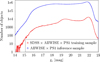 |
Fig. 1. Histogram of g magnitude distribution for the AllWISE × PS1 inference (violet) and training (orange) samples of sources. |
3. Classification model
Classification of the AllWISE × PS1 objects into galactic and extragalactic sources includes several key stages. At the first stage, we create a classification model using the training data from SDSS DR14. At the next stage, we apply the obtained model to the AllWISE × PS1 inference dataset. To correctly apply the classification model to the inference data of a larger volume than that of the training one, it is very important that some constraints be imposed on these data.
Firstly, we introduce a set of parameters for classification. These parameters must satisfy a requirement to be capable of separating the sources into two classes. We called these parameters features, as is customary in machine learning. The features may not be directly observable characteristics but should ensure the separation of objects of different classes in the best way.
The next restriction implies that the inference objects must have physical properties similar to those of the objects from the training sample. This condition is necessary to avoid classification of sources of unknown nature in AllWISE×PS1. Such sources must be excluded from consideration in the classification process. We call them off-model objects.
It is evident that for successful classification, a model must be developed that would include the above-noted restrictions. In this section, we briefly present a formal description of the classification model that allows us to classify any object if it is provided with photometric information (W1, W2 and g, r, i, z, y from AllWISE and Pan-STARRS DR1, respectively). Herein, the classification is performed using only colour indices, namely, 21 colour indices obtained from optical and infrared magnitudes.
3.1. Model description
When considering the binary classification problem, we define the classification model as a structure that is formed of an n-dimensional linear space of features  , where the separation takes place, and a hyperplane ⟨w, h⟩−b = 0 that separates objects into two groups in the feature space. Any object with the colour vector y = {y1, y2, …, ym} (where m – is a number of colours) can be unambiguously classified as d(x) = sign(⟨w, x⟩−b), where x – is a feature vector associated with the vector of colour indices by some functional transformation f, i.e. f : X → Y, Y ∈ ℝm, X ∈ ℝn. Classification can be performed only when the feature vector is in the range of features of the model: x ∈ E(h). The range of features that can be used for classification should be in the area bounded by a certain hypersurface involving the space of all objects from the training sample. Such a hypersurface can be represented by a function that is positive in the range of model features and negative elsewhere. Finally, we define the training sample as a finite set of objects with known features and classes.
Learning is the core of our classification model. By training, we mean iterative construction of a certain relationship between colours y and classes d of objects in a training sample. Training includes all the basic procedures for building a model: (1) creation of representative features for classification; (2) search for a hypersurface spanning a space that contains all representative features of the training sample; (3) construction of a hyperplane separating objects of two classes inside a space bounded by the hypersurface.
Since a vector of colours is a single initial characteristic of objects, we have to find in the training process: (1) a form of transformation from the initial space of colours to the space of features; (2) an equation of a hypersurface covering that is part of the feature space, which contains only the features of the training sample objects, and therefore excludes the use of other objects that do not have these features; (3) an equation of a separating hyperplane in the feature sub-space noted in item 2.
The location of a source with respect to the separating hyperplane in the feature space determines the its class. Sources that are outside bounding hypersurface in the feature space are assumed to be off-model.
3.2. Model construction
The model performs a probabilistic classification of objects into two classes: galactic and extragalactic. As mentioned in the previous sub-section and described in detail in Khramtsov & Akhmetov (2018), thanks to our training tool, we find: the form of the transformation of the colour space into the space of features, as well as the bounding hypersurface equation and the equation of the separating hypreplane.
In the first phase, the feature space was created, in which the location of extragalactic sources differs from the location of stars. Typically, when constructing a feature space, only some of the original colours are used for classification (Kovács & Szapudi 2015; Krakowski et al. 2016; Vickers et al. 2016; Akhmetov et al. 2017). The selection of features can be performed using various methods (e.g. with the principal component analysis). A distinctive peculiarity of our model is that instead of the manual selection of certain colours, we used the automatic creation of features that are somehow associated with all colour indices. To find informative features from a complete data set, a neural network autoencoder was used (Rumelhart et al. 1986).
An autoencoder, as the specific architecture of a neural network, consists of two parts: encoder and decoder. An autoencoder introduces data in a feature vector that has a dimension less than the input colour vector (encoding), and restores the input colour data from features (decoding). The quality of representation is determined by the accuracy of restoration of the input colours at the decoder output. The main goal of training an autoencoder within our model is to produce the most informative and uncorrelated features that are capable of most accurate representation of the initial data.
In our task, we used only the result of the encoder, while the decoder was used only for its training and for quality control of the representation. To create the feature space, we used a deep autoencoder: encoding was carried out through a four-layer network (where 21-15-10-5 are the numbers of neurons in each layer, respectively, with a non-linear connection between the layers). The encoder input was represented by 21 colours and five features were extracted from the encoder output layer.
Decoding was performed by a neural network symmetric to the encoder – 5-10-15-21. To ensure the representation of 21 colours calculated from the g, r, i, z, y, W1, W2 magnitudes, we used the data about all 1.8 million objects from the training sample. As a result of our encoding, we successfully represented a 21-dimensional colour vector by a five-dimensional feature vector for each object of the training sample, with the error of restoring the initial colours3 of the order of 10−5 mag.
In summary, we can confirm that the construction of a feature space is a process of determining five parameters that are the non-linear weighted combinations of 21 initial colours. The obtained parameters contain information about the location of stars and extragalactic objects in the initial colour diagram. To carry out the correct classification, we also performed a preliminary filtering of off-model objects in the AllWISE × PS1 using a one-class support vector machine (OCSVM, Schölkopf et al. 1999) in the feature space.
The next step in the construction of the classification model is the separation of extragalactic sources from galactic objects. To do this, we used the SVM which has found a broad application in the solving of various problems in astrophysics related to the classification of objects. The SVM classification implies a simple geometric interpretation. The algorithm accepts features and classes for training objects as an input, and at the output it provides a hyperplane equation that optimally separates the objects. By the term “optimally separating hyperplane”, we mean a hyperplane that is located between different classes and that is most distant from the nearest points of both classes.
It should be noted here that the separating hyperplane is not always optimally located with respect to the classes. Optimal separation occurs when the numbers of objects of different classes are approximately the same. Otherwise, when the training sample is unbalanced (i.e. one group is larger than another), the hyperplane shifts toward the class with fewer objects. Such a shift of the hyperplane leads to erroneously classified objects in a class that contains fewer objects, and thereby increases the pollution of a larger sample (see, for example, Kovács & Szapudi 2015). To avoid this, we used a special balancing scheme that takes into account different numbers of sources in different classes. In the case of an unequal number of objects of two classes, weighting is applied. The objects of a less numerous class are assigned a weight equal to the ratio of the number of objects of the class that is not weighted to the number of objects of the selected class. The great advantage of this approach is that it does not require any training to remove objects from the class with the largest number of objects. Indeed, we could consider more sophisticated weighting procedures, introducing the reproduction of the sources of a less numerous class by changing their locations in the feature space. Therefore, SVM training was performed using the entire training sample, which allowed us to build a hyperplane that optimally separates extragalactic objects from stars in the feature space.
4. Final catalogue of extragalactic objects
In this section, we describe the results of the identification of extragalactic objects in the whole AllWISE × PS1 sample using the classification model we created. To create the final catalogue of galaxies, we mapped the colours of each of the objects into a five-dimensional feature space, searched for off-model objects with OCSVM, and classified the objects with the SVM.
4.1. Outlier detection
After training the OCSVM in detection of anomalies, we applied it to the entire AllWISE × PS1 sample. As a result, ∼300 000 objects were identified as off-model ones. These objects were located outside the feature space region occupied by the training objects.
Most of the detected anomalies are located near the plane of the Galaxy. The detection of anomalies is necessary and important for us as a step in cleaning the inference sample. An analysis of the anomalies found in the AllWISE catalogue from photometric and morphological information (also using OCSVM), is presented by Solarz et al. (2017). Although our model can also detect reddening and interpret it as galactic absorption or reddening of extragalactic objects, an interest in the nature of the detected anomalies and their analysis are beyond the scope of this article.
4.2. Classification result
After deleting off-model objects, the remaining AllWISE × PS1 objects have been classified using the SVM. To make a decision regarding the class of a particular object of the inference sample, we used an additional parameter pxgal, implemented by the SVM classifier. In the terms of the SVM, probability pxgal is the distance of the object from the separating hyperplane expressed through the sigmoid (Platt 1999). We assumed that an object is extragalactic if the corresponding probability is pxgal > 0.5. This criterion allowed us to get a sample of candidates for extragalactic sources consisting of 40 350 492 objects. The g magnitude distribution of these sources in the NEWS catalogue reaches its maximum at g ∼ 21.7m, which shows that the catalogue of extragalactic objects we created is currently one of the deepest catalogues of galaxies covering most of the sky. Sky distribution of the sources from NEWS catalogue (Fig. 2) shows that the number of extragalactic sources is decreasing towards the Zone of Avoidance.
 |
Fig. 2. Sky distribution of 40 million objects from the NEWS catalogue in Aitoff projection (galactic coordinates with l = 0°, b = 0° at the centre). |
Our catalogue consists mostly of extended sources. We calculated the number of point sources using a quantity g − gKron, where gKron – are magnitudes derived with the Kron radius (Kron 1980) taken into account; the difference between magnitudes obtained with two different methods (PSF and Kron magnitudes) is a criterion that the source should be regarded as a point source (Farrow et al. 2014).
This difference is approximately equal to zero for point-like objects and generally greater than zero for extended sources. Pointness was established according to the following criterion: −0.25 < g − gKron < 0.05 for g < 21m; all objects that did not fall within the specified interval were considered extended. It turned out that among 38 million sources with the available gKron magnitudes in PS1 catalogue, about 2 million sources have been identified as point-like sources (see Fig. 3).
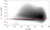 |
Fig. 3. Distribution of g − gKron versus g magnitude for 38 million objects. A cut g − gKron = 0.05 (red line) roughly separates the extended objects from the point-like objects. |
The NEWS catalogue, in addition to galaxies, contains quasars as well. Due to the peculiarities of our model construction, we are not able to separate quasars from galaxies, but this can be done post factum, using well-known criteria for identification of quasars. For example, if one of the most famous criteria for identifying quasars is used (Stern et al. 2012), namely W1 − W2 > 0.8 (W1, W2 are magnitudes in the mid-IR from WISE), then 2 286 418 quasar candidates can be identified in the NEWS catalogue, of which ∼1 000 000 meet the criterion of pointness.
We note that the sky areas with enhanced absorption can be excluded from the NEWS catalogue of galaxies due to unreliable classifications within them. This can be seen from Fig. 4: probability pxgal strongly depends on coordinates, and pxgal < 0.9 at δ < −30° and inside the avoidance zone. In the appendix, we give a test for the quality of classification as a function of absorption and show that the best quality is achieved for the colour excess values4E(B − V) < 0.2m, which are inherent to 37 445 949 sources in the NEWS catalogue.
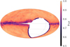 |
Fig. 4. Sky distribution of the pxgal for 40 million sources from the NEWS catalogue in Aitoff projection (galactic coordinates, l = 0°,b = 0° at the centre). |
In addition, as is shown in Krakowski et al. (2016), restriction of the WISE sample in stellar magnitude, W1 < 17m, results in the exclusion of some instrumental artefacts in the WISE catalogue. We checked the effect of this restriction on the classification quality and show in the appendix that the restriction of the sample in stellar magnitude, W1 < 17m, results in an increase in the overall quality of the NEWS catalogue data.
5. Validation with external data
Various spectroscopic surveys contain the most accurate information on the classes of the observed objects. In this regard, the catalogues containing confirmed galaxies, quasars, and stars are of particular interest to us. We refer to these classes of objects as true ones later in this paper.
For validation, it is necessary, first of all, to identify in the AllWISE × PS1 catalogue those spectroscopically confirmed galaxies and stars from various catalogues and then to compare the true classes, that is, those that have been determined from spectroscopic data, with the classes predicted by our model. This approach provides the opportunity to evaluate two main parameters – the purity and the completeness of the NEWS catalogue. To determine the purity of the NEWS catalogue, it is necessary to estimate what fraction of the total number of spectroscopically confirmed stars in AllWISE × PS1 has been identified in the NEWS catalogue. Accordingly, to determine the completeness, it is necessary to estimate what fraction of the total number of spectroscopically confirmed galaxies in AllWISE × PS1 has been identified in the NEWS catalogue.
It should be noted that, in fact, we did not calculate the purity of the NEWS catalog using the definition given above (and formalised in Sect. 5.1). This is due to the fact that the calculation of this parameter is difficult in the case of a strong imbalance in class sizes. As we show below, most of the catalogues we used contain orders of magnitude fewer stars than galaxies. This remark does not refer to completeness since, for its estimation, only quantitative information about its extragalactic sources is significant. That is why we used the Matthews correlation coefficient (MCC, Matthews 1975) to evaluate the quality of the NEWS catalogue.
Below, we briefly describe the classification quality metrics and those catalogues, along with the data we used to evaluate the classification quality performed by our model. We also discuss the results of validation. In the appendix, we provide more complete information on the testing the classification quality based on the SDSS and LAMOST samples.
5.1. Classification quality metrics
We denote the number of objects of classes A and B as NA and NB, respectively, and the number of objects of class A which were classified as the B class objects as NAB. In particular, we set the number of galaxies classified as galaxies to be designated as NGG and the number of galaxies classified as stars as NGS, and similarly for the two remaining cases. The purity PG and completeness CG of the sample of galaxies can then be determined accordingly, as:
 (1)
(1)
 (2)
(2)
With this definition, purity demonstrates what proportion of objects classified as galaxies are actually galaxies, and completeness shows what proportion of all galaxies have been classified as galaxies. The purity, PS, and completeness, CS, of a sample of stars can be introduced similarly (Soumagnac et al. 2015).
The purity metric described above is not obviously convenient for unbalanced samples. To avoid the wrong estimate of purity for a sample of galaxies, we also used a MCC, which is virtually insensitive to imbalance in class sizes:
 (3)
(3)
The MCC, as any correlation coefficient, varies in the range between −1 and 1. When all galaxies are classified as stars and all stars as galaxies, we have PG = PS = CG = CS = 0 ⟹ MCC = −1. Conversely, in the case of ideal classification, when all galaxies are classified as galaxies, and all stars are classified as stars, MCC = 1. If the classification is the result of random guessing, no correlation between the true and predicted classes will be observed, and MCC = 0. MCC characterises the quality of classification as a whole, in contrast to the purity and completeness, which show the quality of classification of each of the classes.
5.2. Spectroscopic datasets
As validation samples, we used the following catalogues of spectroscopically confirmed sources:
-
DEEP2 Data Release 4 (Newman et al. 2013);
-
Deep Imaging Multi-Object Spectrograph (DEIMOS, Hasinger et al. 2018);
-
Galaxy And Mass Assembly Data Release 3 (GAMA, Driver et al. 2011; Baldry et al. 2018);
-
LAMOST Data Release 4 (Cui et al. 2012);
-
PRIsm MUlti-object Survey Data Release 1 (PRIMUS, Coil et al. 2011);
-
SDSS DR14 (see Sect. 2.4);
-
VIPERS Data Release 2 (Scodeggio et al. 2018);
-
zCOSMOS (Davies et al. 2015).
We fulfilled the coordinate cross-matching of each of the above listed catalogues (in addition to SDSS; the reason for using the SDSS training sample as a validation sample is described in the appendix) with AllWISE × PS1 in a window with a radius of 1.0″. The results are presented in Table 1. In Fig. 5, we show a g-band magnitude distribution of the validation samples matched with the AllWISE × PS1 catalogue. This clearly shows the variation of magnitude distributions for each validation sample, allowing us to test the classification quality at the different magnitudes.
Number of stars and galaxies in the validation catalogues matched in AllWISE × PS1.
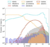 |
Fig. 5. Histogram of g magnitude distribution for the validation datasets. |
5.3. Validation with LAMOST DR4
Firstly, we analysed over 1 million sources from LAMOST DR4, which have been successfully identified with the sources from the AllWISE × PS1 test sample classified in the window with a search radius of 1.0″. Although most sources are bright enough (g < 21m) to allow us to evaluate the quality of classification only in the bright part of the magnitude range, nevertheless, weak sources up to g = 22m are also presented in the validation sample. We note in advance that the LAMOST DR4 catalogue contains the largest number of stars among the validation samples used in this work, which is very important for estimating the purity of the NEWS catalogue. Namely, cross-matching result of LAMOST DR4 and AllWISE × PS1 consists of 1 142 420 stars and 76 052 extragalactic objects. In analysing the indicated intersection, we found out that 3461 sources marked in LAMOST as stars were classified by our model as extragalactic sources.
To understand the reasons for this contradiction, we decided to find out what photometric parameters are inherent in the objects of the LAMOST sample that are marked as stars, but classified by our model as extragalactic objects. With this aim, we constructed, for these objects, a dependence between the colour W1 − W2, which is a diagnostic for separating quasars from stars and galaxies, along with the parameter g − gKron, which is useful in selecting extended objects (see Fig. 3). As seen in Fig. 6, most of these objects are either within the interval of W1 − W2 > 0.8, that is, located in the region where quasars are located or they have relatively a high value of g − gKron, which is typical of extended sources. For these objects (stars according to the LAMOST classification) located in the regions occupied by extragalactic objects, our model predicts a high probability that they belong to extragalactic objects. Therefore, we believe that these sources marked in LAMOST as stars are extragalactic with a higher probability than stars. In addition, in examining in Fig. 7 a distribution of the two first features obtained with the encoder for all the sources marked in LAMOST as stars, two distant groups of stars with a relatively high value of the second feature are clearly seen (see bottom-left panel in Fig. 7). It is obvious that they are located in the region, which is occupied by extragalactic sources (Fig. 7, to the bottom-right). At the same time, such an effect is almost not observed at all for the stars of the SDSS catalogue (see top panels in Fig. 7). The above considerations allows us to conclude that the validation sample contains false classes for some objects. It turns out that they can be fully identified, up to the classification error, with our model and based only on the colour information.
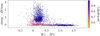 |
Fig. 6. Distribution of gPSF − gKron versus W1 − W2 colour for sources that are identified as stars in LAMOST DR4 data, but classified as extragalactic objects within our model. The probability of source being extragalactic pxgal is marked in colour. |
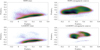 |
Fig. 7. Distribution of the first two features for the AllWISE × PS1 spectroscopically confirmed sources. Top panel: SDSS training sample; bottom panel: LAMOST validation sample. Left images correspond to the distribution of stars within first two features; right images to the distribution of extragalactic sources. |
In the next step, we performed a visual viewing of all 3461 sources in the PS1 images5 and found that they contain 1019 mixed sources (close pairs of sources), 71 sources from the regions of high image density, 832 point-like sources, and 1539 extended sources (galaxies). The majority of the mixed sources in PS1 turned out to be close image pairs composed of a galaxy and a star. At the same time, the cases when close pairs are composed of two point sources, possibly stars, are not rare as well. The classification by our model of mixed sources in AllWISE × PS1 as extragalactic is probably due to the fact that in galaxy-star pairs, the contribution to the total intensity from galaxies exceeded that of their neighbouring stars. At the same time, in observations of mixed sources in LAMOST, the coordinates of precisely those stars have been detected in most cases, resulting in mismatch of the LAMOST and NEWS classes.
After visual viewing, we removed all mixed sources (close pairs and sources from the high-density regions). We also changed classes for those LAMOST stars that are classified as extragalactic objects by our model, and assigned the class of “extragalactic” to all extended objects and class “star” to all point sources. Afterwards, the sample of differently classified objects decreased from 3461 to 832 sources. It is appropriate to note here that although visual viewing improved the quality of the sample being checked, it could not, however, ensure the reliability of the classification of point images of quasars inside LAMOST. Naturally, this has led to a slight decrease in the completeness and purity of the AllWISE × PS1 catalogue and, as a consequence, of NEWS, due to the mismatch of class predictions by our model with those in LAMOST. We can also conclude from this analysis that our classification model is somewhat weakened in classifying close pairs of sources (galaxy + star or star + star).
In addition, as is shown in Fig. 7 (bottom right), some objects of the galactic class in LAMOST are located in the region of stars (a small set in the bottom). We did not undertake a visual viewing of the images of these galaxies, but we do not rule out that they may also have been incorrectly classified in the framework of LAMOST.
We also found that in the intersection of the cleaned version of LAMOST with the SDSS DR14 training sample, a circular window with a radius of 1.0″ contains 79 507 common sources. To exclude the verification of objects that have been used to train the classifier, we removed these sources from the LAMOST validation sample and recalculated the classification quality criteria for this new sample. Since the remote objects were mostly extragalactic, classification quality criteria in the resulting sample has deteriorated due to an imbalance with regard to the sizes of various classes. In the appendix, we show more detailed validation results with LAMOST DR4 and SDSS DR14 samples, which indicate the high quality of the extragalactic objects identification in the NEWS catalogue (PG ∼ 98%÷99%, CG ∼ 98%÷99%).
5.4. Validation with galaxy catalogues
To evaluate the purity of the NEWS catalogue, we used also the catalogues of galaxies presented earlier. The ranges of magnitudes of the applied catalogues at the intersection with AllWISE × PS1 differ markedly (see Fig. 6), which provides a possibility for evaluating the classification quality in various parts of the magnitude range, from bright objects (g ∼ 17m) to faint ones (g ∼ 23m). It is worth noting that we present an estimate of the classification quality as a function of stellar magnitude. This was carried out because the accuracy of the features used for classification depends on the accuracy of magnitudes, which, in turn, decreases with increasing stellar magnitude.
To analyse the purity of the NEWS catalogue, we estimated the MCC and used the catalogues, which contained stars, in addition to extragalactic objects, namely VIPERS, DEIMOS, PRIMUS, and also SDSS and LAMOST, cleaned of the objects in common with SDSS. The catalogues DEEP2, zCOSMOS, and GAMA cannot be used to estimate the portion of stars polluting the sample of galaxies since they do not contain stars at all. To analyse the completeness of the NEWS catalogue, we used the above-listed catalogues, as well as DEEP2, zCOSMOS, and GAMA.
Figure 8 (left panel) shows the dependence of the MCC on stellar magnitude for five validation samples. The distributions of MCC in stellar magnitude seen in Fig. 8 appear to be quite consistent for objects from SDSS, LAMOST, DEIMOS, and VIPERS, exhibiting similar trends. Namely, the low quality of classification (MCC < 0.9) is observed up to g = 18m, then it becomes acceptable (MCC > 0.9) in the interval from 18.0m to 21.5m, and a monotonous decrease of the classification quality takes place between g ∼ 21.5m and 23m. The behaviour of the MCC when classifying the objects of the PRIMUS survey (an increase of the classification quality from MCC = 0.8 to MCC = 0.9 at 20m < g < 21m) differs markedly from the other four trends, possibly due to low-resolution spectroscopy of the PRIMUS survey, which leads to occasionally incorrect spectroscopic class confirmation.
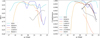 |
Fig. 8. Dependence of the MCC (left) and completeness (right) scores on g magnitude. The coloured lines represent different spectroscopic surveys, which we used to estimate the classification quality metrics. |
The sharp drops in the MCC dependencies at the edges of the magnitude range for almost every catalogue are caused by a very small number of objects in these magnitude intervals. Obviously, the smaller the total number of objects, the greater the contribution to the decrease in the MCC value from each incorrectly classified object.
We also carried out a similar procedure to study the completeness of the sample of galaxies. The result of evaluating the completeness of the NEWS catalogue as a function of stellar magnitude obtained with the use of various samples is shown in right plot of the Fig. 8. It can be seen that the completeness of the NEWS catalogue is 95% at g ∼ 18m, and larger than 99% at g ∼ 20m (from the data of the SDSS, LAMOST, GAMA, DEIMOS, and zCOSMOS surveys) and is equal to 98% at g ∼ 22.5m.
Of course, the samples used are not exhaustive since some of them contain a relatively small number of objects (∼100 ÷ 1000), with the exception of the LAMOST, SDSS (∼106), GAMA (∼105), and PRIMUS (∼104) catalogues. It is worth noting that these catalogues cover only some very limited regions of feature space (e.g. due to the selection of specific sources for spectroscopic observations), therefore, the sources they include cannot fully represent the nature variability of the objects contained in AllWISE × PS1. Thus, a validation using these catalogues cannot guarantee the exact coincidence of the purity and completeness estimates of the NEWS catalogue with their actual values. Nevertheless, despite the strong difference between the objects in these catalogues, the behaviour of the estimated classification metrics generally coincides for most samples, which is an indicator of the stability of the classification quality estimate.
5.5. Astrometric validation
Validation with external spectroscopic data provides direct consistent estimates of the purity and completeness of the NEWS catalogue. However, stars and extragalactic objects, in addition to spectroscopic features, have other features characterising their nature and the application of these features allows for a validation of a catalogue of extragalactic objects.
The proper motion of an object is one of such features. In contrast to stars, extragalactic objects are “motionless” sources in the sky because of their remoteness. At an accuracy level of about ∼1 mas, the positions of such objects can be considered as time-independent for approximately 100 years. Indeed, the galaxies are so remote that even if their tangential velocities were equal to the Hubble expansion V = H0 d the resulting proper motion (for example, for the nearest galaxy, the Andromeda nebula, located at a distance of 770 kpc, Karachentsev et al. 2004), would be less than μ0 ∼ 10−5 arcsec yr−1 at the value of assuming H0 = 70 km s−1 Mpc−1 (Freedman et al. 2001). And although the observed values of the peculiar velocities of galaxies can reach thousands of km s−1, their relative contribution against the Hubble expansion is constantly decreasing and the cosmological expansion is clearly detected starting from a distance of several Mpc (Chernin 2001). Therefore, it is obvious that any rotation of the system of galaxies caused by their peculiar velocities will be less than μ0. The data from the second release of the Gaia astrometric mission (Gaia DR2, Gaia Collaboration 2018a,b; Lindegren et al. 2018) is an excellent platform for testing the objects of the NEWS catalogue for “immobility”.
For our analysis, we used the solid-body rotation model:
 (4)
(4)
where ωx, ωy, ωz – are the components of the rotation vector and μα, μδ – are the components of proper motion.
If the NEWS catalogue really contains extragalactic sources (quasars and galaxies), then there should be no rotation of the system defined by the positions and proper motions of these sources relative to the Gaia DR2 reference frame. If the resulting rotation components are non-zero, then the sample can be assumed to contain a certain fraction of stars.
An important feature of the Gaia DR2 catalogue is the fact that it contains only point-like sources (Robin et al. 2012). Therefore, in cross-matching the NEWS catalogue with Gaia DR2, we will get a sample of point sources, which would contain only quasars and, in the case of a false classification, stars as well. This provides us with the possibility of evaluating the pollution of the NEWS catalogue by stars.
In the Gaia DR2 catalogue, proper motions and parallaxes are shown only for objects for which: (1) mean G-band stellar magnitude G < 21m, (2) astrometric_sigma5d_max < 1.2 × γ(G), where astrometric_sigma5d_max – is the largest semi-axis of the five-dimensional error ellipsoid (corresponding to the errors of five astrometric parameters), and γ(G) = max[1, 100.2(G − 18)] (Lindegren et al. 2018).
In cross-matching the NEWS catalogue with the Gaia DR2 objects satisfying these conditions, 4.3 million common objects have been found in a window with a radius of 0.5″. A majority of galaxies identified in Gaia DR2 have large errors of determining the photo-centre, and only positions are indicated for these objects. Therefore, we formed a sample containing 1 242 635 extragalactic sources for which in Gaia DR2: (a) the measured proper motions are indicated; (b) the sources are located in the sky region with δ = −30°; and (c) the sources are outside the zone with the enhanced absorption (E(B − V) < 0.1m).
Thus, 95% of the matched sources are at g < 21.6m. Accordingly, the NEWS catalogue, apart from the objects inside the Zone of Avoidance (E(B − V)> 0.1m), consists of 20.05M sources up to the g = 21.6m stellar magnitude.
Assuming our sample consists only of extragalactic objects, we expect that zero values of the rotation vector components will be obtained when using the solid-body rotation model. In Fig. 9 (left plot) we present the G-band magnitude dependencies of the rotation vector components of the coordinate system defined by the positions and proper motions of the 1.2 million sources from our sample. The values of the rotation vector components ωx, ωy, ωz reach (−0.8, −0.1, 0.6) mas yr−1 at G = 17m, (−0.4, 0.0, 0.3) mas yr−1 at G = 19m, and (−0.3, 0, 0.2) mas yr−1 at G = 21m. The behaviour of the rotation vector components demonstrates a pronounced dependence on stellar magnitude. The reason for this behaviour can be either the influence of the magnitude equation on the proper motions, or the presence of stars with noticeable proper motions in the sample. Even if the magnitude equation does exist in the Gaia DR2 data, its effect, due to the relatively uniform distribution of objects over the sky, should be of a random character rather than systematic. Therefore, we regard that the reason for the magnitude dependence is the presence of stars with noticeable proper motions in the sample we used.
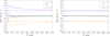 |
Fig. 9. Left: dependence of the components of the rotation vector, ωx, ωy, ωz, of the system, defined by the positions and proper motions of 1.2M NEWS sources with respect to the Gaia-CRF2 on the G magnitude. Right: dependence of components of rotation vector, ωx, ωy, ωz, of the system, defined by the positions and proper motions of 1.0M NEWS sources, passed astrometric criterion, with respect to the Gaia-CRF2 on the G magnitude. Vertical error bars represent the dispersion of components within the magnitude bin. The components ωx, ωz were shifted by ±1.0 mas yr−1 for better visibility. |
To exclude the presence of stars in the sample, we used the criterion proposed in Lindegren et al. (2018):
 (5)
(5)
which allows us to select only “motionless” sources. We selected, from the sample consisting of 1.2 million sources, those objects with the Gaia DR2 proper motions meeting this criterion as well as objects that have a probability that supports their belonging to the extragalactic class larger than 0.95; thus, our sample was reduced to 1 019 687 extragalactic objects. Repeating the procedure of determining the rotation vector components in dependence on stellar magnitude for this sample (see Eq. (4)), we found out that the magnitude dependence has become weaker and that the values of the rotation vector components are virtually zero in the entire magnitude range (see right plot in Fig. 9). We note that the actual probability limit was chosen as a compromise between the purity of the resulting sample and its completeness.
The result of this procedure can be translated into a quantitative estimate of the purity of the NEWS catalogue, assuming that many galaxies of the NEWS catalogue have not been identified in Gaia DR2 due to their extended character. This assumption is based on the fact that the Gaia observational strategy was aimed at measuring point sources only (Robin et al. 2012). Then, taking the quantity 20.05M as the total number of galaxies and stars up to g = 21.6m in the NEWS catalogue, (we determined this limit as that one, which contains 95% of the sources identified between NEWS and Gaia) and also assuming that ∼220 000 objects that did not meet the above astrometric criterion are stars, the purity of the NEWS catalogue can be calculated as PG = (20.05−0.22)/20.05 ≈ 98.9% (Eq. (1)). From this, we can conclude that the astrometric test shows an estimate of the purity of the NEWS catalogue consistent with the estimates made from external astrometric catalogues.
We note that the sample of extragalactic objects identified in Gaia DR2, consists mainly of quasars. This follows from the criterion W1 − W2 > 0.8 (Stern et al. 2012), which helps to separate quasars from objects of other types. The number of quasars among 1.2 million identified objects is ∼770 000. This quantity exceeds the number of quasars previously identified in Gaia DR2 with the use of the AllWISEAGN catalogue (Secrest et al. 2015), although the NEWS quasars cover only half the sky (due to restrictions on the declination of the PS1 survey and due to the exclusion of sky regions with the enhanced absorption), while quasars from AllWISEAGN cover the entire celestial sphere. We carried out the coordinate cross-matching of our sample of quasars with the quasars identified using AllWISEAGN, and found 505 320 quasars contained in Gaia DR2 that have not been used to create the reference frame. It is possible that these quasars may be later used as an additional sample for testing and updating the Gaia-CRF.
6. Conclusions
In this paper, we present the NEWS catalogue, which includes 40 350 492 extragalactic objects candidates (galaxies and quasars) that have passed classification based on the proposed classification model. The NEWS catalogue covers 3/4 of the celestial sphere up to g = 23m and is one of the deepest of all the available catalogues of extragalactic objects that cover a large portion of the sky.
We managed to carry out a highly precise identification of extragalactic objects in the AllWISE × PS1 sample, confirmed by a number of tests. Namely, using independent external data – catalogues of spectroscopically confirmed sources and the astrometric catalogue Gaia DR2 – we obtained high values support the purity of the NEWS sample (MCC > 0.95 at 19m < g < 21.5m with the spectroscopic data, PG ∼ 99% at 17m < g < 21.6m with the Gaia DR2, PG ∼ 98%÷99% at 17m < g < 22m with the LAMOST DR4, and PG ∼ 99% at 15m < g < 23m with the SDSS DR14 data), and high values for the completeness (CG > 99% at 18m < g < 21.5m).
The proposed method for identifying extragalactic sources is flexible and fully automatic, and it can become an alternative to traditional colour cuts with manually selected colours for classifying sources into two classes: stars and extragalactic sources. Using our classification model, we created the NEWS catalogue, which can be used for cosmological, astrophysical, and astrometric studies. In the near future, the classification model will be applied to photometric catalogues, such as the Pan-STARRS DR2 (Flewelling 2018) and unWISE catalogues (Schlafly et al. 2019).
Considering mean squared error:  , where Xi, X̃i – original and recovered colours respectively, N – number of sources.
We used extinction maps presented in Schlegel et al. (1998).
Acknowledgments
We thank the anonymous referee for the valuable and constructive comments, which have helped to improve this paper. This publication makes use of data products from the Wide-field Infrared Survey Explorer, which is a joint project of the University of California, Los Angeles, and the Jet Propulsion Laboratory/California Institute of Technology, and NEOWISE, which is a project of the Jet Propulsion Laboratory/California Institute of Technology. WISE and NEOWISE are funded by the National Aeronautics and Space Administration. The Pan-STARRS1 Surveys (PS1) and the PS1 public science archive have been made possible through contributions by the Institute for Astronomy, the University of Hawaii, the Pan-STARRS Project Office, the Max-Planck Society and its participating institutes, the Max Planck Institute for Astronomy, Heidelberg and the Max Planck Institute for Extraterrestrial Physics, Garching, The Johns Hopkins University, Durham University, the University of Edinburgh, the Queen’s University Belfast, the Harvard-Smithsonian Center for Astrophysics, the Las Cumbres Observatory Global Telescope Network Incorporated, the National Central University of Taiwan, the Space Telescope Science Institute, the National Aeronautics and Space Administration under Grant No. NNX08AR22G issued through the Planetary Science Division of the NASA Science Mission Directorate, the National Science Foundation Grant No. AST-1238877, the University of Maryland, Eotvos Lorand University (ELTE), the Los Alamos National Laboratory, and the Gordon and Betty Moore Foundation. Funding for the Sloan Digital Sky Survey IV has been provided by the Alfred P. Sloan Foundation, the US Department of Energy Office of Science, and the Participating Institutions. SDSS-IV acknowledges support and resources from the Center for High-Performance Computing at the University of Utah. The SDSS web site is www.sdss.org. SDSS-IV is managed by the Astrophysical Research Consortium for the Participating Institutions of the SDSS Collaboration including the Brazilian Participation Group, the Carnegie Institution for Science, Carnegie Mellon University, the Chilean Participation Group, the French Participation Group, Harvard-Smithsonian Center for Astrophysics, Instituto de Astrofísica de Canarias, The Johns Hopkins University, Kavli Institute for the Physics and Mathematics of the Universe (IPMU)/University of Tokyo, Lawrence Berkeley National Laboratory, Leibniz Institut für Astrophysik Potsdam (AIP), Max-Planck-Institut für Astronomie (MPIA Heidelberg), Max-Planck-Institut für Astrophysik (MPA Garching), Max-Planck-Institut für Extraterrestrische Physik (MPE), National Astronomical Observatories of China, New Mexico State University, New York University, University of Notre Dame, Observatário Nacional/MCTI, The Ohio State University, Pennsylvania State University, Shanghai Astronomical Observatory, United Kingdom Participation Group, Universidad Nacional Autónoma de México, University of Arizona, University of Colorado Boulder, University of Oxford, University of Portsmouth, University of Utah, University of Virginia, University of Washington, University of Wisconsin, Vanderbilt University, and Yale University. Guoshoujing Telescope (the Large Sky Area Multi-Object Fiber Spectroscopic Telescope LAMOST) is a National Major Scientific Project built by the Chinese Academy of Sciences. Funding for the project has been provided by the National Development and Reform Commission. LAMOST is operated and managed by the National Astronomical Observatories, Chinese Academy of Sciences. Acknowledgment – Funding for the DEEP2 Galaxy Redshift Survey has been provided by NSF grants AST-95-09298, AST-0071048, AST-0507428, and AST-0507483 as well as NASA LTSA grant NNG04GC89G. GAMA is a joint European-Australasian project based around a spectroscopic campaign using the Anglo-Australian Telescope. The GAMA input catalogue is based on data taken from the Sloan Digital Sky Survey and the UKIRT Infrared Deep Sky Survey. Complementary imaging of the GAMA regions is being obtained by a number of independent survey programmes including GALEX MIS, VST KiDS, VISTA VIKING, WISE, Herschel-ATLAS, GMRT and ASKAP providing UV to radio coverage. GAMA is funded by the STFC (UK), the ARC (Australia), the AAO, and the participating institutions. The GAMA website is http://www.gama-survey.org/. Funding for PRIMUS is provided by NSF (AST-0607701, AST-0908246, AST-0908442, AST-0908354) and NASA (Spitzer-1356708, 08-ADP08-0019, NNX09AC95G). This research has made use of the zCosmos database, operated at CeSAM/LAM, Marseille, France. We kindly request all papers using VIPERS data to add the following text to their acknowledgment section: This paper uses data from the VIMOS Public Extragalactic Redshift Survey (VIPERS). VIPERS has been performed using the ESO Very Large Telescope, under the “Large Programme” 182.A-0886. The participating institutions and funding agencies are listed at http://vipers.inaf.it. This work has made use of data from the European Space Agency (ESA) mission Gaia (https://www.cosmos.esa.int/gaia), processed by the Gaia Data Processing and Analysis Consortium (DPAC, https://www.cosmos.esa.int/web/gaia/dpac/consortium). Funding for the DPAC has been provided by national institutions, in particular the institutions participating in the Gaia Multilateral Agreement. This work has made use of the TOPCAT (Taylor 2005) data mining and visualisation software, scikit-learn (scikit-learn.org), KERAS (keras.io), sfdmap (github.com/kbarbary/sfdmap) PYTHON packages.
References
- Abbott, T., Abdalla, F., Allam, S., et al. 2018, ApJS, 239, 18 [Google Scholar]
- Abolfathi, B., Aguado, D., Aguilar, G., et al. 2018, ApJS, 235, 42 [Google Scholar]
- Aguado, D. S., Ahumada, R., Almeida, A., et al. 2019, ApJS, 240, 23 [Google Scholar]
- Akhmetov, V., Fedorov, P., Velichko, A., & Shulga, V. 2017, MNRAS, 469, 763 [NASA ADS] [Google Scholar]
- Akhmetov, V., Khlamov, S., & Dmytrenko, A. 2019, Adv. Intell. Syst. Comput., 1080, 896 [Google Scholar]
- Assef, R. J., Stern, D., Kochanek, C. S., et al. 2013, ApJ, 772, 26 [Google Scholar]
- Baldry, I. K., Glazebrook, K., Brinkmann, J., et al. 2004, ApJ, 600, 681 [Google Scholar]
- Baldry, I. K., Liske, J., Brown, M. J. I., et al. 2018, MNRAS, 474, 3875 [Google Scholar]
- Bilicki, M., Jarrett, T., Peacock, J., et al. 2014, ApJS, 210, 9 [Google Scholar]
- Bilicki, M., Peacock, J., Jarrett, T., et al. 2016, ApJ, 225, 5 [Google Scholar]
- Blanton, M., Bershady, M., Abolfathi, B., et al. 2017, AJ, 154, 28 [Google Scholar]
- Blake, C., & Bridle, S. 2005, MNRAS, 363, 1329 [Google Scholar]
- Bradley, A. 1997, Pattern Recognit., 30, 1145 [Google Scholar]
- Chambers, K., Magnier, E., Metcalfe, N., et al. 2016, ArXiv e-prints [arXiv:1612.05560] [Google Scholar]
- Chernin, A. D. 2001, Phys. Usp., 44, 1099 [Google Scholar]
- Coil, A. L., Blanton, M. R., Burles, S. M., et al. 2011, ApJ, 741, 8 [Google Scholar]
- Cui, X. Q., Zhao, Y. H., Chu, Y. Q., et al. 2012, Res. Astron. Astrophys., 12, 1197 [Google Scholar]
- Cutri, R., Wright, E., Conrow, T., et al. 2013, Explanatory Supplement to the AllWISE Data Release Products [Google Scholar]
- Dálya, G., Galgóczi, G., Dobos, L., et al. 2018, MNRAS, 479, 2374 [Google Scholar]
- Davies, L. J. M., Driver, S. P., Robotham, A. S. G., et al. 2015, MNRAS, 447, 1014 [Google Scholar]
- Dawson, K., Kneib, J.-P., Percival, W., et al. 2016, AJ, 151, 44 [Google Scholar]
- Donley, J. L., Koekemoer, A. M., Brusa, M., et al. 2012, ApJ, 748, 142 [Google Scholar]
- Driver, S. P., Hill, D. T., Kelvin, L. S., et al. 2011, MNRAS, 413, 971 [Google Scholar]
- Elvis, M., Wilkes, B. J., McDowell, J. C., et al. 1994, ApJS, 95, 1 [Google Scholar]
- Farrow, D. J., Cole, S., Metcalfe, N., et al. 2014, MNRAS, 437, 748 [Google Scholar]
- Fedorov, P. N., Akhmetov, V. S., & Bobylev, V. V. 2011, MNRAS, 416, 403 [NASA ADS] [Google Scholar]
- Fey, A. L., Gordon, D., Jacobs, C. S., et al. 2015, AJ, 150, 58 [Google Scholar]
- Flewelling, H. 2018, Astron. Astrophys. Space, 231, 436.01 [Google Scholar]
- Freedman, W. L., Madore, B. F., Gibson, B. K., et al. 2001, ApJ, 553, 47 [Google Scholar]
- Gaia Collaboration (Prusti, T., et al.) 2016, A&A, 595, A1 [NASA ADS] [CrossRef] [EDP Sciences] [Google Scholar]
- Gaia Collaboration (Brown, A., et al.) 2018a, A&A, 616, A1 [NASA ADS] [CrossRef] [EDP Sciences] [Google Scholar]
- Gaia Collaboration (Mignard, F., et al.) 2018b, A&A, 616, A14 [NASA ADS] [CrossRef] [EDP Sciences] [Google Scholar]
- Hambly, N., MacGillivray, H., Read, M., et al. 2001, MNRAS, 326, 1279 [Google Scholar]
- Hasinger, G., Capak, P., Salvato, M., et al. 2018, ApJ, 858, 77 [Google Scholar]
- Huchra, J., Macri, L., Masters, K., et al. 2012, ApJS, 199, 26 [Google Scholar]
- Jacobs, C., Charlot, P., Arias, E. F., et al. 2018, COSPAR Meeting, 42nd COSPAR Scientific Assembly, 42, B2.1-31-18 [Google Scholar]
- Jarrett, T. H., Chester, T., Cutri, R., et al. 2000, AJ, 119, 2498 [Google Scholar]
- Jarrett, T. H., Cohen, M., Masci, F., et al. 2011, ApJ, 735, 112 [Google Scholar]
- Karachentsev, I. D., Karachentseva, V. E., Huchtmeier, W. K., & Makarov, D. I. 2004, AJ, 127, 2031 [Google Scholar]
- Khramtsov, V., & Akhmetov, V. 2018, Proceedings of a IEEE XIIIth International Scientific and Technical Conference “CSIT”, 72 [Google Scholar]
- Khramtsov, V., Sergeyev, A., Spiniello, C., et al. 2019, A&A, 632, A56 [EDP Sciences] [Google Scholar]
- Kim, E., Brunner, R., & Kind, M. 2015, MNRAS, 453, 507 [Google Scholar]
- Kingma, D. P., & Ba, J. 2014, ArXiv e-prints [arXiv:1412.6980] [Google Scholar]
- Kovács, A., & Szapudi, I. 2015, MNRAS, 448, 1305 [Google Scholar]
- Krakowski, T., Małek, K., Bilicki, M., et al. 2016, A&A, 596, A39 [NASA ADS] [CrossRef] [EDP Sciences] [Google Scholar]
- Kron, R. G. 1980, ApJS, 43, 305 [Google Scholar]
- Kümmel, M., Mohr, J., Fontana, A., et al. 2015, ASP Conf. Ser., 495, 249 [Google Scholar]
- Lacy, M., Storrie-Lombardi, L. J., Sajina, A., et al. 2004, ApJS, 154, 166 [Google Scholar]
- Lindegren, L. 2020, A&A, 633, A1 [NASA ADS] [CrossRef] [EDP Sciences] [Google Scholar]
- Lindegren, L., Hernandez, J., & Bombrun, A. 2018, A&A, 616, A2 [NASA ADS] [CrossRef] [EDP Sciences] [Google Scholar]
- Ma, C., & Feissel, M. 1997, IERS Technical Note, 23 [Google Scholar]
- Majewski, S., APOGEE Team,& APOGEE-2 Team 2016, Astron. Nachr., 337, 863 [NASA ADS] [CrossRef] [Google Scholar]
- Mateos, S., Alonso-Herrero, A., Carrera, F. J., et al. 2012, MNRAS, 426, 3271 [NASA ADS] [CrossRef] [Google Scholar]
- Matsuhara, H., Shibai, H., Onaka, T., & Usui, F. 2005, Adv. Space Res., 36, 1091 [CrossRef] [Google Scholar]
- Matthews, B. 1975, Biochimica et Biophysica Acta (BBA) – Protein Structure, 405, 442 [CrossRef] [Google Scholar]
- Małek, K., Solarz, A., Pollo, A., et al. 2013, A&A, 557, A16 [NASA ADS] [CrossRef] [EDP Sciences] [Google Scholar]
- Mignard, F. 2012, Mem. Soc. Astron. It., 83, 918 [NASA ADS] [Google Scholar]
- Nakoneczny, S., Bilicki, M., Solarz, A., et al. 2019, A&A, 624, A13 [NASA ADS] [CrossRef] [EDP Sciences] [Google Scholar]
- Newman, J. A., Cooper, M. C., Davis, M., et al. 2013, ApJS, 208, 5 [Google Scholar]
- Peacock, J., Hambly, N., Bilicki, M., et al. 2016, MNRAS, 462, 2085 [NASA ADS] [CrossRef] [Google Scholar]
- Perryman, M., Lindegren, L., Kovalevsky, J., et al. 1997, A&A, 323, L49 [Google Scholar]
- Pieres, A., Girardi, L., Balbinot, E., et al. 2020, MNRAS, 497, 1547 [CrossRef] [Google Scholar]
- Platt, J. C. 1999, in Advances in Large Margin Classifiers, eds. A. J. Smola, P. Bartlett, B. Schölkopf, & D. Schuurmans (Cambridge, USA: MIT Press), 61 [Google Scholar]
- Rumelhart, D. E., Hinton, G. E., & Williams, R. J. 1986, in Parallel Distributed Processing: Explorations in the Microstructure of Cognition, eds. D. E. Rumelhart, J. L. McClelland, & CORPORATE PDP Research Group (Cambridge, USA: MIT Press), 1, 318 [Google Scholar]
- Robin, A., Luri, X., Reylé, C., et al. 2012, A&A, 543, A100 [NASA ADS] [CrossRef] [EDP Sciences] [Google Scholar]
- Salvato, M., Ilbert, O., & Hoyle, B. 2019, Nat. Astron., 3, 212 [NASA ADS] [CrossRef] [Google Scholar]
- Saunders, W., Sutherland, W. J., Maddox, S. J., et al. 2000, MNRAS, 317, 55 [NASA ADS] [CrossRef] [Google Scholar]
- Saxe, A., McClelland, J., & Ganguli, S. 2013, ArXiv e-prints [arXiv:1312.6120] [Google Scholar]
- Schlafly, E. F., Meisner, A. M., & Green, G. M. 2019, ApJS, 240, 30 [Google Scholar]
- Schlegel, D., Finkbeiner, D., & Davis, M. 1998, ApJ, 500, 525 [NASA ADS] [CrossRef] [Google Scholar]
- Schölkopf, B., Smola, A., & Müller, K. 1999, in Advances in Kernel Methods, eds. B. Schölkopf, C. J. C. Burges, & A. J. Smola (Cambridge, USA: MIT Press), 327 [Google Scholar]
- Scodeggio, M., Guzzo, L., Garilli, B., et al. 2018, A&A, 609, A84 [NASA ADS] [CrossRef] [EDP Sciences] [Google Scholar]
- Secrest, N., Dudik, R., Dorland, B., et al. 2015, ApJ, 221, 27 [NASA ADS] [CrossRef] [Google Scholar]
- Skrutskie, M., Cutri, R., Stiening, R., et al. 2006, AJ, 131, 1163 [NASA ADS] [CrossRef] [Google Scholar]
- Solarz, A., Pollo, A., Takeuch, T., et al. 2012, A&A, 541, A50 [NASA ADS] [CrossRef] [EDP Sciences] [Google Scholar]
- Solarz, A., Bilicki, M., Gromadzki, M., et al. 2017, A&A, 606, A39 [NASA ADS] [CrossRef] [EDP Sciences] [Google Scholar]
- Soumagnac, M. T., Abdalla, F. B., Lahav, O., et al. 2015, MNRAS, 450, 666 [NASA ADS] [CrossRef] [Google Scholar]
- Spiniello, C., Agnello, A., Napolitano, N. R., et al. 2018, MNRAS, 480, 1163 [NASA ADS] [CrossRef] [Google Scholar]
- Stern, D., Eisenhardt, P., Gorjian, V., et al. 2005, ApJ, 631, 163 [NASA ADS] [CrossRef] [Google Scholar]
- Stern, D., Assef, R. J., Benford, D. J., et al. 2012, ApJ, 753, 30 [NASA ADS] [CrossRef] [Google Scholar]
- Taylor, M. 2005, in Astronomical Data Analysis Software and Systems XIV, eds. P. Shopbell, M. Britton, & R. Ebert, ASP Conf. Ser., 347, 29 [Google Scholar]
- Vapnik, V. 1995, The Nature of Statistical Learning Theory (New York, USA: Springer-Verlag) [Google Scholar]
- Vasconcellos, E. C., de Carvalho, R. R., Gal, R. R., et al. 2011, AJ, 141, 189 [Google Scholar]
- Vickers, J., Röser, S., & Grebel, E. 2016, AJ, 151, 99 [NASA ADS] [CrossRef] [Google Scholar]
- Werner, M. W., Roellig, T. L., Low, F. J., et al. 2004, ApJS, 154, 1 [NASA ADS] [CrossRef] [Google Scholar]
- Wright, E. L., Eisenhardt, P. R. M., Mainzer, A. K., et al. 2010, AJ, 140, 1868 [Google Scholar]
Appendix A: Classification model implementation
A.1. Autoencoder
The final architecture of the autoencoder has been selected iteratively, with the variation of many network parameters (a number of intermediate layers, their dimensions, activation functions between the layers, etc.) in order to search for such an architecture that would allow us to obtain components of the intermediate vector that are different for extragalactic objects and stars. The network used in this work was composed of seven layers (see Table A.1). We scaled the input values to the interval [0; 1]. All weights were initialised using random orthogonal matrices (Saxe et al. 2013) and optimised by the Adam method (Kingma & Ba 2014). The autoencoder minimised the mean squared error between the input and output vectors.
Architecture of the autoencoder.
A.2. SVM
To separate objects into stars and galaxies, we used the linear SVM that was trained to construct a dividing hyperplane in a five-dimensional space of features. We chose the linearly dividing hyperplane in order to avoid overfitting; in addition, due to the ease of implementation, this greatly increased the rate of training. In this context, SVM was required to select only one free parameter, namely, parameter C. We searched for parameter C by simple trials with the specified values using a five-fold cross-validation of the training sample, and selected the value of parameter C, for which the area under receiver operating characteristic (ROC AUC, Bradley 1997) would be maximal. We chose C = 1 as the optimal parameter for the SVM (see Fig. A.1).
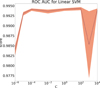 |
Fig. A.1. Dependence of the ROC AUC score with corresponded standard deviation on parameter C for the linear SVM. |
Then, we trained SVM with five-fold cross-validation on SDSS training data. It is worth noting that the cross-validation technique provides the possibility to perform classification on the entire training sample and use the obtained result for validation, as has been done by us for SDSS.
A.3. OCSVM
For OCSVM, with the radial basis function kernel, we were also searching for the optimal free parameters (γ and ν) by simple grid-search using a five-fold cross-validation on the training sample. As a result, we selected the values ν = 10−5 and γ = 10−3, for which the fraction of the off-model objects in the training sample was minimal (only 0.004% objects of the training sample were identified as off-model).
Appendix B: Validation with SDSS and LAMOST
In this section, we describe more detailed validation results obtained by comparing classes of spectroscopically confirmed objects with the predicted ones. We use only the SDSS and LAMOST data since these contain the largest number of stars and galaxies and, therefore, they can represent the entire input of the AllWISE × PS1 catalogue in the best way.
Hereinafter, we designate as “LAMOSTinitial” the initial sample of the AllWISE × PS1 × LAMOST DR4 objects; we define “LAMOSTcleaned” as a subsample of the initial LAMOST sample, in which some objects have passed visual inspection, have resulted in exclusion of some sources from consideration, or had their classes adjusted. We also define “LAMOSTcleaned ⊈ SDSS” as a sample of those objects from LAMOSTcleaned that are not contained in the SDSS catalogue. See Sect. 5.3 for more detailed information about these samples.
B.1. Additional classification quality metrics
We analysed the validation results using several well-known classification quality metrics: purity, completeness, MCC (that are defined in Sect. 5.1), area under receiver operating characteristic curve (ROC AUC), and confusion matrix (see Tables B.1–B.3). We define further the classification metrics that we used.
Classification quality metrics for different validation datasets.
Confusion matrices for validation datasets.
Quality of the classification model within different validation samples.
B.1.1. Confusion matrix
The confusion matrix shows how predictions of object classes are distributed over different classes. Each row of this matrix corresponds to a true class and each column to a predicted one. Then, in classifying objects into stars and extragalactic objects, we would have NSS in the cell of the first column of the first row, NGS in the cell of the first column of the second row, and so on (see Table B.2).
B.1.2. ROC AUC
The receiver operating characteristic (ROC) curve is a visual characteristic that is aimed at demonstrating how confidently the model is able to separate different classes of objects. In practice, to quantitatively estimate the quality of classification, the area under the ROC curve (ROC AUC, Bradley 1997) is used more often. The value of ROC AUC, in the case of ideal classification, is 1.0, while random guessing results in ROC AUC = 0.5.
B.2. Results
The main results for the two validation samples are given in Table B.1 (MCC and ROC AUC), Table B.2 (confusion matrices), and Table B.3 (purity and completeness). As can be seen from Tables B.1 and B.3, the values of parameters MCC, ROC AUC, purity, and completeness of the LAMOSTcleaned significantly improved after a visual inspection of the objects classified as stars in LAMOST, but as galaxies according to our model. As we indicated earlier (see Sect. 5.3), LAMOSTcleaned sample may contain quasars that are labelled as stars in LAMOST, as well as stars that are classified as “extragalactic” in LAMOST. Naturally, the correction of the classes of these objects will improve all indicators of the classification quality.
As a result, only 612/3740 of 1 107 370/306 412 stars (0.05%/1.22% of the sample, see Table B.2) from the LAMOST/SDSS respectively were classified as galaxies. The purity reaches 99.8% for the SDSS, and 98.9% for the LAMOSTcleaned, which we assume as the representative values of classification quality because these values agree with the astrometric test (showing 98.9% of purity up to g ∼ 21.5m). Also, our validation indicates that completeness of the NEWS is approximately 99.2% (with the LAMOST data) and 99.8% (with the SDSS data), which is consistent with the external datasets validation, where completeness is > 99.0% for 19m < g < 22m magnitude range.
We note that quality metrics for the LAMOSTcleaned ⊈ SDSS validation sample are worse than for the LAMOSTcleaned sample (see Table B.3). This is caused by the increasing the class imbalance after removing the sources, common with SDSS, which resulted in decreasing the number of galaxies in three times.
The classification quality on the validation samples (and on the NEWS catalogue, respectively) could be increased, applying W1 < 17m magnitude limit (Krakowski et al. 2016), which results in MCC = 98.00%/99.05% and CG = 98.08%/99.90% for the LAMOSTcleaned ⊈ SDSS and the SDSS samples, respectively. The impact of this limit on the LAMOST sample is negligible due to the small number of sources at the faint end of magnitude range.
Finally, we analysed the dependence of the classification quality on the colour excess E(B − V) (see Fig. B.1). Some regions of the sky with the significant extinction are covered by the SDSS and LAMOST, allowing us to test the classification quality as the function of extinction. As result, the MCC and completeness metrics for the SDSS and LAMOSTcleaned samples are > 98% for E(B − V) < 0.1m; the classification quality degrades starting from E(B − V) = 0.2m for the LAMOST data. This indicates that sky regions with E(B − V)> 0.2m should be discarded from the eventual galaxy catalogue to avoid the relatively high contamination by the stars classified as galaxies in the NEWS.
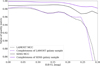 |
Fig. B.1. Dependence of the MCC and completeness on colour excess E(B − V) for LAMOST (dashed lines), and SDSS (solid lines) validation samples. |
All Tables
Number of stars and galaxies in the validation catalogues matched in AllWISE × PS1.
All Figures
|
Fig. 1. Histogram of g magnitude distribution for the AllWISE × PS1 inference (violet) and training (orange) samples of sources. |
| In the text | |
|
Fig. 2. Sky distribution of 40 million objects from the NEWS catalogue in Aitoff projection (galactic coordinates with l = 0°, b = 0° at the centre). |
| In the text | |
|
Fig. 3. Distribution of g − gKron versus g magnitude for 38 million objects. A cut g − gKron = 0.05 (red line) roughly separates the extended objects from the point-like objects. |
| In the text | |
|
Fig. 4. Sky distribution of the pxgal for 40 million sources from the NEWS catalogue in Aitoff projection (galactic coordinates, l = 0°,b = 0° at the centre). |
| In the text | |
|
Fig. 5. Histogram of g magnitude distribution for the validation datasets. |
| In the text | |
|
Fig. 6. Distribution of gPSF − gKron versus W1 − W2 colour for sources that are identified as stars in LAMOST DR4 data, but classified as extragalactic objects within our model. The probability of source being extragalactic pxgal is marked in colour. |
| In the text | |
|
Fig. 7. Distribution of the first two features for the AllWISE × PS1 spectroscopically confirmed sources. Top panel: SDSS training sample; bottom panel: LAMOST validation sample. Left images correspond to the distribution of stars within first two features; right images to the distribution of extragalactic sources. |
| In the text | |
|
Fig. 8. Dependence of the MCC (left) and completeness (right) scores on g magnitude. The coloured lines represent different spectroscopic surveys, which we used to estimate the classification quality metrics. |
| In the text | |
|
Fig. 9. Left: dependence of the components of the rotation vector, ωx, ωy, ωz, of the system, defined by the positions and proper motions of 1.2M NEWS sources with respect to the Gaia-CRF2 on the G magnitude. Right: dependence of components of rotation vector, ωx, ωy, ωz, of the system, defined by the positions and proper motions of 1.0M NEWS sources, passed astrometric criterion, with respect to the Gaia-CRF2 on the G magnitude. Vertical error bars represent the dispersion of components within the magnitude bin. The components ωx, ωz were shifted by ±1.0 mas yr−1 for better visibility. |
| In the text | |
|
Fig. A.1. Dependence of the ROC AUC score with corresponded standard deviation on parameter C for the linear SVM. |
| In the text | |
|
Fig. B.1. Dependence of the MCC and completeness on colour excess E(B − V) for LAMOST (dashed lines), and SDSS (solid lines) validation samples. |
| In the text | |
Current usage metrics show cumulative count of Article Views (full-text article views including HTML views, PDF and ePub downloads, according to the available data) and Abstracts Views on Vision4Press platform.
Data correspond to usage on the plateform after 2015. The current usage metrics is available 48-96 hours after online publication and is updated daily on week days.
Initial download of the metrics may take a while.