© ESO 2020

1. Introduction

Neglecting tides and magnetic braking, Packet (1981) showed that mass gainers continue to rotate with the critical velocity after the accretion of only 5%–10% of their own mass. This critical velocity is in most cases much faster than observed.

Van Rensbergen & De Greve (2008) published results of binary evolutionary computations aimed at reproducing the observed orbital parameters, masses, location in the HRD and rotational velocities of a collection of well-studied Algol-type semi-detached binaries. In this binary evolution code, the effects of mass and angular momentum losses from the system by stellar wind were included, assuming that stellar wind carries the orbital angular momentum of both stars into space. The mass losses by stellar wind were from Vink et al. (2001) for stars hotter than 12 500 K, and De Jager et al. (1988) for cooler stars. In the case of liberal evolution of the system we assumed that the mass-losing gainer carries its specific orbital angular momentum into space.

Our previous work (Van Rensbergen & De Greve 2008) used tidal interaction according to Wellstein (2001). In a subsequent paper, Van Rensbergen & De Greve (2016) included a more refined treatment of tidal interactions. Hereinafter, tides for a star with a radiative atmosphere are very different to those of a star in convection (see e.g. Hilditch 2001). The convective mode was always applied during Roche Lobe Over Flow (henceforth: RLOF). Meridional circulation, as proposed by Tassoul (2000), was added as a significant contributor to the tidal action. This could not, however, explain the observed rotational velocities of the mass gainers published by Van Hamme & Wilson (1990), Miller et al. (2007), Glazunova & Yushcenko (2008) and Dervisoglu et al. (2010).

The influence of magnetic braking on the evolution of binaries has been acknowledged repeatedly in the literature (see e.g. Eggleton & Kiseleva-Eggleton 2002 and Song et al. 2018). Dervisoglu et al. (2010) showed how the rotation of gainers in binaries is braked by assumed magnetic fields of a few kG. Vanbeveren et al. (2018) determined the evolution of the spin of the O components in (WR+O) binaries in a similar way.

The effects of magnetic braking were so far not included in our code. In the present paper, we calculated the magnetic field strength, and hence the magnetic braking, using a simple model of differential rotation. The magnetic fields are variable with time and different for different stars, depending on the evolution of physical parameters at the interface between the inner core and the outer shell of the mass-gaining star. We report the results of magnetic braking included, in order to better understand the observed rotational velocities.

2. Generation of the magnetic field of the gainer

A solid body rotator with constant angular velocity Ω from the centre to the edge of the star cannot develop a magnetic field. For this paper, we used magnetic fields that are produced by the dynamo model of Spruit (2002) which is at work when the angular velocity rises with an amount ΔΩ over a distance Δr. The magnetic field is then directly proportional to the quantity q:

$$\begin{array}{c}\hfill q=\frac{\mathrm{\Delta }\mathrm{\Omega }}{\mathrm{\Omega }}\frac{\mathrm{\Delta }r}{r}.\end{array}$$(1)

In order to calculate q, we used a simplified model to introduce differential rotation into the gainer. We considered the gainer as a star that is composed as a core surrounded by a shell. Before the start of RLOF, both parts rotate synchronously and produce no magnetic field. Magnetic fields can develop from the start of RLOF onwards. The core has a radius R_core and is a rigid rotator with angular velocity Ω_core. The differential rotation of the shell rises from Ω_core at R_core, to Ω_edge at R_g: the physical radius of the gainer. A reasonable evaluation of Ω_edge is hereafter proposed in relation (8). Relation (1) can now be read as:

$$\begin{array}{c}\hfill q=\frac{({\mathrm{\Omega }}_{\mathrm{edge}}-{\mathrm{\Omega }}_{\mathrm{core}})}{{\mathrm{\Omega }}_{\mathrm{core}}}\frac{(R_{\mathrm{g}}-R_{\mathrm{core}})}{R_{\mathrm{core}}}.\end{array}$$(2)

Apart from the evaluation of the quantity q in relation (2), the following quantities needed to compute the magnetic field with the dynamo model of Spruit (2002) are: the Brunt-Väsälä frequency N, the thermal conductivity κ, the magnetic diffusivity η and the density ρ.

These quantities are calculated in the gainer at every stage of the evolution of the binary.

Spruit (2002) calculated the radial component B_r from the azimuthal component B_ϕ of the magnetic field with relations (5) and (6).

The minimum shear rate required for a dynamo to operate is given by the quotient of the magnetic field strength (B) needed to produce the Alfvén frequency divided by the minimum field strength (B_c) for the Tayler instability. These quotients are shown in relations (3) and (4).

If thermal conductivity can be ignored (subscript “0”) one obtains:

$$\begin{array}{c}\hfill \frac{B_0}{B_{c0}}=q{\left(\frac{{\mathrm{\Omega }}_{\mathrm{core}}}{N}\right)}^{\frac{7}{4}}{\left(\frac{R_{\mathrm{core}}^{2}N}{\eta }\right)}^{\frac{1}{4}}<1.\end{array}$$(3)

If this is the case, one includes the thermal conductivity κ in the evaluation and calculates the quotient (subscript “1”):

$$\begin{array}{c}\hfill \frac{B_1}{B_{c1}}=q^{\frac{1}{2}}{\left(\frac{{\mathrm{\Omega }}_{\mathrm{core}}}{N}\right)}^{\frac{7}{8}}{\left(\frac{R_{\mathrm{core}}^{2}N}{\kappa }\right)}^{\frac{1}{8}}{\left(\frac{\kappa }{\eta }\right)}^{\frac{1}{2}}.\end{array}$$(4)

If $\frac{B_1}{B_{c1}}$ > 1, the magnetic field is calculated with relation (6).

We followed this logic. However, when the quotients in relations (3) and (4) are both larger than 1, both modes are able to trigger the working of the dynamo. In that case, the mean value of B_r0 in relation (5) and B_r1 in relation (6) were taken for the magnetic field that governs the magnetic braking:

$$\begin{array}{c}\hfill B_{\varphi 0}=\frac{R_{\mathrm{core}}(4\pi {\rho }^2{)}^{\frac{1}{2}}q{\mathrm{\Omega }}_{\mathrm{core}}^2}{N};\frac{B_{r0}}{B_{\varphi 0}}=q{\left(\frac{{\mathrm{\Omega }}_{\mathrm{core}}}{N}\right)}^2\end{array}$$(5)

$$\begin{array}{c}\hfill \begin{array}{c}\hfill B_{\varphi 1}=R_{\mathrm{core}}(4\pi {\rho }^2{)}^{\frac{1}{2}}{q}^{\frac{1}{2}}{\mathrm{\Omega }}_{\mathrm{core}}{\left(\frac{{\mathrm{\Omega }}_{\mathrm{core}}}{N}\right)}^{\frac{1}{8}}{\left(\frac{\kappa }{N{R}_{\mathrm{core}}^2}\right)}^{\frac{1}{8}};\\ \hfill \frac{B_{r1}}{B_{\varphi 1}}={\left(\frac{{\mathrm{\Omega }}_{\mathrm{core}}}{N}\right)}^{\frac{1}{4}}{\left(\frac{\kappa }{N{R}_{\mathrm{core}}^2}\right)}^{\frac{1}{4}}.\end{array}\end{array}$$(6)

The values of ρ, κ, N, and η in relations (3)–(6) are evaluated at the interface between the core and the shell.

From the start of RLOF onwards, the core of the gainer is not influenced by the matter coming from the donor and impinging on the surface of the gainer. The amount of angular momentum that is added only to the shell is given by Packet (1981), reduced by the quotient of the impact-parameter d over the radius of the gainer R_g, rendering the spin-up inefficient at close approach:

$$\begin{array}{c}\hfill \mathrm{\Delta }{J}_{\mathrm{spin},\mathrm{shell}}^{+}=6.04534\times {10}^{54}{R}_{\mathrm{g}}{(M_{\mathrm{g}}+\frac{\mathrm{\Delta }{M}_{\mathrm{g}}}{2})}^{\frac{1}{2}}\left(\frac{d}{R_{\mathrm{g}}}\right).\end{array}$$(7)

$\mathrm{\Delta }{J}_{\text{spin},\text{shell}}^{+}$ is expressed in cgs units, whereas masses and radii are, respectively, in M_⊙ and R_⊙.

With every value of J_{spin, shell} corresponds a value of Ω_shell = J_{spin, shell}/I_shell, which is a characteristic value of the angular velocity in the shell. A magnetic field is created when Ω_shell  >   Ω_core. The value of Ω cannot, however, change discontinuously from Ω_core to Ω_shell at the interface between core and shell.

In order to accomplish the continuity of Ω(r) and to avoid friction between the outer edge of the core and the inner surface of the shell, we chose a radius-dependent angular velocity Ω(r) raising continuously from Ω_core at the interface between core and shell to Ω_edge at the edge of the gainer. Although any other choice would have been possible, we assumed that this growth follows the shape of an ellipse, somewhat similar to the shape of the tacholine in the sun as used by Spruit (2002) to explain the observed general magnetic field of the sun (B_r about 1 Gauss).

Requiring that the amount of angular momentum in the shell remains the same as for a rigidly rotating shell with uniform angular velocity Ω_shell, one obtains:

$$\begin{array}{c}\hfill {\mathrm{\Omega }}_{\mathrm{edge}}=\frac{4}{\pi }({\mathrm{\Omega }}_{\mathrm{shell}}-{\mathrm{\Omega }}_{\mathrm{core}})+{\mathrm{\Omega }}_{\mathrm{core}}.\end{array}$$(8)

3. Evolution of a binary including magnetic braking

3.1. Conservation of angular momentum

The total angular momentum J_Σ of a binary is the sum of the orbital angular momentum J_orb and the spin angular momenta of gainer J_g and donor J_d. Tides continuously exchange amounts of ΔJ_orb, ΔJ_g and ΔJ_d. In the conservative case, one obtains:

$$\begin{array}{c}\hfill \mathrm{\Delta }{J}_{\mathrm{\Sigma }}=\mathrm{\Delta }{J}_{\mathrm{orb}}+\mathrm{\Delta }{J}_{\mathrm{g}}+\mathrm{\Delta }{J}_d=0.\end{array}$$(9)

Angular momentum loss due to stellar wind (SW), mass loss from the system during liberal eras of RLOF (OUT) and angular momentum loss due to magnetic braking (MAG) do not violate the law of conservation of angular momentum, but change the angular momentum balance into:

$$\begin{array}{c}\hfill \mathrm{\Delta }{J}_{\mathrm{orb}}+\mathrm{\Delta }{J}_{\mathrm{g}}+\mathrm{\Delta }{J}_d-\mathrm{\Delta }{J}_{d+\mathrm{g}}^{\mathrm{SW}+\mathrm{OUT}}-\mathrm{\Delta }{J}_{\mathrm{g}}^{\mathrm{MAG}}=0.\end{array}$$(10)

The values of $\mathrm{\Delta }{J}_{d+\text{g}}^{\text{SW+OUT}}$ and $\mathrm{\Delta }{J}_{\text{g}}^{\text{MAG}}$ are negative. The amount of angular momentum $\mathrm{\Delta }{J}_{\text{g}}^{\text{MAG}}$ has only been lost by the gainer’s shell.

Since the core rotates as a solid body, no magnetic field (and hence no magnetic braking) is created in the core.

In this paper, we emphasise the effect of magnetic braking, since this was not included in our previous papers. The amount of angular momentum lost by the gainer’s shell due to magnetic braking is given by Dervisoglu et al. (2010) in cgs units:

$$\begin{array}{c}\hfill \mathrm{\Delta }{J}_{\mathrm{g}}^{\mathrm{MAG}}=-(4.807043\times {10}^{40}{\left(\frac{\mathrm{d}M}{\mathrm{d}t}\right)}^{\frac{3}{7}}{\left(R\right)}^{\frac{24}{7}}{\left(B\right)}^{\frac{8}{7}}{\left(M\right)}^{\frac{-2}{7}}{\mathrm{\Omega }}_{\mathrm{edge}}\mathrm{\Delta }t).\end{array}$$(11)

Here, the quantity B is the radial component of the magnetic field produced by the dynamo model of Spruit (2002) expressed in Gauss. The quantity $\frac{\mathrm{d}M}{\mathrm{d}t}$ is the stellar wind mass loss of the gainer in $\frac{M_{\odot }}{\mathrm{year}}$. This wind carries matter and angular momentum into space. Furthermore, R is the radius of the gainer in R_⊙, M is the mass of the gainer expressed in M_⊙ and Ω_edge is the angular velocity at the edge of the gainer, defined in relation (8). So, v_eq, g = Ω_edgeR_eq, g.

Relation (11) is the expression derived by Dervisoglu et al. (2010) for a magnetic dipole, which is valid in this case.

3.2. Calculating the orbital period

The orbital angular momentum was calculated from relation (10). From this value the orbital period is calculated for circular orbits in cgs units with:

$$\begin{array}{c}\hfill J_{\mathrm{orb}}=1.045064\times {10}^{51}{P}^{\frac{1}{3}}\frac{M_d{M}_{\mathrm{g}}}{{(M_d+M_{\mathrm{g}})}^{\frac{1}{3}}}.\end{array}$$(12)

The orbital period P is in days and the masses in M_⊙.

3.3. Extent of the shell applied to the evolution of a progenitor of λ Tau

The gainer is now composed of an inner core in solid rotation surrounded by a shell that rotates differentially. The core is not spun up nor slowed down magnetically. Its rotation is only modulated by tides. The shell is spun up following relation (7). Its rotation is modulated by tides and undergoes magnetic braking following relation (11).

A core that takes a core fraction CF of the total mass of the gainer leaves (1-CF) of the mass for the shell.

Figure 1 shows the evolution with time of the equatorial velocity of the gainer starting from a (6.36 + 2,7) M_⊙ binary with an initial orbital period of 1.89745 d. This is a plausible progenitor for λ Tau. The calculation was performed for the system undergoing tides and magnetic braking with initial value of CF = 0.95. This evolution with time is compared with the evolution of the gainer in the same system with a rigidly rotating and hence never magnetic gainer for which the rotation is affected by tides only. The evolution towards the point when neither tides nor magnetic braking are active is also included in the figure, which shows then a gainer rotating continuously with critical velocity once this velocity is achieved.

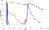Fig. 1. Evolution with age (in years) of the equatorial velocity (in km s−1) of the gainer of a (6.36 M⊙ + 2.7 M⊙) binary with an initial period of 1.89745 days. A likely progenitor of λ Tau. With the black line, tides and magnetic braking are not at work. With the red line tides act alone. With the blue line tides and magnetic braking act together.

The plausible progenitor for λ Tau starts RLOF during core hydrogen burning of the donor. Critical rotation of the gainer is achieved during a phase of rapid RLOF at around 48 million years after ZAMS. After that, RLOF occurs at a lower speed. Tidal interaction and magnetic braking are then strong enough to synchronize the rotation of the gainer. In Figure 1 one sees clearly that synchronization settles more rapidly when magnetic braking helps tidal interaction. After around 65 million years, during the hydrogen shell burning of the donor, RLOF restarts. Critical rotation is again attained. But the rush to critical rotation is slowed down by the combined action of tides and magnetic braking. The present observed state of λ Tau occurs during this stage of rising rotational velocity. The gainer of λ Tau now has an equatorial velocity of 178 km s⁻¹, far below the critical value of 552 km s⁻¹.

When critical rotation is achieved during RLOF B the orbital period is about 30 days. Figure 1 shows that tides are then too weak to prevent critical rotation. Magnetic braking will, however, decrease the velocity below the critical value. This work is done at the very end of, and after, RLOF B.

Figure 2 shows the evolution of the magnetic field of the gainer in the binary shown in Fig. 1. The magnetic field is generated by the difference of angular velocity Ω between the shell and core. Before RLOF A, the shell and core of the gainer have the same synchronous rotational velocity. The core always continues to rotate almost synchronously. When RLOF A starts, only the shell is spun up. When the shell rotates at critical velocity, the magnetic field is at a maximum of approximately 3000 Gauss. When tides and magnetic braking have synchronised the rotation of the shell, the magnetic field disappears. From the beginning of RLOF B, the shell is again spun-up, and the magnetic field starts to be built up again. The value of the magnetic field is lower than during rapid RLOF A. A value of about 750 Gauss is reached. Since magnetic braking is then nevertheless very active, the shell is gradually synchronised. After that, the magnetic field disappears again.

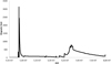Fig. 2. Evolution of the magnetic field strength (in Gauss) produced by the Spruit mechanism for the binary mentioned in Fig. 1.

In summary, the magnetic field is large at high equatorial velocities (large ΔΩ) and small at low equatorial velocities (small ΔΩ). Figure 2 shows the eras where the gainer can be considered as a magnetic star.

A progenitor is plausible when the calculated positions of donor and gainer in the HRD are found to be close to the observations. Figure 3 shows the evolutionary path of the plausible progenitor of λ Tau for which the evolution of the equatorial velocity and of the magnetic field strength of the gainer are shown in Figs. 1 and 2.

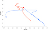Fig. 3. Evolution through the HRD of the binary taken as an example in Figs. 1 and 2. The donor follows the blue path and its current observed position is a triangle, whereas the observed rejuvenated gainer follows the red path and its current position is a filled circle.

Calculations show that choices different from an initial value of CF = 0.95 (5% of the mass of the gainer in the shell), would hardly change the results shown in Figs. 1 and 2. Only an initial value of CF = 0 is of course not justified, because this option produces a solid rotator in which no magnetic field is produced.

Figure 4 shows the evolution of the quantity CF for the gainer of the binary shown in Figs. 1–3. The gainer has an initial mass of 2.7 M_⊙. With CF = 0.95 one has a shell with an initial mass of 0.135 M_⊙. The solidly rotating core keeps its mass of 2.565 M_⊙ during the entire evolution. At the end of RLOF A, the mass of the gainer has grown up to 6.936 M_⊙. Since the core maintains its initial mass, the mass of the shell raises up to 4.371 M_⊙, containing 63% of the gainer’s mass (CF = 0.37). At the end of RLOF B, the mass of the gainer is again somewhat larger and the value of CF shrinks to 0.31.

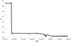Fig. 4. Mass fraction of the core (CF) decreases with time during the evolution of the system shown in Figs. 1–3.

This is not so different from the evolution of a shell with, for example, an initial value of CF = 0.5 that ultimately evolves into a massive shell with CF = 0.2 (80% of the mass of the gainer being in the shell), giving rise to magnetic fields and magnetic braking that are very similar to those obtained with an initial value of CF = 0.95. This value was used in all our calculations.

3.4. Calculated cases

We found 44 binaries for which the equatorial velocity of the gainer was published. These systems are shown in Tables 1 and 2.

For every binary in these tables, we calculated the evolution of a number of possible progenitors. In the case of conservative evolution, the initial orbital period P₀ of every progenitor was determined from the presently observed period P₁ with relation (13), which obeys to the rule of conservation of angular momentum:

$$\begin{array}{c}\hfill \frac{P_0}{P_1}={\left(\frac{M_{d,1}\times M_{\mathrm{g},1}}{M_{d,0}\times M_{\mathrm{g},0}}\right)}^3.\end{array}$$(13)

The subscript d is for the donor and g for the gainer. Although we calculated the orbital period with relations (10)–(12) using our code, relation (13) yields correct initial periods in the case of conservative evolution. This demonstrates that neglecting the spin angular momenta of the individual stars, as done in relation (13), is of minor importance.

In the case of liberal evolution initial periods are determined with relation (14). This relation is valid when all matter that leaves the system takes only the orbital angular momentum of the involved stars.

$$\begin{array}{c}\hfill \frac{P_0}{P_1}={\left(\frac{M_{d,1}\times M_{\mathrm{g},1}}{M_{d,0}\times M_{\mathrm{g},0}}\right)}^3\times {\left(\frac{M_1}{M_0}\right)}^2.\end{array}$$(14)

Here, M is the total mass of the system, so that:

$$\begin{array}{c}\hfill M_1=M_0-|\mathrm{\Delta }{M}^{\mathrm{SW}}|-|\mathrm{\Delta }{M}^{\mathrm{OUT}}|.\end{array}$$(15)

The quantity ΔM^SW, the amount of mass that leaves the system as stellar wind, is always small compared to the stellar masses. The quantity ΔM^OUT is the amount of RLOF mass that is not accreted by the gainer. This amount can be large and is difficult to predict. In our sample of 44 binaries, only two of them (V356 Sgr and TU Mon) experienced a liberal era during their life. The calculated masses of their components correspond less well to the observed values when compared to the cases with conservative evolution. For the liberal evolutions, relation (14) turns out to give less reliable initial periods, except in the case that the assumed value of ΔM^OUT proves to have exactly the same value as calculated by our code.

When the initial period is sufficiently large, RLOF A, as shown in Sect. 3.3 for a plausible progenitor of λ Tau, is skipped from the evolution. The first RLOF starts then during hydrogen shell burning of the donor. In this case, calculations show that it is more difficult to avoid critical rotation.

4. Results and future work

Van Hamme & Wilson (1990) defined the quantities $F=\frac{v_{\mathrm{eq}}}{v_{\mathrm{sync}}}$ and $R=\frac{F_{\mathrm{gainer}}-1}{F_{\mathrm{crit},\mathrm{gainer}}-1}$. In this case, R ∈ [0–1] is a measure of rotation. Specifically, R is 0 at synchronous rotation and 1 at critical rotation. The use of the quantity R as a characteristic measure of rotation has the advantage that minor differences in the evaluation of the synchronous and critical velocities by different authors are ironed out.

Tables 1 and 2 compare the masses of the components and the equatorial velocity characteristics of the gainers as obtained by our code with the observations. For every system a consistent number of possible progenitors was calculated from birth to the moment that the gainer leaves the main sequence. The initial periods were calculated with relation (13) or (14). From the many possible progenitors only the most plausible were included in the tables. For a few systems two plausible progenitors are mentioned. The calculated numbers are taken at the presently observed orbital period. The ranking runs from perfect determination to bad determination of v_eq from the top of Table 1 to the bottom of Table 2. A determination of v_eq is considered to be good when ΔR = |R_model − R_obs| is small (near to 0) and is unacceptable when the same quantity is large (near to 1).

The results and reservations about the tables are:

– Results are shown in Tables 1 and 2 for 44 binaries.

– The observed equatorial velocities of 16 systems are very well confirmed by theory (ΔR <  0.1).

– 17 more systems can be considered as well explained by the theory (ΔR∈ [0.11–0.35]).

– Eight more systems are weakly reproduced by theory (ΔR∈ [0.50–0.90]).

– Only three systems are poorly reproduced with the theory (ΔR >  0.90). The observed equatorial velocities are far below critical in these cases. However, model calculations from all possible progenitors result in critical rotators. What they have in common is that the calculated models appear to be in the phase of rapid RLOF at the current observed period, when up-spinning cannot be slowed down by the combined action of tides and magnetic braking. In that case, our model fails to explain the observed spin characteristics of the binary.

– Poorly explained cases are shown at the bottom of Table 2.

– Braking of rapidly rotating gainers can be strengthened by the action of a magnetic torque. We invite the reader to consult, for example Tout & Pringle (1992) who spun-down rapidly rotating convective single stars with a magnetic torque due to the interaction with their accretion disc. Martin et al. (2011) used decretion discs for the down-spinning of B_e stars. Wickramasinghe et al. (2014) dissipated the differential rotation into rigid rotation of a recently formed star resulting from the merging of two protostars into a star that owes its magnetic field to its differential rotation that has disappeared in the mean time. These examples cannot be simply applied to the gainer in a binary that evolves in a very different way. Additionally, RLOF will maintain differential rotation in the shell of the gainer. Nevertheless, the exchange of angular momentum between the (in our simple model) fast differentially rotating magnetic shell and the slower rigidly rotating non-magnetic core can reduce the value of the equatorial velocity of the gainer, and this will be included in our future research.

– Current orbital periods are well known. This is, however, less so the case for current stellar masses. It is therefore not impossible that some observed stellar masses need to be revised. In that case, they have to be approached with a different set of possible progenitors, (perhaps) yielding “better” results.

– Observed values of equatorial velocities below synchronous velocity are usually not reproduced by our calculations since tides always tend to synchronize the rotation.

5. Conclusions

For systems with small initial orbital periods, our models predict two stages with strong magnetic fields. The first one occurs during phase A of RLOF at a high mass-transfer rate and lasts rather a short period of time, In the example discussed in Sect. 3.3 the mass transfer rate goes up to (5 × 10⁻⁵) $\left(\frac{M_{\odot }}{\mathrm{yr}}\right)$, and the duration of a large magnetic field (above 1 kG with a maximum of 3 kG) lasts for 3 × 10⁵ years. At that stage, the spectral lines are heavily rotationally broadened by the critical rotation.

The second stage, during phase B of RLOF, lasts longer during a period of lower mass-transfer. However, the mass transfer rate goes up to 10⁻⁶ $\frac{M_{\odot }}{\mathrm{yr}}$ and the duration of a large magnetic field lasts for 10⁷ years. This magnetic field strength is less high compared to the one that is active during RLOF A and shrinks from a maximum of 750–100 Gauss. Then, the spectral lines then are again rotationally broadened due to the critical rotation of the gainer.

The detection of Zeeman effect at work in the spectra of gainers rotating at large equatorial velocities might be problematic. But it would offer a test for the validity of our model.

For systems with larger initial orbital periods RLOF A will be skipped from the evolution. Straight RLOF B will spin the gainer up, more or less quickly, to critical velocity. This critical velocity remains until the end of RLOF B. At that moment, the orbital period is large and critical velocities cannot be dragged below this limit by weak tidal interaction. Magnetic braking will be the major mechanism that will ultimately synchronize the gainer.

Despite the fact that we used a simple model for differential rotation of the gainer in order to generate magnetic braking, we found that 75% of the observed rotational velocities of gainers in interacting binaries were reproduced reasonably well by our model. In less than 10% of the examined cases, our model failed completely to reproduce the observations. This might show that our model is not applicable in these cases, but also that observers could evaluate new values for equatorial velocities of gainers and masses of the components in interacting binaries. Different masses indeed yield different sets of possible progenitors that reproduce the characteristics of the current binary. On the other hand the observed orbital periods are correctly listed.

Researchers who want to obtain calculations with our current binary evolutionary code are welcome to request this from us.

Acknowledgments

We thank Henk Spruit for explaining patiently how his dynamo works. We thank the referee and Edward Van den Heuvel for their constructive and helpful comments.

References

All Tables

All Figures

	Fig. 1. Evolution with age (in years) of the equatorial velocity (in km s−1) of the gainer of a (6.36 M⊙ + 2.7 M⊙) binary with an initial period of 1.89745 days. A likely progenitor of λ Tau. With the black line, tides and magnetic braking are not at work. With the red line tides act alone. With the blue line tides and magnetic braking act together.
In the text

	Fig. 2. Evolution of the magnetic field strength (in Gauss) produced by the Spruit mechanism for the binary mentioned in Fig. 1.
In the text

	Fig. 3. Evolution through the HRD of the binary taken as an example in Figs. 1 and 2. The donor follows the blue path and its current observed position is a triangle, whereas the observed rejuvenated gainer follows the red path and its current position is a filled circle.
In the text

	Fig. 4. Mass fraction of the core (CF) decreases with time during the evolution of the system shown in Figs. 1–3.
In the text

References

- Brancewicz, H., & Dworak, T. 1980, Acta Astron., 30, 501 [Google Scholar]
- Budding, E., Erdem, A., Cicek, C., et al. 2004, A&A, 417, 263 [NASA ADS] [CrossRef] [EDP Sciences] [Google Scholar]
- De Jager, C., Nieuwenhuyzen, H., & Van der Hucht, K. 1988, A&AS, 72, 259 [Google Scholar]
- Dervisoglu, A., Tout, C., & Ibanglu, C. 2010, MNRAS, 406, 1071 [Google Scholar]
- Dominis, D., Mimica, P., Pavlovski, K., & Tamajo, E. 2005, ApSS, 296, 189 [Google Scholar]
- Eggleton, P., & Kiseleva-Eggleton, L. 2002, ApJ, 575, 461 [NASA ADS] [CrossRef] [Google Scholar]
- Glazunova, L., & Yushcenko, A. 2008, AJ, 135, 1736 [NASA ADS] [CrossRef] [Google Scholar]
- Hilditch, R. 2001, An Introduction to Close Binary Stars (Cambridge University Press) [CrossRef] [Google Scholar]
- Martin, R., Pringle, J., Tout, C., & Lubow, H. 2011, MNRAS, 416, 2827 [NASA ADS] [CrossRef] [Google Scholar]
- Miller, B., Budaj, J., & Richards, M. 2007, ApJ, 656, 1075 [NASA ADS] [CrossRef] [Google Scholar]
- Packet, P. 1981, A&A, 102, 17 [Google Scholar]
- Song, H., Meynet, G., Maeder, A., Ekström, S., et al. 2018, A&AS, 609, A3 [NASA ADS] [CrossRef] [EDP Sciences] [Google Scholar]
- Spruit, H. R. 2002, A&A, 381, 923 [NASA ADS] [CrossRef] [EDP Sciences] [Google Scholar]
- Tassoul, J. L., 2000, Stellar Rotation (Cambridge University Press) [CrossRef] [Google Scholar]
- Tout, C., & Pringle, J. 1992, MNRAS, 256, 269 [CrossRef] [Google Scholar]
- Vanbeveren, D., Mennekens, N., Shara, M., & Moffat, A. 2018, A&A, 615, A65 [NASA ADS] [CrossRef] [EDP Sciences] [Google Scholar]
- Van Hamme, W., & Wilson, R. 1990, AJ, 100, 1982 [NASA ADS] [CrossRef] [Google Scholar]
- Van Rensbergen, W., & De Greve, J. P. 2016, A&A, 592, A151 [NASA ADS] [CrossRef] [EDP Sciences] [Google Scholar]
- Van Rensbergen, W., De Greve, J. P., et al. 2008, A&A, 487, 1129 Vizier Online Data Catalog: J/A&A/487/1129 [NASA ADS] [CrossRef] [EDP Sciences] [Google Scholar]
- Van Rensbergen, W., De Greve, J. P., Mennekens, N., et al. 2010, A&A, 510, A13 [NASA ADS] [CrossRef] [EDP Sciences] [Google Scholar]
- Van Rensbergen, W., De Greve, J. P., Mennekens, N., et al. 2011, A&A, 528, A16 [NASA ADS] [CrossRef] [EDP Sciences] [Google Scholar]
- Vink, J., De Koter, A., & Lamers, H. 2001, A&A, 369, 574 [NASA ADS] [CrossRef] [EDP Sciences] [Google Scholar]
- Wellstein, S. 2001, PhD Thesis, Potsdam University [Google Scholar]
- Wickramasinghe, D., Tout, C., & Ferrario, L. 2014, MNRAS, 437, 675 [NASA ADS] [CrossRef] [Google Scholar]