| Issue |
A&A
Volume 642, October 2020
|
|
|---|---|---|
| Article Number | A118 | |
| Number of page(s) | 21 | |
| Section | Extragalactic astronomy | |
| DOI | https://doi.org/10.1051/0004-6361/202037847 | |
| Published online | 12 October 2020 | |
The magnetized disk-halo transition region of M 51⋆
1
Max-Planck-Institut für Radioastronomie, Auf dem Hügel 69, 53121 Bonn, Germany
e-mail: This email address is being protected from spambots. You need JavaScript enabled to view it.
2
Fakultät für Physik, Universität Bielefeld, Postfach 100131, 33501 Bielefeld, Germany
3
School of Mathematics, Statistics and Physics, Herschel Building, Newcastle University, Newcastle-upon-Tyne NE1 7RU, UK
4
Dept. of Space, Earth and Environment, Chalmers University of Technology, Onsala Space Observatory, 439 92 Onsala, Sweden
5
School of Astronomy, Institute for Research in Fundamental Sciences, PO Box 19395-5531, Tehran, Iran
6
National Radio Astronomy Observatory, 1003 Lopezville Road, Socorro, NM 87801, USA
7
Department of Astrophysics/IMAPP, Radboud University Nijmegen, PO Box 9010, 6500 GL Nijmegen, The Netherlands
Received:
28
February
2020
Accepted:
24
June
2020
Abstract
The grand-design face-on spiral galaxy M 51 is an excellent laboratory for studying magnetic fields in galaxies. Due to wavelength-dependent Faraday depolarization, linearly polarized synchrotron emission at different radio frequencies yields a picture of the galaxy at different depths: observations in the L-band (1–2 GHz) probe the halo region, while at 4.85 GHz (C-band) and 8.35 GHz (X-band), the linearly polarized emission mostly emerges from the disk region of M 51. We present new observations of M 51 using the Karl G. Jansky Very Large Array at the intermediate frequency range of the S-band (2–4 GHz), where previously no high-resolution broadband polarization observations existed, to shed new light on the transition region between the disk and the halo. We present the S-band radio images of the distributions of the total intensity, polarized intensity, degree of polarization, and rotation measure (RM). The RM distribution in the S-band shows a fluctuating pattern without any apparent large-scale structure. We discuss a model of the depolarization of synchrotron radiation in a multi-layer magneto-ionic medium and compare the model predictions to the multi-frequency polarization data of M 51 between 1–8 GHz. The model makes distinct predictions of a two-layer (disk–halo) and three-layer (far-side halo “disk” near-side halo) system. Since the model predictions strongly differ within the wavelength range of the S-band, the new S-band data are essential for distinguishing between the different systems. A two-layer model of M 51 is preferred. The parameters of the model are adjusted to fit to the data of polarization fractions in a few selected regions. In three spiral arm regions, the turbulent field in the disk dominates with strengths between 18 μG and 24 μG, while the regular field strengths are 8 − 16 μG. In one inter-arm region, the regular field strength of 18 μG exceeds that of the turbulent field of 11 μG. The regular field strengths in the halo are 3 − 5 μG. The observed RMs in the disk-halo transition region are probably dominated by tangled regular fields, as predicted from models of evolving dynamos, and/or vertical fields, as predicted from numerical simulations of Parker instabilities or galactic winds. Both types of magnetic fields have frequent reversals on scales similar to or larger than the beam size (∼550 pc) that contribute to an increase of the RM dispersion and to distortions of any large-scale pattern of the regular field. Our study devises new ways of analyzing and interpreting broadband multi-frequency polarization data that will be applicable to future data from, for example, the Square Kilometre Array.
Key words: galaxies: general / galaxies: magnetic fields / galaxies: individual: M 51 / galaxies: ISM
The reduced FITS images of this paper are only available at the CDS via anonymous ftp to cdsarc.u-strasbg.fr (130.79.128.5) or via http://cdsarc.u-strasbg.fr/viz-bin/cat/J/A+A/642/A118
© M. Kierdorf et al. 2020
 Open Access article, published by EDP Sciences, under the terms of the Creative Commons Attribution License (https://creativecommons.org/licenses/by/4.0), which permits unrestricted use, distribution, and reproduction in any medium, provided the original work is properly cited.
Open Access funding provided by Max Planck Society.
1. Introduction
Magnetic fields play an important role in the formation and evolution of spiral galaxies (e.g., Wang & Abel 2009; Pillepich et al. 2018; Berlok & Pfrommer 2019), but knowledge of their structure, strength, and origin remains limited. Large-scale patterns of ordered magnetic fields have been observed in multiple nearby spiral galaxies. In face-on galaxies the magnetic field structure shows a spiral pattern, usually following the gaseous spiral arms (e.g., Beck 2016; Beck & Wielebinski 2013). In edge-on galaxies, magnetic fields in the disk are observed mostly parallel to the disk plane, while vertical components are found in the halo (e.g., Haverkorn & Heesen 2012; Wiegert et al. 2015; Krause 2019; Krause et al. 2020).
The exchange of material between disk and halo seems to be a crucial process in the evolution of spiral galaxies. The interaction is believed to be driven by gas flows from so-called galactic fountains (e.g., Shapiro & Field 1976; Bregman 1980). Large-scale halo fields could result from advection of disk fields into the halo, for example, via winds (e.g., Breitschwerdt et al. 1991; Elstner et al. 1995; Pakmor et al. 2018; Steinwandel et al. 2020), or from a dynamo operating in the halo (Sokoloff & Shukurov 1990; Moss et al. 2010; Braun et al. 2010). Due to the lack of simultaneous measurements of both disk and halo field structures in galaxies, the origin of large-scale halo fields and how they are connected to the underlying galactic disk remains poorly understood.
Radio polarization observations are ideal to study the structure of magnetic fields in the interstellar medium (ISM) of spiral galaxies. Synchrotron emission traces the magnetic field component B⊥ in the plane of the sky, perpendicular to the line-of-sight. To obtain a three-dimensional picture of the magnetic field, the effect of Faraday rotation can be used to infer the magnetic field component along the line-of-sight, B∥. The plane of polarization of an electromagnetic wave is rotated when the wave passes through a magnetized plasma containing thermal electrons:
 (1)
(1)
where ψ is the measured polarization angle at wavelength λ, ψ0 is the polarization angle of the emitted electromagnetic wave, and RM is the rotation measure. RM is related to the Faraday depth Φ, a physical quantity dependent on the line-of-sight integral of the thermal electron density, ne, times the magnetic field component along the line-of-sight, B∥:
 (2)
(2)
where dL denotes the infinitesimal path length through the Faraday-rotating medium. By convention, Φ is positive (negative) for magnetic fields pointing towards (away from) the observer. For a simple Faraday-rotating screen located between the synchrotron-emitting source and the observer, RM is equivalent to Φ. There are, however, more complicated cases (e.g., O’Sullivan et al. 2012; Anderson et al. 2016; Ma et al. 2019), such as several mixed synchrotron-emitting and Faraday-rotating media located within the volume traced by the telescope beam.
The degree of polarization, p, given by the ratio of the polarized intensity to the total intensity of the synchrotron emission, is a measure of the degree of order of the magnetic field. The observed degree of polarization can be attenuated by depolarization mechanisms: (1) beam depolarization decreases the polarized signal due to tangled magnetic fields on scales smaller than one resolution element of the observing instrument; (2) in bandwidth depolarization, the plane of polarization is rotated by different angles at different frequencies within the observing frequency band. Averaging over the frequency band entails the reduction of the polarized signal; (3) and by wavelength-dependent depolarization due to Faraday rotation intrinsic to the source and/or along the line-of-sight. One differentiates between differential Faraday rotation and external and internal Faraday dispersion (Sokoloff et al. 1998). With broadband polarization data, wavelength-dependent Faraday depolarization can be used as a powerful probe of the 3D structure of magnetic fields in galaxies (“Faraday tomography”).
The grand-design face-on spiral galaxy M 51 provides an excellent laboratory to simultaneously probe its disk and halo1 fields using wideband polarimetry. Polarization studies of M 51 have shown that different configurations of the large-scale regular magnetic field exist in the disk (probed by observations at 4.85 and 8.35 GHz, Berkhuijsen et al. 1997; Fletcher et al. 2011) and in the halo (probed by observations at 1 GHz, e.g., Horellou et al. 1992; Neininger et al. 1996; Mao et al. 2015). According to Fletcher et al. (2011), the large-scale regular field in the disk is best described by a superposition of two azimuthal modes (axisymmetric plus quadrisymmetric, m = 0 and 2), whereas the halo field has a strong bisymmetric azimuthal mode (m = 1). This difference in the magnetic field configurations in the disk and the halo of M 51 is still an unresolved mystery.
Fletcher et al. (2011) suggested that interactions with M 51’s companion galaxy NGC 5195 could be responsible for the configuration in the halo by driving a different mean-field α–Ω dynamo, for example, through tidal forces. Another possibility is that the halo field could have been generated during early evolutionary stages of M 51 in the disk and later transported into the halo, while a different dynamo action built the present-day disk field. Independent dynamo action in disk and halo of the same galaxy is possible, under the condition that the disk and halo fields are generated by a mean-field α–Ω dynamo that is based on differential rotation and turbulence (Sokoloff & Shukurov 1990). However, Moss et al. (2010) argued that in the presence of a galactic wind the halo component of the field may “enslave” that of the disk, making different field patterns improbable.
A better understanding of M 51’s mysterious magnetic field configuration in the disk and halo and the underlying dynamo mechanism(s) will come from observations of the transition region, which are provided by observations at an intermediate frequency range. Our new broadband S-band polarization data fill the frequency gap between data obtained by the Karl G. Jansky Very Large Array (VLA) at the L-band (1–2 GHz) by Mao et al. (2015) probing the halo, and the C-band (4.85 GHz) and the X-band (8.35 GHz) data (VLA + Effelsberg) by Fletcher et al. (2011) probing mostly the disk. With the combined high quality and broad frequency coverage dataset we are able to investigate the magneto-ionic properties in different layers of M 51.
One of the main motivations of this work was to compare the observed degree of synchrotron polarization in the S-band to an analytical multi-layer depolarization model with different magnetic field configurations developed by Shneider et al. (2014a). This model is more advantageous compared to “classical” depolarization models, which only handle depolarization in a single-layer system (e.g., O’Sullivan et al. 2012; Anderson et al. 2016). Shneider et al. (2014a) modeled the degree of polarization as a function of wavelength assuming different magnetic field configurations to be present in different layers along the line-of-sight in terms of regular, isotropic turbulent, and anisotropic turbulent fields (for a detailed description of the nomenclature please see Beck et al. 2019). Since the model predictions strongly differ within the wavelength range of the S-band, our new data are crucial to evaluate whether the model predictions are adequate.
We present new Karl G. Jansky VLA S-band observations of M 51 in total and polarized intensity. In Sect. 2, we present details of the observations and data reduction. Section 3.1 gives an overview on the total intensity results. In Sect. 4, we summarize the results of polarization analysis (we present maps of polarized intensity, degree of polarization, and rotation measure). In Sect. 5, we compare the observed degree of polarization across a frequency range of 1–8 GHz (a wavelength range of λ3–30 cm) to the Shneider et al. (2014a) model. In Sect. 6, we discuss our main physical findings, while Sect. 7 summarizes the paper including an overview on future prospects. Most of the material contained in this paper was published in a PhD thesis at the University of Bonn (Kierdorf 2019). Preliminary results were published in Kierdorf et al. (2018).
We adopt a distance to M 51 of 7.6 Mpc (Ciardullo et al. 2002), an inclination of the disk of l = −20° (0° is face-on), and a position angle of the disk’s major axis of PA = −10° (Tully 1974).
2. Observations and data reduction
The observations in the S-band (2–4 GHz) were performed using the VLA operated by the National Radio Astronomy Observatory (NRAO) in New Mexico, USA. The observations were done in C- and D-array configuration in November and December 2014, and in October 2015. We observed M 51 in full polarization, while the sources J1313+5458 and J1407+2827 (assumed to be unpolarized) were observed for phase and polarization leakage calibration, respectively. The calibrator 3C 286 was used as the total flux density scale and polarization angle calibrator (Perley & Butler 2013a,b) with a polarization angle of +33° across the S-band. The measurement sets contain 16 spectral windows, each with 64 2 MHz channels. M 51 was observed two times 90 min in C-configuration and 90 min in D-configuration to fill the missing spacings in the C-configuration data. The resolution of the concatenated observations is 10″ × 7″ at 3 GHz (using robust weighting). At the assumed distance of M 51, 1″ corresponds to a linear scale of about 37 pc. Therefore, one beam of 10″ × 7″ has a linear size of about 370 × 260 pc. Observational parameters are summarized in Table 1.
Radio continuum observational parameters of M 51.
The calibration and data reduction were done using the NRAO Common Astronomy Software Applications2 (CASA) package (McMullin et al. 2007). To maximize the effectiveness of automatic flagging, a preliminary bandpass calibration was applied to the data of the flux density calibrator. After automatic flagging using RFlag and flagging the beginning and end of each spectral window due to decreasing sensitivity towards the edges, the visibilities of the calibrators and M 51 were carefully inspected for further RFI excisions manually. After flagging, the usable frequency band was reduced to 1000 MHz (2.56–3.56 GHz) with a central frequency of 3.06 GHz. After an a priori antenna position correction, the right flux density scale of the total intensity calibrator 3C 286 of 10.9 Jy at 2.565 GHz (Perley & Butler 2013a) was set into the model column of the calibrator measurement set using the task setjy. The error of the calibration procedure is 0.2%. The uncertainty of the flux density of 3C286 of ±1% (Perley & Butler 2013a) adds to the calibration error. Self-calibration for phase only was performed to the target visibilities to improve the image quality in terms of less imaging artifacts and lower rms noise (by more than a factor of 10). Images in Stokes I, Q, and U were created using the clean algorithm in CASA (Högbom 1974) with a cell size of 1″. We used Briggs weighting with a robust parameter of 0.0 (Briggs 1995). Multi-scale cleaning was applied to decompose the emission in the field of view into scales with different angular sizes (Cornwell 2008). We used scales ranging from 0″ (which corresponds to point sources) over 6″ (which corresponds to the size of about one beam) to 200″, which is about half of the size of the galaxy at 3 GHz3. The multi-term multi-frequency synthesis algorithm by Rau & Cornwell (2011) was attempted using two Taylor terms (using nterms = 2 in clean). However, this method degraded the total integrated flux density presumably due to too steep in-band spectral indices computed by the algorithm. This was also found in other observational studies using VLA S-band data (e.g., Condon 2015; Basu et al. 2017a; Mulcahy et al. 2017). Due to the attenuated total flux density in the total band image, we used the Stokes I map of the central spectral window at 3.05 GHz instead of the multi-frequency synthesized Stokes I image for further analysis (for example, for computing the map of the degree of polarization).
3. Total intensity analysis
3.1. Total intensity and in-band spectral index
The total intensity images of the central spectral window of the S-band at 3.05 GHz (with a bandwidth of about 100 MHz) with 10″ × 7″ and 15″ resolution (which corresponds to a physical scale of about 370 × 260 pc and 550 pc, respectively) are shown in Fig. 1. The left panel shows the total intensity as contours, overlaid onto the Hα image of Kennicutt et al. (2003). The right panel shows the total intensity at 15″ in rainbow color scale. The 15″ image is used for the scientific analysis in this paper. The two spiral arms and the irregular dwarf companion galaxy NGC 5195 at the northern end of M 51 are well discernible in both images. The high resolution Stokes I emission shows a close correspondence with the optical spiral arms and central region of M 51 as already discussed in detail in Fletcher et al. (2011). Also detailed structures of the gas, for example compact H II regions, are visible. The lower resolution image shows emission at slightly larger radii, due to better signal-to-noise ratio.
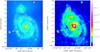 |
Fig. 1. Total intensity image of M 51 at 3 GHz with a resolution of 10″ × 7″, shown as contours, overlaid onto a Hα image (Kennicutt et al. 2003) (left) and with a resolution of 15″ in color scale in units of Jy beam−1 (right). The contours are drawn at [8, 16, 32, 64, 128, 256] × 30 μJy beam−1 (left). The beam size is shown in the top left corner. We note that this is the Stokes I image from only one spectral window that has a bandwidth of about 100 MHz (see Sect. 3.1 for explanation). |
The integrated total flux density of M 51 amounts to 703 ± 1 mJy at 3.05 GHz. Table 2 lists flux densities of M 51 observed between 151 MHz and 22.8 GHz and the corresponding references. Figure 2 shows the total integrated radio continuum spectrum of M 51 between 151 MHz and 22.8 GHz. The green diamonds in Fig. 2 show the integrated total intensity from the nine spectral window images across the S-band. The flux densities of the spectral window images are in excellent agreement with the power-law fit performed using the archival Stokes I data at multiple frequencies, where the spectral index α is defined as Iν ∝ να. This shows that our observations recover the right flux density level, and thus the data do not suffer from missing large-scale flux densities due to lack of short antenna spacings. The rms noise level in the total intensity spectral window image at 3.05 GHz amounts to about 30 μJy beam−1 at 10″ × 7″ resolution and 60 μJy beam−1 at 15″ resolution.
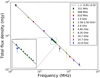 |
Fig. 2. Total integrated radio continuum spectrum of M 51 with a fitted power law, giving a total spectral index αtot = −0.81 ± 0.05. The flux densities and references are listed in Table 2. Bottom left corner: zoom in to the S-band frequency range with the integrated flux densities of the spectral window images. The data points marked with * in the legend are from this work. |
Integrated total radio continuum flux densities of M 51.
3.2. Separation of thermal and non-thermal emission
In star-forming galaxies, such as M 51, the radio continuum emission originates from a mix of synchrotron (non-thermal) and thermal free-free emission. The relative contribution of the free-free emission increases towards higher frequencies making it important to subtract its contribution from the total intensity at frequencies of our observations for the determination of the degree of polarization of synchrotron emission. To estimate the free-free emission in spatially resolved M 51, we use the mid-infrared emission as its tracer. Following Murphy et al. (2008), the free-free flux density (Sth, ν) at a frequency ν is related to the flux density at 24 μm as
 (3)
(3)
Here, Te is the electron temperature, assumed to be 104 K.
We used the Spitzer-MIPS 24 μm map of M 51, observed as a part of the SINGS (Kennicutt et al. 2003). This map is available at 6″ angular resolution in units of MJy sr−1. We first converted the 24 μm emission to Jy beam−1 units and then applied Eq. (3) to obtain the map of free-free emission at the desired frequency, in our case, at 3.05 GHz. The free-free emission map was then subtracted from the total intensity map (Fig. 1, right-hand panel) by aligning it to the same coordinate system and convolving it to 15″.
Using this method, the galaxy-integrated thermal fraction4 at 3 GHz (fth, 3 GHz) of M 51 is found to be 0.14 ± 0.01, which corresponds to fth, 1 GHz = 0.11 ± 0.07. This is consistent with Klein et al. (2018) and locally agrees with the fth, 1 GHz map of Heesen et al. (2014) within about 10% in bright star-forming regions and ≲5% in the low surface brightness inter-arms. With a relative error5 of ±a in the estimated fth, the relative error in the synchrotron emission fraction (Δ fnth, where fnth = 1 − fth) is given by Δfnth = [1 − (1 ± a) fth] / [1 − fth] (Basu et al. 2017b). This means that an error of up to 20% (a = 0.2) in a region with fth = 0.4 (0.2) yields a relative error in the estimated synchrotron emission of about 15 (5)%. This will not significantly affect the results presented in the rest of this paper.
The 24 μm emission traces mostly the ionized gas in star-forming regions. The estimate of the thermal radio emission based on the 24 μm emission can be uncertain by a factor as large as two on kpc scales (Leroy et al. 2012), especially in the inter-arm regions and in the outer disk. However, even such a large uncertainty would modify the degrees of non-thermal polarization in the S-band only within the typical measurement errors.
4. Polarization analysis
4.1. RM-Synthesis application
To obtain the maps in polarized intensity (PI), polarization angle (ψ), and RM, we applied RM-Synthesis to the polarization Stokes Q and U data (Brentjens & de Bruyn 2005), using the python-based code developed by Michael Bell6. With the usable frequency band (after flagging) we reach a resolution in Faraday depth of 522 rad m−2, a maximum detectable scale of 229 rad m−2, and a maximum detectable Faraday depth of 1357 rad m−2. RM-Clean (Heald et al. 2009), a technique to deconvolve the complex polarization from the RM Spread Function, similar to the clean algorithm used in interferometric imaging, was included in the python package and applied to the data as well. We used a step size of 2 rad m−2 in a range from −2000 to +2000 rad m−2 and cleaned down to a cut-off of 6 σQU, where σQU is the average rms noise in Stokes Q and U across the band (given in Table 1). The specifications used for RM-Synthesis and the resulting parameters are summarized in Table 3. We extracted the peak polarized intensity and the corresponding Faraday depth from the Faraday spectrum at each pixel across the galaxy to obtain the maps of polarized intensity and Faraday depth. Given the poor resolution in Faraday depth space, the Faraday spectra from different lines-of-sight show no complex nature, just a single peak, not broader than the resolution δΦ. In this case, we may assume RM ≡ Φ. Therefore, we adopt the notation “peak RM” (or just “RM”) throughout this paper. However, we note that due to the poor resolution in Faraday depth, we cannot rule out that there are several components in the Faraday spectrum hidden in the broad peak, resulting from different components along the line-of-sight contributing to the observed RM.
RM-synthesis parameters and specifications in the S-band.
To ensure that the polarization analysis is not affected by bandwidth depolarization, we examined the amount of depolarization within the observational bandwidth. The reduction of the degree of polarization by bandwidth depolarization depends on the amplitude of the observed RM, the observational frequency, and the bandwidth. The effect is strongest at low frequencies. For the S-band (with subbands of 128 MHz width in the spectral window images), a |RM| of 500 rad m−2 would reduce the degree of polarization systematically by about 5%, but the maximum observed |RM| in the S-band is a factor of about two smaller (see Sect. 4.3). Also at higher frequencies (X- and C-bands), the amplitude in |RM| does not exceed the limit that reduces the degree of polarization by more than 5%. Therefore, bandwidth depolarization does not significantly affect our analysis.
4.2. M 51’s magnetic field in the plane of the sky revealed by the S-band data
In this section, the magnetic field component perpendicular to the line-of-sight across M 51 is discussed. Information on this component is given by the spatial distribution of the polarized intensity PI and the intrinsic polarization angle ψ07 that, rotated by 90 degrees, shows the magnetic field orientation in the plane of the sky.
4.2.1. Polarized intensity and magnetic field structure
The polarized intensity in the S-band overlaid with the polarization angles rotated by 90 degrees indicating the magnetic field orientation is shown in Fig. 3. The left panel shows the polarized intensity as contours overlaid on the Hα image from Kennicutt et al. (2003) at 10″ × 7″ resolution. The right panel shows the polarized intensity at 15″ resolution as rainbow color scale. The polarized intensity at 15″ resolution is used in this paper for analysis. The polarization angles are corrected for Faraday rotation via  , where ψ0 is the intrinsic polarization angle,
  m2 is the weighted average of the observed range in λ2, and ψ is the observed polarization angle at the average wavelength of the S-band.
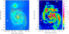 |
Fig. 3. Linearly polarized intensity image of M 51 at 3 GHz with a resolution of 10″ × 7″ overlaid onto a Hα image (Kennicutt et al. 2003) (left) and with a resolution of 15″ in color scale in units of Jy beam−1 (right). The contours in the left panel are drawn at [8, 12, 16, 24, 32] × 6 μJy beam−1. The polarized intensity maps are overlaid with the polarization E + 90°-orientations, corrected for Faraday rotation to show the magnetic field structure. Data of the polarization orientations are only shown where the signal-to-noise ratio in polarized intensity exceeds five. The beam size is shown in the top left corner. |
The magnetic field structure shows a spiral pattern. Compared to the total intensity, which shows a clear correspondence with the optical spiral arms, the spatial distribution of the polarized intensity across the galaxy is more complicated. Some parts of polarized emission coincide well with the optical spiral arms seen in Hα, but at some locations the peak of polarized emission is located in the inter-arm regions, as discussed in studies at other frequencies (e.g., Fletcher et al. 2011).
4.2.2. Field ordering
To visualize the degree of order of the magnetic field in M 51, we compute a map of the degree of polarization by dividing the polarized intensity by the non-thermal intensity map at 3.05 GHz. The fractional polarization map is shown in the left panel of Fig. 4, while the error map is shown in the right panel. The observed degree of polarization varies from a few percent in the inner spiral arms up to about 40–50% in the inter-arm regions. The low values (< 10%) in the central region and at the locations of the gas spiral arms probably originate from star-forming activity, generating small-scale fields on the turbulence scale (50–100 pc) and/or fields tangled on larger scales, but smaller than the size of the telescope beam. The extremely high values of up to 100% in the outskirts of M 51 arise from a low a signal-to-noise ratio in the non-thermal intensity map, have large errors (50–100%), and are not physical.
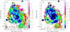 |
Fig. 4. Map of the observed degree of polarization of the non-thermal emission at 3 GHz at 15″ resolution (left) and the corresponding error map (right), overlaid with the total intensity contours at [4, 8, 16, 32] × 60 μJy beam−1. Data are only shown where the signal-to-noise ratio in polarized intensity exceeds five. The synthesized beam is shown in the top left corner. |
A closer look at the observed degree of polarization in Fig. 4 reveals a radial increase from about 2% in the center up to about 40% at the outer spiral arms in the S-band. We computed the degree of polarization as a function of the radius determined from the average non-thermal and polarized intensities at 15″ resolution in radial rings (Fig. 5). The error bars in Fig. 5 are derived from the rms noise in the maps in the non-thermal intensity, Stokes Q, and U maps.
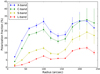 |
Fig. 5. Azimuthally averaged degree of polarization of the non-thermal emission as a function of radius in M 51, computed from our radio maps at 15″ resolution in rings of 20″ radial width in the plane of the galaxy (with inclination l = −20° and position angle PA = − 10°) out to a maximum radius of 240″ (this refers to the middle of the ring). The error bars are calculated from the rms noise in the maps from which the degrees of polarization are derived. |
The degree of polarization increases from a few percent at small radii up to about 20% at larger radii. Additionally, we show the degree of polarization as a function of radius at higher (the X- and C-bands, from Fletcher et al. 2011) and lower (the L-band, from Mao et al. 2015) frequencies. The trend of an increasing degree of polarization towards larger radii is similar at all frequencies, whereas the amplitudes are significantly different (about a factor of three larger at higher frequencies compared to the S-band and the L-band). The lower amplitudes in the S-band and the L-band arise from the fact that we see less deeply into the disk than at higher frequencies. The S-band polarization data probe the halo and a layer above the disk where the disk emission is partly depolarized. The L-band polarization data probe only the front part of the halo, while the disk emission is completely depolarized.
There are two bumps in the degree of polarization as a function of radius plot at 100″ (∼3.7 kpc) and about 200″ (∼7.4 kpc). The rings at these radii well coincide with the radius of the inter-arm regions between the two well-pronounced gas spiral arms in M 51. The inter-arm regions are believed to host well-ordered magnetic fields, which results in a high degree of polarization. If this is the case, we expect the minima to appear at the position of the gas spiral arms where the turbulent field is stronger and hence the degree of polarization is lower. Indeed, the minima in Fig. 5 occur at the galaxy center and at a radius of about 140″ (∼5.2 kpc), which is approximately the radius at which both spiral arms are located. The degree of polarization at all frequencies changes by a factor of ∼1.4 between the arm and inter-arm regions. We note that the rings do not coincide with the spiral arms due the pitch angles of the spiral arms8. Still, because the strongest emission from both prominent spiral arms and the weakest emission from inter-arm regions, appear within the same rings, this approximation is sufficient for the purpose of this study.
4.3. M 51’s magnetic field along the line-of-sight revealed by the S-band data
The RM map of M 51 in the S-band is shown in Fig. 6. It is clipped by the polarized intensity map using five times the average rms noise in Stokes Q and U, σQU. The error map is shown as well. The error in RM is calculated as
 (4)
(4)
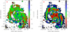 |
Fig. 6. RM map of M 51 at 15″ resolution (left) and the corresponding error map (right), calculated using Eq. (4). Data are only shown where the signal-to-noise ratio in polarized intensity exceeds five. The beam size is shown in the top left corner. |
where S/NPI is the signal-to-noise ratio in polarized intensity and δΦ is the resolution in Faraday depth (e.g., Iacobelli et al. 2013). The RM map is corrected for the Milky Way foreground via RM =RMobs − RMMW assuming a contribution of RMMW = +13 ± 1 rad m−2 (Mao et al. 2015).
The RM distribution shows a mean of about −3 rad m−2 with a standard deviation of 46 rad m−2 (Fig. 7, see also Table 4). The RM values range from about −150 rad m−2 to +150 rad m−2. This is comparable to the range of RM found between the C- and X-bands (4.85 GHz and 8.35 GHz) by Fletcher et al. (2011), but a factor of five larger than the range found in the L-band (1–2 GHz) by Mao et al. (2015) of about ±30 rad m−2 (compare Table 4). The varying ranges in RM found at different frequencies result from polarized emission probing different physical depths: the polarized signal at short wavelengths originates from the disk and experiences strong Faraday rotation on the way through the galaxy along the line-of-sight when passing through the turbulent mid-plane where large fluctuations in electron densities and magnetic fields produce a much larger RM. At longer wavelengths (around 20 cm) the signal from the disk is almost completely depolarized by wavelength-dependent Faraday depolarization effects (including differential Faraday rotation and internal and external Faraday dispersion) and the remaining signal originates in the halo, experiencing only little Faraday rotation, which is reflected in the small amplitude of RM detected in the L-band.
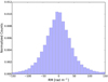 |
Fig. 7. Histogram of the RM map at 15″, shown in Fig. 6. Data were only used where the signal-to-noise ratio in polarized intensity exceeds five. The distribution has a mean of −3 rad m−2 and a standard deviation of 46 rad m−2. |
Mean RM and RM dispersion values from different frequency bands.
Also the RM dispersions (given by the standard deviation of the RM distribution in Fig. 7) have different values at different frequencies: the RM dispersion between 4.85 GHz and 8.35 GHz, hence in the disk, have the highest value (σRM, X/C − band = 50 rad m−2)9, whereas the standard deviation in the L-band, hence in the halo, is significantly smaller (σRM, L − band = 14 rad m−2).
Due to the mild inclination of M 51 of −20° and the large-scale spiral structure of the magnetic field indicated by the polarization angles seen in Fig. 3, one would expect to see a large-scale signature in the RM map if the large-scale magnetic field is regular/coherent. However, the spatial RM distribution observed in the S-band in Fig. 6 has a fluctuating nature and no obvious large-scale pattern can be recognized. Fletcher et al. (2011) found a weak large-scale RM pattern only after spatial filtering. When averaging our new S-band data in sectors of several rings, the RMs are compatible with the model by Fletcher et al. (2011) (see Appendix A).
The apparent paradox between polarization angles and RMs was already discussed in Fletcher et al. (2011) who proposed that the large-scale spiral pattern seen in the polarization angles is dominated by the components of anisotropic turbulent fields on the plane of the sky, while the line-of-sight components cancel and hence do not contribute to RM.
The model of the large-scale regular field in the disk by Fletcher et al. (2011) for the radial range of 2.4 – 4.8 kpc predicts RM amplitudes of ±18 rad m−2 and ±10 rad m−2 for the m = 0 and m = 2 modes in the disk and the inclination of −20°. The much larger RM values of ±150 rad m−2 seen in Fig. 6 indicate that strong regular magnetic fields occur on scales of a few times the beam size of ∼550 pc. This fluctuating nature of the RM could be a signature of vertical fields emerging from the disk, dominating the signal in Faraday rotation. Another explanation could be tangled regular fields that contribute to RM and to polarized emission (see Sects. 6.2 and 6.3 for discussions).
5. Application of an analytical depolarization model
In this section, we explain the general features of the analytical multi-layer depolarization model developed by Shneider et al. (2014a) and compare a representative sample of model configurations to the observations between 1 and 8 GHz (between λ30 and λ3.5 cm). Shneider et al. (2014a) compared the model predictions with three data sets at 8.35 GHz, 4.85 GHz, and 1.4 GHz (λλλ 3.5 cm, 6.2 cm, and 20 cm) from Fletcher et al. (2011), Horellou et al. (1992), Neininger et al. (1996). The new S-band data at 2–4 GHz (λλ7–15 cm) lie in a critical wavelength range between the previous data sets where the model predictions strongly differ and thus will help to better constrain the depolarization model.
5.1. A multi-layer depolarization model
Shneider et al. (2014a) developed a model of the depolarization of synchrotron radiation in a multi-layer magneto-ionic medium, applied specifically to M 51. They developed model predictions for the degree of polarization as a function of wavelength and distinguished between a two-layer system with a disk and a near-side halo, and a three-layer system with a far-side halo, a disk and a near-side halo. Details are given in Shneider et al. (2014a) and Kierdorf (2019).
The model distinguishes between scenarios of different magnetic field set-ups (in terms of regular magnetic fields, isotropic turbulent magnetic fields, and anisotropic turbulent magnetic fields), where different model configurations include either one of those or a mixture of the different magnetic field set-ups, which are considered to be present in different layers (disk and/or halo).
We model the degree of polarization in normalized form (p/p0)10 as a function of wavelength under the following assumptions:
– The thermal electron density is assumed to be spatially constant in each layer, but with different values in the disk and in the halo. The magnetic field strengths are also assumed to be spatially constant in each layer, with different values for the regular and turbulent fields (isotropic and/or anisotropic).
– The model is based on the two low (large-scale) azimuthal modes of the regular field found in M 51 by Fletcher et al. (2011) (see Appendix A) and hence it neglects higher modes (azimuthal variations on smaller scales) and vertical components of the regular field in the disk and the halo.
– The intrinsic degree of polarization at λ = 0 is assumed to be p0 = 70% everywhere in the galaxy. This corresponds to the theoretical injection spectrum for electrons accelerated in supernova remnants with αsyn = −0.5 and was observed by Fletcher et al. (2011) in the spiral arms. In the inter-arm regions, the average αsyn of −1.1 gives an intrinsic degree of polarization of p0 = 76%. Assuming p0 = 70% instead would give an overestimation of (p/p0) by about 8%.
– The anisotropy of turbulent magnetic fields is considered as the result of amplification of the components of the turbulent field, caused by compression in spiral arms and by shear from differential rotation, whereas the vertical field component remains unchanged. Anisotropic turbulent fields on scales smaller than the telescope beam contribute to polarized intensity and to depolarization (via Faraday dispersion), but not to RM.
– Several wavelength-dependent depolarization mechanisms were considered: (1) differential Faraday rotation caused by regular magnetic fields, (2) internal Faraday dispersion caused by turbulent magnetic fields (isotropic or anisotropic) within the emitting region, and (3) external Faraday dispersion caused by turbulent magnetic fields (isotropic or anisotropic) in front of the emitting region.
– In the case where turbulent magnetic fields are “switched on”, wavelength-independent depolarization (beam depolarization) is considered as well.
– The case of Faraday depolarization caused by gradients of RM across the telescope beam (Sokoloff et al. 1998) is not taken into account. This could underestimate the amount of depolarization.
– Depolarization effects from the Galactic foreground are assumed to be negligible.
The model parameters and their values used by Shneider et al. (2014a) are given in Table 5. Most parameters were fixed, while for the strengths of the regular and turbulent fields (constant along azimuthal angle in one radial ring) physically reasonable values were chosen to make the model consistent with the observations available at that time in one example region located in that ring. Surprisingly, the strengths of the regular field B in Table 5 are larger than those estimated by Fletcher et al. (2011) from the model of the large-scale field for the same radial ring, which are 1.4 ± 0.1 μG and 1.3 ± 0.3 μG for the disk and halo, respectively. Similarly large regular field strengths in disk and halo were found by fitting these two parameters to the data in 18 azimuthal sectors per radial ring for four different rings (Shneider et al. 2014b). Potential reasons of this discrepancy will be discussed in Sect. 6.3.
Model parameter values used by Shneider et al. (2014a).
In this paper, we discuss some representative depolarization model configurations from Shneider et al. (2014a), as summarized in Table 6. In Fig. 8, those model predictions for a two-layer (top panel) and three-layer (bottom panel) system are shown for region “A” (marked in Fig. 9), the same that was analyzed by Shneider et al. (2014a). We discuss model configurations with purely regular fields in disk and halo and configurations that contain regular plus turbulent magnetic fields. We note that for the three-layer model the near-side and far-side halo are assumed to have identical properties, that is, the halo is symmetric with respect to the disk.
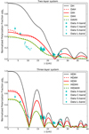 |
Fig. 8. Normalized degree of polarization as a function of wavelength for a two-layer system (top) and a three-layer system (bottom) in M 51. The plots show some representative model configurations from Shneider et al. (2014a). The observed degrees of polarization in region “A” are displayed with error bars. None of the model configurations can fit the data in the S-band (around ∼10 cm). All model profiles featured have been constructed from the set of parameters given in Table 5 (but using α = 1 for the halo): a regular field strength of 5 μG in the disk and in the halo, a disk turbulent field of 14 μG, and a halo turbulent field of 4 μG (see Table 6 for nomenclature and description of the model types listed in the legend). |
Model configurations for a two-layer system.
In the case of purely regular magnetic fields (model DH – black solid line), the intrinsic degree of polarization (at λ = 0) starts at its theoretical maximum (chosen to be 70%). The overall trend is a sinc-like function, as expected for a uniform slab (a uniform slab is a volume containing uniformly distributed thermal electrons and regular magnetic field lines, causing differential Faraday rotation). All other model configurations contain turbulent magnetic fields (DAH, DIH, DIHI, and DAIHI; see Table 6). Compared to scenarios with purely regular magnetic fields, turbulent fields significantly decrease the intrinsic degree of polarization at λ = 0 due to wavelength-independent depolarization by turbulent fields (beam depolarization). Comparing models DH and DAH, we find that the nulls appear at the same wavelengths, namely at ∼λλ 23 and 33 cm (in case of the two-layer system). The nulls appear at wavelengths depending on the RM of the layer. RM is however dependent on the regular magnetic field strength, which is assumed to be equal in the disk and halo. The turbulent field in model DAH attenuates the amplitude of the degree of polarization. Since the regular magnetic field strength is equal in the disk and the halo and therefore the RM is the same for models DH and DAH, the nulls appear at the same wavelength.
Replacing the anisotropic turbulent fields in the disk by isotropic turbulent fields (compare red solid and red dashed line in Fig. 8) only decreases the intrinsic degree of polarization at short wavelengths by a few %. The reason is that, in addition to polarized emission from regular fields, anisotropic turbulent fields contributes to the polarized signal whereas for purely isotropic turbulent fields the polarized signal vanishes.
5.2. Adapting the model to the observations between 1–8 GHz
We compared the observed degree of polarization as a function of wavelength with the model predictions in several representative regions in the galaxy, marked in Fig. 9. Before we discuss the results in all selected regions (Sect. 5.3), we explain the procedure on the basis of the original region for which Shneider et al. (2014a) compared the model with the data (region marked with “A” in Fig. 9). This region has an azimuthal angle centered at ϕ = 100° and radial boundaries of 2.4–3.6 kpc. This region was chosen because it has a high signal-to-noise ratio in polarized and non-thermal intensity. The values of the degree of polarization in all available frequency bands are given in Table C.1. We use the mean values of Stokes I and PI in the region to calculate the fractional polarization. The errors are calculated from the mean error of Stokes Q and U in the region. To get the non-thermal polarization fraction, we subtracted the thermal emission (see Sect. 3.2) in Stokes I from the total intensity by using the mean value of the thermal fraction in each considered region. Combining all data, we end up with 45 data points across 1–8 GHz (λλ3–27 cm).
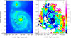 |
Fig. 9. Optical image (left) and degree of polarization at 3 GHz (right) of M 51 with the regions (marked with black boxes) in which we compared the observed degree of polarization as a function of wavelength to the depolarization model of Shneider et al. (2014a). |
The size of the region is chosen such that there are enough independent turbulent cells within the considered region to have deterministic expressions for the observed degree of polarization. The turbulence cell size d (in pc) is given as (Fletcher et al. 2011)
![Mathematical equation: $$ \begin{aligned} d \simeq \left[\frac{D\,\,\sigma _{\mathrm{RM,D}}}{0.81 \,n_{\mathrm{e}}\, b_{\parallel }\, L^{1/2}}\right]^{2/3}\,, \end{aligned} $$](/articles/aa/full_html/2020/10/aa37847-20/aa37847-20-eq8.gif) (5)
(5)
where σRM, D is the RM dispersion in the disk (assumed to be 15 rad m−2 in the model), D is the beam size (in pc), ne is the thermal electron density (in cm−3), b∥ the turbulent field strength along the line-of-sight (in μG), and L the path length through the medium (in pc). For a turbulence cell size of 55 pc, our beam of 15″ (∼550 pc) contains about 100 turbulent cells. The considered regions contain about 5 beams, hence about 500 turbulent cells. This is sufficient to be deterministic (Sokoloff et al. 1998).
By comparing the observed degrees of polarization over a larger number of frequencies to the various model predictions in Fig. 8, we can rule out model configurations with only regular magnetic fields in the disk and halo (DH) since the observed data deviate the most (a factor of four lower in the S-band). This is in agreement with observations of turbulent magnetic fields in the ISM of spiral galaxies (e.g., Beck 2016). Especially at short wavelengths model DH has a degree of polarization close to the intrinsic value without wavelength-independent depolarization (at λ = 0). If turbulent fields are present, beam depolarization is always present because the beam of our observation does not resolve the scale of turbulence, so that the intrinsic degree of polarization is about half of the theoretical maximum.
Surprisingly, none of the model predictions with the parameter values given in Table 5 are in agreement with the observed data in the S-band. For the two-layer system, the data points deviate by a factor of up to about two from the model predictions, whereas for the three-layer case, some data points are well reproduced by the model predictions, but the lines drop to zero at λ ≈ 11 cm (≈2.7 GHz) and at λ ≈ 17 cm (≈1.8 GHz), which is clearly ruled out by the observed data. In any case, our new S-band data are crucial to evaluate whether the model predictions fit the observations.
The Shneider et al. (2014a) model contains many parameters. Some of them, specifically the thermal electron densities, the path lengths L, and the turbulence cell sizes in disk and in halo (Table 5), as well as the fitted parameters of the different magnetic Fourier modes in disk and halo (pitch angle, azimuth, and amplitudes of the Fourier modes), were constrained using prior studies (Berkhuijsen et al. 1997; Fletcher et al. 2011). The most uncertain parameters are the regular and turbulent magnetic field strengths and the thermal electron densities in the disk and in the halo, for which the local values could be significantly different from the global estimates.
To understand the model and the influence of the parameters, we developed an interactive tool in Python where some selected model parameter values (such as the regular and turbulent magnetic field strengths and also the thermal electron densities in the disk and halo) can be varied to visually inspect how well the model matches the data with physically reasonable parameter values (see Fig. C.1). We vary these parameters over the whole range of physically reasonable values until we find the optimum combination. To judge the quality of this “eye-ball fit”, we calculate a reduced χ2 value (with 45 data points and five free parameters). We do not perform an automated least-square fit because the convergence of the fit highly depends on the initial parameters. Furthermore, the interactive tool makes it easy to visualize the changes in the degree of polarization as a function of wavelength when various parameters are modified.
Figure 10 shows the DAH model configuration with the optimum set of parameters for region “A” (red dashed line). The magnetic field strengths and electron densities are listed in Table 7 (columns 3 and 4) and are all physically plausible values. The uncertainties are obtained by varying the optimum value of each parameter found for the minimum reduced  (keeping the others fixed) towards smaller and larger values until the reduced χ2 becomes larger by 50% compared to
  . This criterion is the same as that used by Shneider et al. (2014b). Although our procedure cannot reveal the detailed shape of the five-dimensional surface in parameter space where χ2 increases by 50%, it measures the diameters along the five parameter axes.
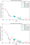 |
Fig. 10. Model DAH (red dashed line) for a two-layer system (top panel) and a three-layer system (bottom panel) in M 51 with the optimum set of parameters to represent the observed degree of polarization at multiple wavelengths in the region marked “A” in Fig. 9. The parameter values are given in Table 7. |
Our values differ significantly from those used by Shneider et al. (2014a) (Table 7, column 2): the field strengths in the disk are larger, while the electron densities are smaller. Compared to Shneider et al. (2014a), the product B ⋅ ne for the two-layer model is larger for the disk and smaller for the halo, hence Faraday depolarization by regular disk fields is more important in our study. On the other hand, Faraday depolarization by turbulent disk fields (depending on bd ⋅ ne, d) is smaller than in Shneider et al. (2014a).
Parameter values adopted by Shneider et al. (2014a) (Col. 2) and optimum sets of parameters from our study for the DAH model configuration (Cols. 3–7).
The nulls in the three-layer system (bottom panels of Figs. 8 and 10) appear at wavelengths where polarized emission from the far-side halo and the near-side halo are canceled by differential Faraday rotation. This is possible because the physical properties of the far-side and near-side halos are assumed to be identical and the polarized emission from the halo strongly dominates over that of the disk.
For the three-layer system it is not possible to remove the nulls in the model by changing any of the free parameters within its physically viable range. The same holds for the other three-layer model configurations tested in our study. This suggests that we do not detect polarized emission in the S-band and the L-band from the far-side halo because the signal emitted by the far-side halo gets almost completely depolarized by the disk, or that the dominance of the halo emission is not valid (see Sect. 6.4 for a discussion).
In their second paper, Shneider et al. (2014b) fitted two parameters, the average field strengths of the regular field in the disk and halo, to the observed degrees of polarization at λλλ3, 6, and 20 cm, averaged in 18 azimuthal sectors in each of four rings across the galaxy M 51. For each ring they assumed fixed values of the thermal electron density in disk and halo and a set of nine fixed values of the turbulent field strength. They used the magnetic field model for the four rings from their first paper (Shneider et al. 2014a) and performed a statistical comparison via χ2 analysis of predicted to observed polarization data to get the best-fit regular magnetic field strengths in the disk and halo at each ring. They found that a two-layer system provides better fits compared to the three-layer model, although the best-fit magnetic field strengths for a three-layer system are comparable.
Our new S-band data confirm that the two-layer model is preferred over the three-layer model by directly comparing the model predictions with observations by visual inspections, without performing the fitting procedure as it was done by Shneider et al. (2014b), but also allowing the electron density and turbulent field strength to vary. Including the new S-band data, our analysis gives stronger evidence for this statement because in this wavelength range the model predictions differ most.
We have also tested two-layer model configurations that include turbulent fields in the halo (compare Table 6). Basically for all considered model configurations optimum parameter sets can be found with similarly good reduced χ2 values. It is not surprising that the optimum parameter sets with an additional parameter, which means adding another degree of freedom, represent the data well since we can already find good representations for a simpler case. Hence, we exclude model configurations with turbulent fields in the halo. Although we do see signatures of random magnetic fields in the halo from the L-band data (Mao et al. 2015), their effect on the modeling procedure is likely weak.
The model configurations DAH and DIH can be represented with almost equal field strengths and electron densities. Therefore, we cannot distinguish whether the turbulent field in the disk is isotropic or anisotropic in region “A”.
5.3. Results from different regions
Using the interactive tool, we found optimum sets of parameters of the DAH model also for the observed polarization fractions in three regions located in the same radial ring of 2.4–3.6 kpc: A neighboring region with respect to the original region (marked with “A1” in Fig. 9, at azimuthal angle 140°), in a region located in the inter-arm on the western side of the galaxy (region “B”, at azimuthal angle 285°), and in a region located at a spiral arm with low signal-to-noise in polarized intensity (region “C”, at azimuthal angle 190°).
All discussed regions have low RM values in the X-, C-, to L-band (up to maximum of 25 rad m−2), hence, the contribution from a possible vertical magnetic field component is negligible.
The results are listed in Table 7, while Fig. 11 shows the DAH model configurations with the optimum parameter sets for the degrees of polarization observed in regions “A1”, “B”, and “C”. The relative uncertainties in the regular field strengths in disk and halo, Bd and Bh, in Table 7 are between 8% and 16% (except for Bd in region “C” that cannot be constrained well). With the availability of the new S-band data, the model parameters are constrained better, with relatively lower uncertainty, as compared to Shneider et al. (2014b). The relative uncertainties in the other parameters in Table 7 are of the same order (except for the thermal densities in region “C”).
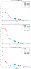 |
Fig. 11. Model DAH (red dashed line) for a two-layer system in M 51 with the optimum set of parameters to represent the observed degree of polarization at multiple wavelengths in region “A1” (top), region “B” (middle), and region “C” (bottom). |
The field strengths in region “A1” are very similar to those found in region “A”. In the inter-arm region “B” the degree of polarization is very large at high frequencies (up to 50% at 8.5 GHz or 3.5 cm), close to the theoretical maximum. The highly regular magnetic field is even a factor of about two stronger than the turbulent magnetic field. This confirms our current understanding of strong regular fields to be present in the inter-arm regions. The low observed RM of −6 rad m−2 suggests that the regular field component along the line-of-sight, which means in the vertical direction, is small in thís region. Our results for the spiral arm region “C” gives the smallest regular and the highest turbulent field strength, as expected for a region located in the spiral arm that contains only weak regular fields but a strong turbulent component. As for region “A”, the model configurations DAH and DIH can be represented with almost equal parameter values in all other regions.
For the ring of 4–3.6 kpc, Shneider et al. (2014b) found (also for a two-layer model) regular field strengths of Bd ≈ 9 μG and Bh ≈ 4 μG and turbulent field strengths of bd ≈ 11 μG and bh ≈ 5 μG. Our analysis shows that the field strengths vary significantly from one to another region (Table 7). As all four regions are located in the same radial ring, the model assumption of constant values within one radial ring is obviously not valid. We find regular field strengths of Bd = 8 − 18 μG in the disk and Bh = 3 − 5 μG in the halo, while the turbulent field bd in the disk varies between 11 μG and 24 μG.
Our values yield a range of total field strengths in the disk of Btot, d = 21 − 26 μG in the four regions (Table 7), which agrees well with the equipartition values in this radial range derived from the total synchrotron emission (see Fig. 8 of Fletcher et al. 2011). This indicates that most of the total synchrotron emission emerges from the disk, while the halo hardly contributes.
The thermal electron densities also vary considerably between the four regions of our analysis. The average value in the disk of ne, d ∼ 0.07 cm−3 is significantly smaller than the constant value assumed by Shneider et al. (2014a) and Shneider et al. (2014b) for this ring. This supports our approach to include the thermal electron densities as free parameters and allow them to vary within a ring.
6. Discussion
6.1. Decreasing turbulent field strength in M 51’s outskirts
The degree of polarization in M 51 increases towards larger radii (Sect. 4.2.2), which could be caused by a decrease of Faraday depolarization as a function of radius. To verify this, we calculate the depolarization between different bands. Figure 12 shows the depolarization (DP =pν1/pν2) between the S-band (3.05 GHz) and the X-band (8.35 GHz) and between the L-band (1.5 GHz) and the X-band. Indeed, DP increases towards larger radii (from 0.2–0.8 between the X-band and the S-band and from 0.1–0.4 between the X-band and the L-band), which shows that the depolarization effect becomes weaker at larger radii.
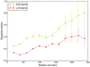 |
Fig. 12. Faraday depolarization between the S-band (2–4 GHz) and the X-band (8.35 GHz), and between the L-band (1–2 GHz) and the X-band in M 51 as a function of radius in rings of 20″ radial width. The depolarization was calculated by the ratio of the degrees of polarization at the corresponding frequencies, where DP = 1 means no depolarization and DP = 0 means total depolarization. |
Decreasing Faraday depolarization (due to decrease in Faraday dispersion) towards larger radii can be attributed to a decreasing (isotropic) turbulent magnetic field strength b, probably also accompanied by a decreasing thermal electron density (compare Eq. (8)), both of which are a consequence of decreasing star-formation rate (SFR) towards larger radii. b and SFR are closely related (e.g., Heesen et al. 2014). A decreasing turbulent field strength is evident from the total synchrotron emission that decreases towards larger radii (Fig. 1). The regular magnetic field can also contribute to Faraday depolarization (differential Faraday rotation, see Sect. 5.1) and, because its strength is expected to decrease towards larger radii, this depolarization effect is also expected to decrease.
The model fits performed by Shneider et al. (2014b) (see end of Sect. 5.2) in four rings over the radial range 2.4–7.2 kpc (65–195″) did not indicate significant radial decreases of the turbulent and regular field strengths and hence cannot explain the results shown in Fig. 12. The relative roles of the two above Faraday depolarization mechanisms should be investigated by an improved depolarization model.
At large radii, the observed degree of polarization is about 40% in the X-band (left-hand panel of Fig. 4), which is below the theoretical maximum degree of polarization of 76%11, suggesting that another depolarization mechanism is at work. The same turbulent fields responsible for depolarization by Faraday dispersion at smaller radii can also cause considerable wavelength-independent depolarization. Isotropic turbulent fields have scales smaller than the scale probed by the telescope beam and hence cannot be resolved, so that their synchrotron emission is unpolarized. If Faraday depolarization is negligible (for example, at the high frequency of the X-band), the observed degree of polarization p depends on Bord, ⊥, the strength of the ordered field in the sky plane, and b, the isotropic turbulent field (Burn 1966, corrected by Heiles et al. 1996):
 (6)
(6)
with p0 = 0.76 being the maximum degree of polarization. This allows us to determine the ratio of the isotropic turbulent field strength compared to the strength of the ordered field (regular plus anisotropic turbulent):
 (7)
(7)
Using the p values observed in the X-band (Fig. 5), the ratio b/Bord, ⊥ decreases drastically from the central region towards larger radii. (Noteworthy, in the inner parts of M 51 the X-band emission comes from disk, mostly from spiral arms. In the outer parts (at radii of about > 200″) spiral arms are faint and the disk emission is weak, so that disk and halo contribute similarly.) We get b/Bord, ⊥ ∼ 3.6 at a radius of 20″. At larger radii (> 50″), we get an average ratio between ∼1.4 in inter-arm regions (at 100″ ∼ 3.7 kpc) and in the outer disk (at 200″ ∼ 7.4 kpc), whereas ∼1.8 in regions of spiral arms at 140″ (∼5.2 kpc, compare Fig. 5).
The above field ratios cannot be directly compared with those from our two-layer depolarization model (Table 7) because Eq. (7) gives a weighted average between disk and halo. As our depolarization model did not deliver values for the turbulent field bh in the halo, we can compare b/Bord, ⊥ only with the disk values bd/Bd12, which is valid for radii of about < 200″ where the disk emission dominates. Furthermore, because  , the ratio b/Bord, ⊥ includes anisotropic fields and hence is a lower limit for the ratio b/B that was derived from the depolarization model13.
In spite of the uncertainties, good agreement of the two ratios is found for the inter-arm regions “A” and “A1” (bd/Bd ∼ 1.3), indicating that the contribution of anisotropic turbulent fields to Bord, ⊥ is small, while for the spiral arm region “C” we found bd/Bd ∼ 2.9 that is larger than b/Bord, ⊥ ∼ 1.8 for spiral arm regions, as expected for significant anisotropic turbulent fields in such regions. In the inter-arm region “B”, hosting a particularly strong regular field, bd/Bd ∼ 0.6 is significantly smaller compared to the average of ≥1.4 for inter-arm regions as estimated above. We conclude that the results applying Eq. (7) are consistent with those obtained in Sect. 5.3.
6.2. Traces of vertical fields in the disk-halo transition region of M 51
The regular magnetic field in the disk-halo transition region of M 51 is apparently dominated by fluctuations (Sect. 4.3). Table 4 gives the mean RM and RM dispersion found at the different frequency bands.
The RM dispersion expected from (isotropic) turbulent fields with turbulence size d (“cells”) can be expressed as (e.g., Beck 2016):
 (8)
(8)
which is a different version of Eq. (5). σRM increases with the square root of the number of cells N∥ along each line-of-sight because a large number of cells allows that several of them have similar field directions, so that their RMs can accumulate. On the other hand, a large number of cells N⊥ across the beam of size D averages out the RM values from individual lines-of-sight and reduces σRM. Inserting physically reasonable values of ne, b∥, L, and d into Eq. (8), we can calculate the dispersion of the RM distribution for the entire line-of-sight through M 51. We use the results from the Shneider et al. (2014a) two-layer model, that is, the mean values of the turbulent magnetic field strength of about 18 μG (divided by  to get the parallel component) and thermal electron densities of about 0.07 cm−3 in the four discussed regions, shown in Table 7. We use L = 800 pc and d = 55 pc from Table 5. With these values, we get a RM dispersion of only 12 rad m−2 in the disk. However, in Table 4, σRM is observed to be about 50 rad m−2 in the X/C-bands and in the S-band, corresponding to the disk and disk-halo transition regions, respectively. If the dispersion is caused by purely isotropic turbulent fields, we would expect to get the same σRM from Eq. (8) as those reported in Table 4.
To obtain a σRM from Eq. (8) consistent with observations (Table 4), we would need a turbulence cell size of about 150 pc in Eq. (8), assuming all other values to be correct and the dispersion caused only by isotropic turbulent fields. From observations we know that the turbulence cell size can vary, especially from the disk to the halo, but a cell size larger by a factor of three than commonly referred to the disk of M 51 (Houde et al. 2013) is hard to explain. Furthermore, in the Milky Way, different studies consistently give sizes of d between 10 pc and 100 pc (e.g., Rand & Kulkarni 1989; Ohno & Shibata 1993; Haverkorn et al. 2008), so that turbulent fields can hardly explain the large RM dispersion.
We note that a part of the dispersion of 50 rad m−2 in the observed RM distribution could arise due to the errors from measurement noise. As can be seen in Fig. 6 (right-hand panel), RM errors in the majority of the pixels are ≲15 rad m−2. We therefore believe that the discrepancy between the expected and observed σRM is real, but perhaps by only slightly less than a factor of three.
Potential sources of field disturbances are star formation-driven gas flows forming holes in neutral hydrogen (H I) with a typical size of about 1 kpc and transporting the local regular magnetic field from the disk into higher layers, causing that RMs change from one to the other edge of the hole. Heald (2012) found a co-location of a sinusoidal variation in RM and a hole observed in neutral hydrogen (H I) close to a spiral arm of the face-on nearby spiral galaxy NGC 6946. Also, Mulcahy et al. (2017) found one RM variation coinciding with a H I hole in the face-on spiral galaxy NGC 628 in the S-band. On the other hand, by comparing the position of H I hole detections in M 51 (Bagetakos et al. 2011) with our RM map at 15″ in the S-band visually, no obvious RM variation coinciding with a H I hole was found. A reason for the non-detection of RM variations coinciding with H I holes in M 51 could be the weak large-scale regular magnetic field in the disk-halo transition region and that the field is dominated by fluctuations and reversals. For such fields we do not expect to see a systematic variation in RM even if a magnetic field loop is formed and coincides with the H I hole because randomly occurring field reversals along the loop cancel out each other. Hence, a RM variation across a H I hole may only be observable in the presence of a strong large-scale regular (coherent) magnetic field component.
Promising reasons for the broadening of the observed RM distribution could be: (1) Tangled regular fields have a correlation length similar to or larger than the beam size (see Sect. 6.3 for a further discussion). (2) Vertical fields present in the disk and halo increase B∥ and RM.
Vertical fields can be generated by galactic winds, fountains, supernova remnants, or Parker instabilities (Parker 1966). Rodrigues et al. (2016) performed numerical MHD simulations of the Parker instability in a domain of size 6 kpc × 12 kpc × 3.5 kpc and computed RM maps for face-on view (their Fig. 12). RM were found to reverse on scales of 1–2 kpc. Global numerical MHD simulations of galaxies by Pakmor et al. (2018) revealed reversing signs of the wind-driven vertical field components also on scales of 1–2 kpc (see their Fig. 8). The RM maps of two synthetic galaxies were found to be similar to the RM map presented by Fletcher et al. (2011).
Observations show the presence of vertical magnetic fields in most edge-on spiral galaxies (Wiegert et al. 2015; Krause et al. 2020). Variations in field strength and direction and/or in thermal electron density lead to RM dispersion. For example, the vertical filaments in NGC 4631 change field directions on a scale of several kpc (Mora-Partiarroyo et al. 2019). Reversals on smaller scales may exist, but cannot be detected in RM maps of edge-on galaxies with the resolution of present-day observations. We conclude that a system of vertical fields with reversing directions could give rise to the large RM dispersion observed in M 51.
6.3. The complex nature of the magnetic fields in M 51
Inconsistency of RMs from regular fields. In Sect. 5.3, we report the optimum values of regular magnetic field strengths and thermal electron densities in the radial ring 2.4–3.6 kpc of M 51 derived from the observed degrees of polarization in different regions in this ring (Table 7). Field strengths and electron densities are found not to be constant along azimuthal angle in the ring, as assumed by the model, but show considerable variations. This is strengthened by comparing the RM values derived from the field strengths and electron densities in Table 7 with the observed values of RM in Fig. 6. Using the regular field strength B (in μG), the electron density ne (in cm−3) from Table 7, the pathlength L (in pc) from Table 5, and the azimuthal angle ϕ of the region, we can estimate the expected RM from Eqs. (A.2) and (A.3)14. For region “A” we expect RMd ≈ +140 rad m−2 in the disk and RMh ≈ +40 rad m−2 in the halo. For region “B”, we expect RMd ≈ −430 rad m−2 in the disk and RMh ≈ +10 rad m−2 in the halo. In the S-band we trace part of the disk (according to Fig. 12 about 40% in the considered ring) and the halo, so that a total RM of ≈ + 100 rad m−2 and ≈ − 160 rad m−2 should be observed in regions “A” and “B”, respectively. However, we measure only RM = +3 ± 20 rad m−2 and RM ∼ −6 rad m−2 in these regions (Fig. 6). For the halo, we measure RM = −3 ± 10 rad m−2 in the L-band (Mao et al. 2015) in region “A”, also much lower than expected. (The mean RM in the L-band in region “B” is not possible to determine because of low signal-to-noise.) Hence, the strengths of the regular field derived from the depolarization model are inconsistent with the observed RMs. This indicates a complex three-dimensional structure of the regular fields, as elaborated in the following.
Tangled regular fields. The time scale for a fully developed large-scale regular field generated by the mean-field (α − Ω) dynamo in a spiral galaxy is almost 10 Gyr (Arshakian et al. 2009). Interactions with M 51’s companion galaxy may distort this process and prolong the build-up time, so that the large-scale regular field may not yet have reached its saturation level. As a result, the evolving regular field could still be “spotty” and tangled, as indicated from numerical simulations (Hanasz et al. 2009; Arshakian et al. 2011; Moss et al. 2012). In terms of dynamo theory, field amplification occurs simultaneously on all scales, from the energy injection scale of turbulence to the size of the galaxy, with the smallest scales being amplified fastest (e.g., Brandenburg et al. 2012). The mean-field dynamo is always accompanied by field amplification on smaller scales, which causes tangling (see, e.g., Fig. 3 in Gent et al. 2013).
The Shneider et al. (2014a) model considers the observed degree of polarization as a function of wavelength. Faraday depolarization by a regular field (differential Faraday rotation, DFR) does not depend on the sign of the regular field. In the case of tangled regular fields that change sign along the line-of-sight, DFR in such a reversing field is the same as in the case without reversals, whereas the observed RM is smaller in the first case. Such reversals may occur on scales similar to or larger than the scale traced by the telescope beam (∼550 pc), much larger than the scale of the anisotropic turbulent field (∼55 pc). Tangled regular fields may solve the discrepancy between the values of RM obtained from multi-layer depolarization models and the observed RMs. Tangled regular fields also contribute to polarized intensity and may reduce the quest for small-scale anisotropic turbulent fields.
Tangled regular fields also contribute to RM dispersion. We propose to express the RM dispersion expected from tangled plane-parallel regular fields of strength Btang (similar to Eq. (8)) as:
 (9)
(9)
where a is the scale of field reversals (correlation scale)15. Dynamo theory predicts that regular fields with a range of scales a will be present in a galaxy (Brandenburg et al. 2012; Gent et al. 2013). Observing with higher resolution (hence, with a smaller beam size D) should yield larger values of σRM, to be tested with future observations.
6.4. Limitations of the Shneider et al. (2014a) model
In Sect. 5, we discussed the analytical multi-layer depolarization model developed by Shneider et al. (2014a), applied to the galaxy M 51. So far, this model is the only one that distinguishes between isotropic and anisotropic turbulent fields and includes multiple layers along the line-of-sight. The Shneider et al. (2014a) model has certain limitations.
We propose the refinement of the following assumptions:
– For the CRE density, Shneider et al. (2014a) assumed the same value in the disk and halo. However, this is inconsistent with the exponential scale heights of the synchrotron emission in edge-on galaxies (Heesen et al. 2018). A typical exponential scale height of hsyn ∼ 1.5 kpc gives a CRE scale height of hCR = hsyn ⋅ (3 + αsyn) /2 ∼ 3 kpc (assuming energy equipartition between CRs and magnetic fields), so that the CRE density should decrease from the disk to the halo by a factor of ∼1.4 at a height of 1 kpc above the disk plane and up to a factor of ∼5 at a height of 5 kpc. A different CRE density changes the synchrotron intensity. If the values of the CRE density in the disk and halo are different, they do not cancel out when calculating (p/p0).
– For the three-layer model it is not possible to “lift up” the zero drops of the degree of polarization as a function of wavelength by changing any of the free parameters. Even when including turbulent fields in the disk, the Sinc-function trend of the degree of polarization as a function of wavelength remains. The reason is that in the model the polarized emission from the halo always dominates the trend of the degree of polarization, because the field strength and electron density are assumed to be constant in the halo and the path length through the halo is much larger than that through the disk. These assumptions are hardly realistic and should be modified. Furthermore, model configurations including turbulent fields in the halo should be included in future analysis especially of three-layer systems, in order to suppress the Sinc-function trend caused by depolarization from the regular field.
– The depolarization model assumes the same synchrotron spectral index in disk and halo, while different values should be used according to observations in edge-on galaxies, as the result of energy losses of CREs (e.g., Schmidt et al. 2019). This is especially important at high frequencies (≳5 GHz), because the polarized emission from the relatively steeper spectrum halo could be sub-dominant compared to emission from the flatter spectrum disk. Therefore, the intrinsic degree of polarization (at λ = 0) should also be different in disk and halo.
– For calculating the turbulence cell size in M 51 via Eq. (5), Shneider et al. (2014a) used the same σRM, D = 15 rad m−2 (Fletcher et al. 2011) in the disk and halo, which is however incompatible with observations (Table 4): In the L-band (tracing only the polarized emission from the halo) we found σRM, D ≈ 14 rad m−2, while at higher frequencies σRM, D ≈ 50 rad m−2. This yields a turbulence cell size of about 90 pc in the disk and about 250 pc in the halo.
– Assuming a constant size of turbulence cells within the disk (55 pc) and within the halo (370 pc) could be too simplistic. The turbulence cell in spiral arms could be smaller compared to the size of turbulence at inter-arm locations (due to star-forming processes, which mainly takes place in the dense spiral arms, driving the turbulence). For example, for the Milky Way, Haverkorn et al. (2008) found a turbulence cell size of less than 10 pc in the gaseous spiral arms, while in the inter-arm locations the turbulence cell size amounts to about 100 pc.
The following fundamental improvements are proposed:
– Shneider et al. (2014a) only considered the degree of polarization as a function of wavelength. As discussed in Sect. 6.3, the model parameters should be checked for consistency with the observed RM values, allowing for variations of the magnetic field strengths and electron densities in disk and halo along each ring.
– Another future step would be to extend the model to fitting the observed Stokes Q(λ) and U(λ) values. This means considering not only the amplitude of the polarized signal but also the phase between Stokes Q and U and hence the polarization angles.
– The Shneider et al. (2014a) model neglects vertical components (with respect to the disk plane) of the regular magnetic field. From polarization observations of edge-on galaxies (e.g., Mora-Partiarroyo et al. 2019) we know that vertical field components exist in spiral galaxies. Some face-on galaxies show clear evidence of vertical regular fields in their RM maps, too. For example, Mao et al. (2015) found in their L-band data signature of an overall vertical magnetic field component in the halo of M 51 that produces a RM of about −9 rad m−2. From dynamo theory we know that magnetic fields in spiral galaxies has non-vanishing vertical components. For a quadrupolar magnetic field configuration, as it was considered in the discussed depolarization model, vertical field components are required to fulfill the divergence-free condition. In a quadrupolar magnetic field of M 51, the negative direction of the vertical field component (away from us) must be accompanied by an outward-directed radial field component in the disk, which is indeed observed (see Fig. 14 in Fletcher et al. 2011). Therefore, vertical field components need to be implemented in the depolarization model.
– We can test if there is a signature of a quadrupole or a dipole halo field in the equations by flipping the sign of the vertical component. This would provide an important step towards understanding the symmetry properties of different magnetic field configurations.
Still, the Shneider et al. (2014a) model already gives a good approximation for a multi-layer magneto-ionic medium and has strong advantages compared to classical depolarization models: it contains many more – galaxy specific – details and is able to decompose different layers along the line-of-sight, which is especially advantageous in case of the complicated magnetic field configuration in M 51 (having different configurations in the disk and halo).
The optimum parameter values from our interactive tool described in Sect. 5.2 can be used as initial conditions to perform an automized least-square fit or, even better, a MCMC simulation to probe the full posterior distribution of the parameter values of the depolarization model and to determine the values of the parameters accurately (if converging).
7. Summary and outlook
In this paper, we present a radio observational study of the magnetic field properties of the nearby grand-design spiral galaxy M 51. The observations were performed using the VLA providing high spatial resolution and a good image quality at a wide frequency coverage in the range 2–4 GHz (S-band) thanks to the broadband high-sensitivity receivers. Broadband polarization data allow us to probe the frequency-dependent character of the polarized emission and thus to study depolarization mechanisms caused by different underlying magnetic field configurations.
Studying M 51 in the S-band traces a so-far unknown polarized layer that is proposed to probe the transition region between the disk and halo. The goal was to make a major step towards understanding how large-scale regular magnetic fields are generated in the halo of spiral galaxies and how they are connected to the disk field. Here, we highlight some of the major findings.
We found an increasing degree of polarization in the S-band as a function of radius (Fig. 5). The Faraday depolarization calculated between different frequency bands (Fig. 12) implies a decreasing turbulent magnetic field strength and/or a decreasing thermal electron density towards larger radii in M 51.
The observed Faraday rotation measures (RMs) in the disk-halo transition region do not reveal an obvious large-scale pattern (Fig. 6), but instead show a large dispersion (Fig. 7). These results indicate that the observed RMs in the disk-halo transition region are dominated by tangled regular fields and/or vertical fields (with respect to the galaxy plane), distorting any signature of a large-scale pattern of the regular field and increasing the RM dispersion, as discussed in Sects. 6.2 and 6.3.
To get information on the field strength and structure in different layers, the new S-band polarization data were combined with VLA + Effelsberg observations in the C- and X-bands at 4.85 GHz and 8.35 GHz and with the broadband L-band (1–2 GHz) VLA data. In Sect. 5, we compared the observed degrees of polarization as a function of wavelength to a depolarization model from Shneider et al. (2014a). The new S-band data are critical to distinguish between a two-layer (disk–halo) and a three-layer (halo–disk–halo) system. A two-layer model of M 51 is preferred.
In general, we found that the model configurations need to contain regular fields in the disk and the halo, as well as turbulent fields in the disk. Anisotropic turbulent fields give a small contribution to the polarized signal and increases the intrinsic degree of polarization at short wavelengths by a few per cent compared to purely isotropic turbulent fields. The model configurations DAH and DIH (that is, regular fields in the disk and halo and anisotropic or isotropic turbulent fields in the disk) can be represented equally well with almost the same field strengths and electron densities. Therefore, we cannot distinguish whether the turbulent field in the disk is isotropic or anisotropic.
Our study provides an estimate of the regular and turbulent magnetic field strengths in nearby galaxies, independent of the widely used assumption of equipartition between the energies of magnetic field and of cosmic rays. In the three spiral arm regions we investigated, the turbulent field in the disk dominates with strengths between 18 μG and 24 μG, while the regular field strengths are between 8 μG and 16 μG. In an inter-arm region, the regular field strength of 18 μG exceeds that of the turbulent field of 11 μG (Table 7). The strengths of the regular fields in the halo are 3 − 4 μG in all four regions. (The strengths of the turbulent fields in the halo could not be determined.) The relative uncertainties of field strengths are mostly between 8% and 20%. The total field strengths in the disk are consistent with the equipartition estimates by Fletcher et al. (2011). The thermal electron density also varies considerably between the four regions of our analysis.
We found a striking discrepancy between the RMs expected from the regular field strengths from the depolarization model and the observed RMs. This indicates frequent field reversals of the regular field with correlation lengths larger than the scale traced by the telescope beam (∼550 pc), another hint to tangled regular fields (Sect. 6.3), possibly accompanied by vertical filaments of regular fields driven by outflows (Sect. 6.2). Tangled regular fields are predicted by models of evolving large-scale dynamo fields, and vertical fields are predicted by numerical simulations of Parker instabilities or galactic winds.
The depolarization model should be refined and extended (Sect. 6.4). Its systematical application to the entire galaxy, and allowing the magnetic field and electron density to vary spatially, would deliver maps of these quantities over the galaxy. Vertical fields should be included in the model because these are required to exist from dynamo theory. Significant vertical field components would leap out as outliers of the values of one or more of the parameters. This would provide knowledge on the field properties in the disk and halo of M 51 and other nearby spiral galaxies with almost face-on orientation. We also need an improved dynamo model for M 51 that includes tidal forces and a significant halo component (see Chapter 8.2 in Beck et al. 2019).
In future observations, higher angular resolution, along with higher signal-to-noise ratio in polarized intensity to reduce the error in RM, would help to investigate the detailed spatial distribution of regular fields and possible relations to dynamic phenomena in the ISM of the disk (for example, H II regions, Parker loops, supernova remnants, etc).
We showed that with broadband polarization data, depolarization mechanisms can be used as a powerful tool to probe the 3D structure of magnetic fields in galaxies. Future capabilities provided by the new Square Kilometre Array (SKA), with dramatically improved frequency coverage and excellent sensitivity for regions with weak radio surface brightness, will facilitate new studies of magnetic fields in the ISM of nearby galaxies. For this forthcoming radio astronomy era, our paper shows the path towards analyzing and interpreting broadband polarization data.
We adopt the notification “halo” for a physical layer between the synchrotron emitting disk and the observer (containing baryonic matter – not to be confused with a dark matter halo).
We used scales of 0, 6, 9, 18, 30, 45, 60, 100, and 200 arcsec.
The thermal fraction at frequency ν is defined as fth, ν = Sth, ν/Stot, ν, where Stot, ν is the total radio continuum flux density.
The relative error of fth is defined as a = ±dfth/fth, where dfth is the absolute error of fth.
Assuming a single Faraday depth component along the line-of-sight.
The pitch angle is defined as the angle between the tangent to the spiral arm and the tangent to a circle in the galaxy plane, measured at the point where the arm and the circle intersect (e.g., Carroll & Ostlie 1996).
We note that this new revised value of σRM should be used instead of the incorrect value in the Fletcher et al. (2011) paper.
We note that there is a typo in Eq. (25) of Shneider et al. (2014a): The term cos(D) in the third row needs to be replaced by cos(Ch) and in the fourth row the term cos(C) needs to be corrected to cos(Cd).
With a typical synchrotron spectral index of αsyn = −1.1 at the inter-arm regions (Fletcher et al. 2011).
Our depolarization model assumes that the regular field B is oriented parallel to the plane, so that we can assume B⊥ ≈ B for the following estimate.
We note that we considered the model setting DAH, which includes anisotropic fields. However, for the case with isotropic fields (DIH) the parameter values are almost equal in all four regions.
We also use the revised version of Eq. (6.1.4) in Kierdorf (2019), given in Eq. (B.1), to relate Bd to the mode amplitudes B0 and B2 in the disk and Bh to the mode amplitudes Bh0 and Bh1 in the halo.
The factor (a/D) applies if the beam size D is larger than a.
Acknowledgments
We thank Dr. Olaf Wucknitz for careful reading of the manuscript and the anonymous referee for valuable suggestions for improvements. We thank Drs. Carl Shneider and Anvar Shukurov for helpful discussions. A.B. acknowledges financial support by the German Federal Ministry of Education and Research (BMBF) under grant 05A17PB1 (Verbundprojekt D-MeerKAT). The VLA is operated by the National Radio Astronomy Observatory (NRAO). The NRAO is a facility of the National Science Foundation operated under cooperative agreement by Associated Universities, Inc. This work is based (in part) on observations made with the Spitzer Space Telescope, which was operated by the Jet Propulsion Laboratory, California Institute of Technology under a contract with NASA.
References
- Anderson, C. S., Gaensler, B. M., Feain, I. J., & Franzen, T. M. O. 2016, ApJ, 820, 144 [CrossRef] [Google Scholar]
- Arshakian, T. G., Beck, R., Krause, M., & Sokoloff, D. 2009, A&A, 494, 21 [NASA ADS] [CrossRef] [EDP Sciences] [Google Scholar]
- Arshakian, T. G., Stepanov, R., Beck, R., Krause, M., & Sokoloff, D. 2011, Astron. Nachr., 332, 524 [NASA ADS] [CrossRef] [Google Scholar]
- Bagetakos, I., Brinks, E., Walter, F., et al. 2011, AJ, 141, 23 [NASA ADS] [CrossRef] [Google Scholar]
- Basu, A., Mao, S. A., Kepley, A. A., et al. 2017a, MNRAS, 464, 1003 [NASA ADS] [CrossRef] [Google Scholar]
- Basu, A., Roychowdhury, S., Heesen, V., et al. 2017b, MNRAS, 471, 337 [CrossRef] [Google Scholar]
- Beck, R. 2016, A&ARv, 24, 7 [NASA ADS] [CrossRef] [Google Scholar]
- Beck, R., Chamandy, L., Elson, E., & Blackman, E. G. 2019, Galaxies, 8, 4 [CrossRef] [Google Scholar]
- Beck, R., & Wielebinski, R. 2013, Magnetic Fields in Galaxies, eds. T. D. Oswalt, & G. Gilmore, 641 [Google Scholar]
- Berkhuijsen, E. M., Horellou, C., Krause, M., et al. 1997, A&A, 318, 700 [NASA ADS] [Google Scholar]
- Berlok, T., & Pfrommer, C. 2019, MNRAS, 489, 3368 [CrossRef] [Google Scholar]
- Brandenburg, A., Sokoloff, D., & Subramanian, K. 2012, Space Sci. Rev., 169, 123 [NASA ADS] [CrossRef] [Google Scholar]
- Braun, R., Heald, G., & Beck, R. 2010, A&A, 514, A42 [NASA ADS] [CrossRef] [EDP Sciences] [Google Scholar]
- Bregman, J. N. 1980, ApJ, 236, 577 [NASA ADS] [CrossRef] [Google Scholar]
- Breitschwerdt, D., McKenzie, J. F., & Voelk, H. J. 1991, A&A, 245, 79 [NASA ADS] [Google Scholar]
- Brentjens, M. A., & de Bruyn, A. G. 2005, A&A, 441, 1217 [NASA ADS] [CrossRef] [EDP Sciences] [Google Scholar]
- Briggs, D. S. 1995, Bull. Am. Astron. Soc., 27, 1444 [Google Scholar]
- Burn, B. J. 1966, MNRAS, 133, 67 [NASA ADS] [CrossRef] [Google Scholar]
- Carroll, B. W., & Ostlie, D. A. 1996, An Introduction to Modern Astrophysics [Google Scholar]
- Ciardullo, R., Feldmeier, J. J., Jacoby, G. H., et al. 2002, ApJ, 577, 31 [NASA ADS] [CrossRef] [Google Scholar]
- Condon, J. 2015, ArXiv e-prints [arXiv:1502.05616] [Google Scholar]
- Cornwell, T. J. 2008, J. Sel. Top. Sign. Proces., 2, 793 [Google Scholar]
- Dumas, G., Schinnerer, E., Tabatabaei, F. S., et al. 2011, AJ, 141, 41 [NASA ADS] [CrossRef] [Google Scholar]
- Elstner, D., Golla, G., Rudiger, G., & Wielebinski, R. 1995, A&A, 297, 77 [Google Scholar]
- Fletcher, A., Beck, R., Shukurov, A., Berkhuijsen, E. M., & Horellou, C. 2011, MNRAS, 412, 2396 [NASA ADS] [CrossRef] [MathSciNet] [Google Scholar]
- Gent, F. A., Shukurov, A., Sarson, G. R., Fletcher, A., & Mantere, M. J. 2013, MNRAS, 430, L40 [NASA ADS] [CrossRef] [Google Scholar]
- Gioia, I. M., & Gregorini, L. 1980, A&AS, 41, 329 [NASA ADS] [Google Scholar]
- Hanasz, M., Wóltański, D., & Kowalik, K. 2009, ApJ, 706, L155 [NASA ADS] [CrossRef] [Google Scholar]
- Haverkorn, M., & Heesen, V. 2012, Space Sci. Rev., 166, 133 [NASA ADS] [CrossRef] [Google Scholar]
- Haverkorn, M., Brown, J. C., Gaensler, B. M., & McClure-Griffiths, N. M. 2008, ApJ, 680, 362 [NASA ADS] [CrossRef] [Google Scholar]
- Heald, G. H. 2012, ApJ, 754, L35 [NASA ADS] [CrossRef] [Google Scholar]
- Heald, G., Braun, R., & Edmonds, R. 2009, A&A, 503, 409 [Google Scholar]
- Heesen, V., Brinks, E., Leroy, A. K., et al. 2014, AJ, 147, 103 [NASA ADS] [CrossRef] [Google Scholar]
- Heesen, V., Krause, M., Beck, R., et al. 2018, MNRAS, 476, 158 [NASA ADS] [CrossRef] [Google Scholar]
- Heiles, C. 1996, in Polarimetry of the Interstellar Medium, eds. W. G. Roberge, & D. C. B. Whittet, ASP Conf. Ser., 97, 457 [NASA ADS] [Google Scholar]
- Högbom, J. A. 1974, A&AS, 15, 417 [Google Scholar]
- Horellou, C., Beck, R., Berkhuijsen, E. M., Krause, M., & Klein, U. 1992, A&A, 265, 417 [NASA ADS] [Google Scholar]
- Houde, M., Fletcher, A., Beck, R., et al. 2013, ApJ, 766, 49 [NASA ADS] [CrossRef] [Google Scholar]
- Hunter, J. D. 2007, Comput. Sci. Eng., 9, 90 [NASA ADS] [CrossRef] [Google Scholar]
- Iacobelli, M., Haverkorn, M., & Katgert, P. 2013, A&A, 549, A56 [NASA ADS] [CrossRef] [EDP Sciences] [Google Scholar]
- Kennicutt, R., Armus, L., Bendo, G., et al. 2003, PASP, 115, 928 [NASA ADS] [CrossRef] [Google Scholar]
- Kierdorf, M. 2019, Dissertation, University of Bonn [Google Scholar]
- Kierdorf, M., Mao, S. A., Fletcher, A., et al. 2018, Proc. IAU, 14, 319 [CrossRef] [Google Scholar]
- Klein, U., & Emerson, D. T. 1981, A&A, 94, 29 [NASA ADS] [Google Scholar]
- Klein, U., Lisenfeld, U., & Verley, S. 2018, A&A, 611, A55 [NASA ADS] [CrossRef] [EDP Sciences] [Google Scholar]
- Klein, U., Wielebinski, R., & Beck, R. 1984, A&A, 135, 213 [NASA ADS] [Google Scholar]
- Krause, M. 2019, Galaxies, 7, 54 [CrossRef] [Google Scholar]
- Krause, M., Irwin, J., Schmidt, P., et al. 2020, A&A, 639, A112 [CrossRef] [EDP Sciences] [Google Scholar]
- Leroy, A. K., Bigiel, F., de Blok, W. J. G., et al. 2012, AJ, 144, 3 [NASA ADS] [CrossRef] [Google Scholar]
- Ma, Y. K., Mao, S. A., Stil, J., et al. 2019, MNRAS, 487, 3432 [CrossRef] [Google Scholar]
- Mao, S. A., Zweibel, E., Fletcher, A., Ott, J., & Tabatabaei, F. 2015, ApJ, 800, 92 [NASA ADS] [CrossRef] [Google Scholar]
- McMullin, J. P., Waters, B., Schiebel, D., Young, W., & Golap, K. 2007, AstronomicalData Analysis Software and Systems XVI, eds. R. A. Shaw, F. Hill, & D. J. Bell, ASP Conf. Ser., 376, 127 [Google Scholar]
- Mora-Partiarroyo, S. C., Krause, M., Basu, A., et al. 2019, A&A, 632, A11 [NASA ADS] [EDP Sciences] [Google Scholar]
- Moss, D., Sokoloff, D., Beck, R., & Krause, M. 2010, A&A, 512, A61 [NASA ADS] [CrossRef] [EDP Sciences] [Google Scholar]
- Moss, D., Stepanov, R., Arshakian, T. G., et al. 2012, A&A, 537, A68 [NASA ADS] [CrossRef] [EDP Sciences] [Google Scholar]
- Mulcahy, D. D., Horneffer, A., Beck, R., et al. 2014, A&A, 568, A74 [NASA ADS] [CrossRef] [EDP Sciences] [Google Scholar]
- Mulcahy, D. D., Beck, R., & Heald, G. H. 2017, A&A, 600, A6 [NASA ADS] [CrossRef] [EDP Sciences] [Google Scholar]
- Murphy, E., Helou, G., Kenney, J., Armus, L., & Braun, R. 2008, ApJ, 678, 828 [NASA ADS] [CrossRef] [Google Scholar]
- Neininger, N., & Horellou, C. 1996, eds. W. G. Roberge, & D. C. B. Whittet, 592 [Google Scholar]
- Ohno, H., & Shibata, S. 1993, MNRAS, 262, 953 [NASA ADS] [Google Scholar]
- O’Sullivan, S. P., Brown, S., Robishaw, T., et al. 2012, MNRAS, 421, 3300 [NASA ADS] [CrossRef] [Google Scholar]
- Pakmor, R., Guillet, T., Pfrommer, C., et al. 2018, MNRAS, 481, 4410 [CrossRef] [Google Scholar]
- Parker, E. N. 1966, ApJ, 145, 811 [NASA ADS] [CrossRef] [Google Scholar]
- Perley, R. A., & Butler, B. J. 2013a, ApJS, 204, 19 [NASA ADS] [CrossRef] [Google Scholar]
- Perley, R. A., & Butler, B. J. 2013b, ApJS, 206, 16 [Google Scholar]
- Pillepich, A., Springel, V., Nelson, D., et al. 2018, MNRAS, 473, 4077 [Google Scholar]
- Rand, R. J., & Kulkarni, S. R. 1989, ApJ, 343, 760 [NASA ADS] [CrossRef] [Google Scholar]
- Rau, U., & Cornwell, T. J. 2011, A&A, 532, A71 [NASA ADS] [CrossRef] [EDP Sciences] [Google Scholar]
- Rodrigues, L. F. S., Sarson, G. R., Shukurov, A., Bushby, P. J., & Fletcher, A. 2016, ApJ, 816, 2 [NASA ADS] [CrossRef] [Google Scholar]
- Schmidt, P., Krause, M., Heesen, V., et al. 2019, A&A, 632, A12 [NASA ADS] [EDP Sciences] [Google Scholar]
- Segalovitz, A. 1977, A&A, 54, 703 [NASA ADS] [Google Scholar]
- Shapiro, P. R., & Field, G. B. 1976, ApJ, 205, 762 [NASA ADS] [CrossRef] [Google Scholar]
- Shneider, C., Haverkorn, M., Fletcher, A., & Shukurov, A. 2014a, A&A, 567, A82 [NASA ADS] [CrossRef] [EDP Sciences] [Google Scholar]
- Shneider, C., Haverkorn, M., Fletcher, A., & Shukurov, A. 2014b, A&A, 568, A83 [NASA ADS] [CrossRef] [EDP Sciences] [Google Scholar]
- Sokoloff, D., & Shukurov, A. 1990, Nature, 347, 51 [NASA ADS] [CrossRef] [Google Scholar]
- Sokoloff, D. D., Bykov, A. A., Shukurov, A., et al. 1998, MNRAS, 299, 189 [NASA ADS] [CrossRef] [Google Scholar]
- Steinwandel, U. P., Dolag, K., Lesch, H., et al. 2020, MNRAS, 494, 4393 [CrossRef] [Google Scholar]
- Stil, J. M., Krause, M., Beck, R., & Taylor, A. R. 2009, ApJ, 693, 1392 [NASA ADS] [CrossRef] [Google Scholar]
- Tully, R. B. 1974, ApJS, 27, 437 [NASA ADS] [CrossRef] [Google Scholar]
- Wang, P., & Abel, T. 2009, ApJ, 696, 96 [NASA ADS] [CrossRef] [Google Scholar]
- Wiegert, T., Irwin, J., Miskolczi, A., et al. 2015, AJ, 150, 81 [NASA ADS] [CrossRef] [Google Scholar]
Appendix A: Consistency of the new S-band data with the model of the large-scale magnetic field
To check whether we probe the transition region in the S-band, we tested if the new S-band data are compatible with the model of the large-scale regular magnetic field by Fletcher et al. (2011) who found azimuthal modes m = 0 + 2 in the disk, m = 0 + 1 in the halo in the innermost ring, and only a m = 1 mode in the halo in all other rings. To describe the disk and halo in the model, the Faraday rotation from M 51 is split into two components:
 (A.1)
(A.1)
where ϕ is the azimuthal angle in degrees, RMfg is the foreground rotation measure from the Milky Way, and ξD and ξH are parameters that allow us to model what fraction of the disk and halo are visible in polarized emission at a given wavelength. A ξ-parameter equal to 0 in the disk means that the disk is invisible in polarized emission, while the value of 1 means that we can observe the whole layer in polarization. Fletcher et al. (2011) used ξD = 0 and ξH = 1 in the L-band and ξD = 1 and ξH = 1 in the C- and X-bands.
The RMs in the disk and halo are proportional to the field components along the line-of-sight:
![Mathematical equation: $$ \begin{aligned} \begin{array}{@ll} \mathrm{RM}_{\rm D}&\propto -\left[B_r\sin (\phi ) + B_\phi \cos (\phi )\right]\sin (l) \\ \mathrm{RM}_{\rm H}&\propto -\left[B_{\mathrm{h}r}\sin (\phi ) + B_{\mathrm{h}\phi }\cos (\phi )\right]\sin (l)~, \end{array} \end{aligned} $$](/articles/aa/full_html/2020/10/aa37847-20/aa37847-20-eq29.gif) (A.2)
(A.2)
where
 (A.3)
(A.3)
are the components of the large-scale regular field in cylindrical coordinates, where (r, ϕ) are the radial and azimuthal coordinates in the galaxy plane. Equations (A.2) and (A.3) are taken from Berkhuijsen et al. (1997) (Eq. (A2)), neglecting the field component oriented perpendicular to the galaxy plane, and Shneider et al. (2014b) (Eq. (1)), respectively. B0, Bh0, B2, Bh1, and p0, ph0, p2, ph1 are the amplitudes and pitch angles of the corresponding field modes in the disk and halo, respectively. β2 and βh1 are the azimuthal angles at which the corresponding m > 0 mode has its maximum. If the field amplitudes are expressed in units of rad/m2, as in Eq. (A1) of Fletcher et al. (2011), then Eq. (A.2) above gives RMs directly.
To compare the S-band data to the model by Fletcher et al. (2011), the observed RM in the S-band was averaged in sectors of rings with 1.2 kpc width (while the resolution is 15″ = 0.55 kpc in the S-band), each with an opening angle of 20°. The error bars of RM are given by the standard deviation in each sector. The results are shown in Fig. A.1. Our data are found to be consistent with the large-scale RM variation expected from the model by Fletcher et al. (2011). However, fits with constant RM value have similar values of reduced χ2. Hence, the quality of the present S-band data does not allow to test or improve the Fletcher et al. (2011) model.
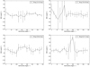 |
Fig. A.1. Rotation measure against azimuthal angle in the galaxy plane for four rings with 1.2 kpc width. The data points show the RM averaged in sectors with an opening angle of 20° with the standard deviation in each sector as the error bar. |
Appendix B: Revised version of Eq. (6.1.4) in Kierdorf (2019)
The amplitudes of the modes in disk and halo are related to the regular fields Bd and Bh in disk and halo derived by the depolarization model (Table 7) as follows:
![Mathematical equation: $$ \begin{aligned} \begin{aligned}&B_0 = B_{\mathrm{d}}\,\,\biggl [1 + \left(\frac{R_2}{R_0}\right)^2 \cos ^2(2\phi - \beta _2) \\ &\qquad \quad + 2\left(\frac{R_2}{R_0}\right)\,\cos (2 \phi - \beta _2) \cos (p_0-p_2)\biggr ]^{-1/2},\\&B_2 = B_{\mathrm{d}}\,\,\biggl [\left(\frac{R_0}{R_2}\right)^2 + \cos ^2(2\phi - \beta _2) \\ &\qquad \quad + 2\left(\frac{R_0}{R_2}\right)\,\cos (2 \phi - \beta _2) \cos (p_0-p_2)\biggr ]^{-1/2},\\&B_{\mathrm{h}0} = B_{\mathrm{h}}\,\,\biggl [1 + \left(\frac{R_{\mathrm{h}1}}{R_{\mathrm{h}0}}\right)^2 \cos ^2(\phi - \beta _{\mathrm{h}1}) \\ &\qquad \quad + 2\left(\frac{R_{\mathrm{h}1}}{R_{\mathrm{h}0}}\right)\,\cos (\phi - \beta _{\mathrm{h}1}) \cos (p_{\mathrm{h}0}-p_{\mathrm{h}1})\biggr ]^{-1/2},\\&B_{\mathrm{h}1} = B_{\mathrm{h}}\,\,\biggl [\left(\frac{R_{\mathrm{h}0}}{R_{\mathrm{h}1}}\right)^2 + \cos ^2(\phi - \beta _{\mathrm{h}1}) \\ &\qquad \quad + 2\left(\frac{R_{\mathrm{h}0}}{R_{\mathrm{h}1}}\right)\,\cos (\phi - \beta _{\mathrm{h}1}) \cos (p_{\mathrm{h}0}-p_{\mathrm{h}1})\biggr ]^{-1/2} \end{aligned} \end{aligned} $$](/articles/aa/full_html/2020/10/aa37847-20/aa37847-20-eq31.gif) (B.1)
(B.1)
Appendix C: Data and additional plots
The model configurations are the same as in Fig. 8. This tool was developed within Python 2.7 Software Foundation (Python Language Reference, version 2.716) using the module Matplotlib (Hunter 2007). The code is available on GitHub17.
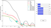 |
Fig. C.1. Interactive tool to adjust different model parameters to the data of region “A”, assuming a two-layer system. |
Observed degree of polarization in region “A” marked in Fig. 9.
All Tables
Parameter values adopted by Shneider et al. (2014a) (Col. 2) and optimum sets of parameters from our study for the DAH model configuration (Cols. 3–7).
All Figures
|
Fig. 1. Total intensity image of M 51 at 3 GHz with a resolution of 10″ × 7″, shown as contours, overlaid onto a Hα image (Kennicutt et al. 2003) (left) and with a resolution of 15″ in color scale in units of Jy beam−1 (right). The contours are drawn at [8, 16, 32, 64, 128, 256] × 30 μJy beam−1 (left). The beam size is shown in the top left corner. We note that this is the Stokes I image from only one spectral window that has a bandwidth of about 100 MHz (see Sect. 3.1 for explanation). |
| In the text | |
|
Fig. 2. Total integrated radio continuum spectrum of M 51 with a fitted power law, giving a total spectral index αtot = −0.81 ± 0.05. The flux densities and references are listed in Table 2. Bottom left corner: zoom in to the S-band frequency range with the integrated flux densities of the spectral window images. The data points marked with * in the legend are from this work. |
| In the text | |
|
Fig. 3. Linearly polarized intensity image of M 51 at 3 GHz with a resolution of 10″ × 7″ overlaid onto a Hα image (Kennicutt et al. 2003) (left) and with a resolution of 15″ in color scale in units of Jy beam−1 (right). The contours in the left panel are drawn at [8, 12, 16, 24, 32] × 6 μJy beam−1. The polarized intensity maps are overlaid with the polarization E + 90°-orientations, corrected for Faraday rotation to show the magnetic field structure. Data of the polarization orientations are only shown where the signal-to-noise ratio in polarized intensity exceeds five. The beam size is shown in the top left corner. |
| In the text | |
|
Fig. 4. Map of the observed degree of polarization of the non-thermal emission at 3 GHz at 15″ resolution (left) and the corresponding error map (right), overlaid with the total intensity contours at [4, 8, 16, 32] × 60 μJy beam−1. Data are only shown where the signal-to-noise ratio in polarized intensity exceeds five. The synthesized beam is shown in the top left corner. |
| In the text | |
|
Fig. 5. Azimuthally averaged degree of polarization of the non-thermal emission as a function of radius in M 51, computed from our radio maps at 15″ resolution in rings of 20″ radial width in the plane of the galaxy (with inclination l = −20° and position angle PA = − 10°) out to a maximum radius of 240″ (this refers to the middle of the ring). The error bars are calculated from the rms noise in the maps from which the degrees of polarization are derived. |
| In the text | |
|
Fig. 6. RM map of M 51 at 15″ resolution (left) and the corresponding error map (right), calculated using Eq. (4). Data are only shown where the signal-to-noise ratio in polarized intensity exceeds five. The beam size is shown in the top left corner. |
| In the text | |
|
Fig. 7. Histogram of the RM map at 15″, shown in Fig. 6. Data were only used where the signal-to-noise ratio in polarized intensity exceeds five. The distribution has a mean of −3 rad m−2 and a standard deviation of 46 rad m−2. |
| In the text | |
|
Fig. 8. Normalized degree of polarization as a function of wavelength for a two-layer system (top) and a three-layer system (bottom) in M 51. The plots show some representative model configurations from Shneider et al. (2014a). The observed degrees of polarization in region “A” are displayed with error bars. None of the model configurations can fit the data in the S-band (around ∼10 cm). All model profiles featured have been constructed from the set of parameters given in Table 5 (but using α = 1 for the halo): a regular field strength of 5 μG in the disk and in the halo, a disk turbulent field of 14 μG, and a halo turbulent field of 4 μG (see Table 6 for nomenclature and description of the model types listed in the legend). |
| In the text | |
|
Fig. 9. Optical image (left) and degree of polarization at 3 GHz (right) of M 51 with the regions (marked with black boxes) in which we compared the observed degree of polarization as a function of wavelength to the depolarization model of Shneider et al. (2014a). |
| In the text | |
|
Fig. 10. Model DAH (red dashed line) for a two-layer system (top panel) and a three-layer system (bottom panel) in M 51 with the optimum set of parameters to represent the observed degree of polarization at multiple wavelengths in the region marked “A” in Fig. 9. The parameter values are given in Table 7. |
| In the text | |
|
Fig. 11. Model DAH (red dashed line) for a two-layer system in M 51 with the optimum set of parameters to represent the observed degree of polarization at multiple wavelengths in region “A1” (top), region “B” (middle), and region “C” (bottom). |
| In the text | |
|
Fig. 12. Faraday depolarization between the S-band (2–4 GHz) and the X-band (8.35 GHz), and between the L-band (1–2 GHz) and the X-band in M 51 as a function of radius in rings of 20″ radial width. The depolarization was calculated by the ratio of the degrees of polarization at the corresponding frequencies, where DP = 1 means no depolarization and DP = 0 means total depolarization. |
| In the text | |
|
Fig. A.1. Rotation measure against azimuthal angle in the galaxy plane for four rings with 1.2 kpc width. The data points show the RM averaged in sectors with an opening angle of 20° with the standard deviation in each sector as the error bar. |
| In the text | |
|
Fig. C.1. Interactive tool to adjust different model parameters to the data of region “A”, assuming a two-layer system. |
| In the text | |
Current usage metrics show cumulative count of Article Views (full-text article views including HTML views, PDF and ePub downloads, according to the available data) and Abstracts Views on Vision4Press platform.
Data correspond to usage on the plateform after 2015. The current usage metrics is available 48-96 hours after online publication and is updated daily on week days.
Initial download of the metrics may take a while.