| Issue |
A&A
Volume 641, September 2020
|
|
|---|---|---|
| Article Number | A145 | |
| Number of page(s) | 5 | |
| Section | Stellar atmospheres | |
| DOI | https://doi.org/10.1051/0004-6361/202038843 | |
| Published online | 24 September 2020 | |
KELT-17: a chemically peculiar Am star and a hot-Jupiter planet★
1
Instituto de Ciencias Astronómicas, de la Tierra y del Espacio (ICATE-CONICET),
C.C 467,
5400
San Juan, Argentina
e-mail: This email address is being protected from spambots. You need JavaScript enabled to view it.
2
Universidad Nacional de San Juan (UNSJ), Facultad de Ciencias Exactas, Físicas y Naturales (FCEFN),
San Juan,
Argentina
3
Observatorio Astronómico de Córdoba (OAC),
Laprida 854,
X5000BGR,
Córdoba, Argentina
4
Instituto de Investigación Multidisciplinar en Ciencia y Tecnología, Universidad de La Serena,
Raúl Bitrán 1305,
La Serena, Chile
5
Departamento de Física y Astronomía, Universidad de La Serena,
Av. Cisternas 1200 N,
La Serena, Chile
6
Consejo Nacional de Investigaciones Científicas y Técnicas (CONICET),
Buenos Aires,
Argentina
7
Instituto de Astronomía, Universidad Nacional Autónoma de México, Ciudad Universitaria,
CDMX,
C.P. 04510, Mexico
Received:
4
July
2020
Accepted:
28
July
2020
Abstract
Context. There is very little information to be found in the literature regarding the detection of planets orbiting chemically peculiar stars.
Aims. Our aim is to determine the detailed chemical composition of the remarkable planet host star KELT-17. This object hosts a hot-Jupiter planet with 1.31 MJup detected by transits, and it is one of the more massive and rapidly rotating planet hosts seen to date. We set out to derive a complete chemical pattern for this star, in order to compare it with those of chemically peculiar stars.
Methods. We carried out a detailed abundance determination in the planet host star KELT-17 via spectral synthesis. Stellar parameters were estimated iteratively by fitting Balmer line profiles and imposing the Fe ionization balance using the SYNTHE program together with plane-parallel ATLAS12 model atmospheres. Specific opacities for an arbitrary composition and microturbulence velocity vmicro were calculated through the opacity sampling (OS) method. The abundances were determined iteratively by fitting synthetic spectra to metallic lines of 16 different chemical species using SYNTHE. The complete chemical pattern of KELT-17 was compared to the recently published average pattern of Am stars. We estimated the stellar radius using two methods: a) comparing the synthetic spectral energy distribution with the available photometric data and the Gaia parallax, and b) using a Bayesian estimation of stellar parameters using stellar isochrones.
Results. We found over-abundances of Ti, Cr, Mn, Fe, Ni, Zn, Sr, Y, Zr, and Ba, together with subsolar values of Ca and Sc. Notably, the chemical pattern agrees with those recently published for Am stars, making KELT-17 the first exoplanet host whose complete chemical pattern is unambiguously identified with this class. The stellar radius derived by two different methods agrees to each other and with those previously obtained in the literature.
Key words: stars: abundances / stars: chemically peculiar / planetary systems / stars: individual: KELT-17
Based on data obtained at Complejo Astronómico El Leoncito, operated under an agreement between the Consejo Nacional de Investigaciones Científicas y Técnicas de la República Argentina and the National Universities of La Plata, Córdoba, and San Juan.
© ESO 2020
1 Introduction
Classical A-type stars have elemental abundances that are close to solar, while Am stars present over-abundances of most heavy elements in their spectra, particularly Fe and Ni, together with under-abundances of Ca and Sc (see e.g. the recent work of Catanzaro et al. 2019, and references therein). Chemically peculiar Am stars rotate more slowly than average A-type stars (e.g., Abt 2000; Niemczura et al. 2015), and most of them belong to binary systems (e.g., North et al. 1998; Carquillat & Prieur et al. 2007; Smalley et al. 2014). These stars may host weak or ultra-weak magnetic fields driven by surface convection (e.g., Folsom et al. 2013; Blazère et al. 2016, 2020). The origin of their peculiar abundances is commonly attributed to diffusion processes due to gravitational settling and radiative levitation (Michaud 1970; Michaud et al. 1976, 1983; Vauclair et al. 1978; Alecian et al. 1996; Richer et al. 2000; Fossati et al. 2007), where the stable atmospheres of slowly-rotating A-type stars would allow the diffusion processes to operate.
The detection of planets orbiting early-type stars in general is more difficult than in late-type stars, due, for example, to the rotational broadening and lower number of spectral lines. Just in the last few years, the detection of planets orbiting A-type stars is slowly growing thanks mainly to detections using transits (e.g., Zhou et al. 2016) and direct imaging (e.g., Nielsen et al. 2019). Recently, Wagner et al. (2016) claimed the detection of a planet by direct imaging orbiting around HD 131399 A, an object classified as a possible Am star (Przybilla et al. 2017). However, this planet detection was then ruled out and attributed to a background star (Nielsen et al. 2017). Subsequent works detected planets around the likely Am star KELT-19 (Siverd et al. 2017) and the mild-Am star WASP-178 (Hellier et al. 2019). Then, the detection of planets orbiting chemically peculiar stars is particularly rare.
Recently, Zhou et al. (2016) announced the detection of a transiting hot-Jupiter planet orbiting the early-type star KELT-17. The authors reported a planet with a mass, radius, and period of 1.31 MJup, 1.52 RJup, and 3.08 days. This host star was only the fourth A-star with a confirmed transiting planet, and it is one of the most massive and rapidly rotating (~44.2 km s−1) planet hosts. The authors adopted a metallicity of −0.018 for KELT-17 (see their Table 7), that is, a solar or slightly subsolar metallicity, for this notable star.
We currently have an ongoing program aiming to study [Fe/H] in early-type stars with and without planets (Saffe et al., in prep.). The star KELT-17 is included in our sample, and a preliminary inspection of the spectra led us to suspect peculiar abundances.This was surprising, given the previously adopted solar or subsolar [Fe/H] for this star. Then, the exciting possibility of finding a planetary host with an abnormal composition motivated us to perform a detailed chemical analysis on this remarkable star, including different chemical species, to compare it with a more complete chemical pattern. This object would be the second Am star with planets detected to date, and the first one whose individual abundances are derived and compared to an Am pattern in detail.
2 Observations
The spectroscopic observations of KELT-17 were acquired at Complejo Astrónomico El Leoncito (CASLEO) between April 3 and 4, 2019. We used the Jorge Sahade 2.15 m telescope equipped with a REOSC echelle spectrograph1, selecting, as a cross disperser, a grating with 400 lines mm−1. Three spectra of the star were obtained, followed by a ThAr lamp in order to derive an appropriate wavelength versus pixel solution. The data were reduced using IRAF2 standard procedures for echelle spectra. The final spectra covered a visual range of λλ3700–6000. The resolving power R was ~13 000, and the S/N per pixel measured at ~5000 Å resulted in ~350.
Achieving a proper spectrum normalization is crucial when fitting broad spectral features like H I or strong Ca II lines in A-type stars. In echelle spectra, the normalization of orders is usually a difficult task. To obtain a reliable normalization, we proceeded as follows. First, we fit the continuum of the echelle orders without broad lines using cubic splines (6–9 pieces per order). Then, in problematic echelle orders, we toggled the wavelength scale to pixels and divided the observed spectrum by the continuum of an adjacent order (or the average of both adjacent orders if available). Finally, we normalized the resulting spectrum by a very low-order polynomial (order 1–3) to compensate for small count level differences between orders.
3 Stellar parameters and abundance analysis
The stellar parameters Teff and log g were estimated iteratively. We fit the observed Hβ and Hγ line profiles with synthetic spectra calculated with SYNTHE (Kurucz & Avrett 1981), using ATLAS12 (Kurucz 1993) model atmospheres. Starting opacities were computed for the solar values from Asplund et al. (2009). We varied temperature and gravity by adopting steps of 100 K and 0.5 dex for Teff and log g, and then we refined the grid with steps of 1 K in Teff and 0.01 dex in log g. Synthetic spectra were convolved with a rotational profile (using Kurucz’s command “rotate”) and with an instrumental profile (command “broaden”). Balmer lines of stars cooler than ~7500 K are less sensitive to gravity (e.g., Gray 2005), subsequently log g was also adjusted to satisfy the ionization equilibrium of Fe I and Fe II. Once we determined the stellar abundances, the profiles were recomputed with specific opacities for the corresponding abundances obtained. The final derived values are Teff = 7471 ± 210 K and log g = 4.20 ± 0.14 dex (see Table 1). The dispersions were adopted from differences between the adjusted values for Hβ and Hγ, and the uncertainty of the ionization equilibrium fit. These values are in good agreement with those obtained by Zhou et al. (2016), Teff = 7454 ± 49 K and log g = 4.220 ± 0.023 dex. In Fig. 1, we show a comparison of synthetic (blue dotted line) and observed spectra (black line) in the region of the Hβ line.
Projected rotational velocity v sin i was first estimated by fitting the observed line Mg II 4481.23, and then refined using the most metallic lines in the spectra. We adopted a final value of 43.0 ± 2.4 km s−1, in good agreement with the value 44.2 km s−1 derived by Zhou et al. (2016). Then, we derived abundances using spectral synthesis. There is evidence that Am stars possibly have a microturbulence velocity vmicro higher than chemically normal A-type stars (e.g., Landstreet 1998; Landstreet et al. 2009). Following this, vmicro was derived by minimizing the standard deviation in the abundance of Fe lines as a function of vmicro. We present in Fig. 2 the abundances of different Fe I lines as a function of vmicro, showing different colors for each line. In order to create this plot, vmicro was varied in steps of 0.5 km s−1. The lower panel shows the standard deviation of the different lines. This procedure was repeated while deriving Teff and log g, finally estimating vmicro = 2.50 ± 0.50 km s−1 for the star KELT-17.
The atomic line list and laboratory data used in this work are basically those described in Castelli & Hubrig (2004), updated with specialized references as described in Sect. 7 of González et al. (2014). Abundances were determined iteratively by fitting different metallic lines using the program SYNTHE. For each element, Table 2 shows the average and the total error, the number of lines, the error of the average ξ3, and the error when varying Teff, log g, and vmicro by their corresponding uncertainties eΔ. With the new abundance values, we derived both new opacities and a model atmosphere and restarted the process again. In this way, abundances are consistently derived using specific opacities calculated for an arbitrary composition using the opacity sampling (OS) method, similar to Saffe et al. (2018). Observed and synthetic spectra were compared using an χ2 function, the quadratic sum of the differences between both spectra. Synthetic abundances were varied in steps of 0.01 dex until a minimum in χ2 was reached, similarly to what was done by Saffe & Levato (2014). Abundance dispersions were estimated by quadratically adding the error of the average ξ and the abundance difference when varying Teff, log g, and vmicro by their respective errors eΔ.
Stellar parameters derived in this work for the star KELT-17.
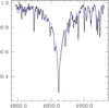 |
Fig. 1 Comparison of synthetic (blue dotted line) and observed (black continuous) spectra in the region of the Hβ line for the star KELT-17. |
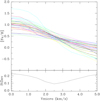 |
Fig. 2 Abundances of different Fe I lines as a function of vmicro, showing different colors for each line. Lower panel: standard deviation of the different lines. |
Abundances derived in this work for the star KELT-17.
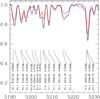 |
Fig. 3 Observed (black line) and synthetic (red and blue) spectra for the star KELT-17 between 5190 and 5230 Å. Red and blue correspond to solar and derived abundances. |
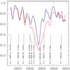 |
Fig. 4 Observed and synthetic spectra of KELT-17 in a region near the line Ca II 3933.68 Å. The colors used are the same as in Fig. 3. |
4 Discussion
In Fig. 3, we present an example of observed and synthetic spectra of the star KELT-17, for a region between 5190 and 5230 Å. The observed spectrum is shown in black, while synthetic spectra are plotted using red (solar composition) and blue dotted lines (adopted composition). We include the identification of the lines, together with their intensities (between 0 and 1). It is clear fromthis plot that KELT-17 does not match solar abundances: most metallic lines, such as Fe II and Cr II, are more intense in KELT-17. This is also evident in lines such as Y II 5200.41 Å, which is clearly present in KELT-17 and very weak adopting solar values.
In addition to over-abundances, the chemical pattern of Am stars is also characterized by subsolar values of Ca and Sc (see e.g., Catanzaro et al. 2019). We present in Figs. 4 and 5 the observed and synthetic spectra of KELT-17 near the lines Ca II 3933.68 Å and Sc II 4246.82 Å, using the same notation. Notably, the Ca II line in KELT-17 (black line) is much weaker than in a solar composition spectrum (red line). Similarly, in Fig. 5 we can see that the lines of Fe II and Cr II are more intense in KELT-17, while the line Sc II 4246.82 Å is weaker than a supposed solar-like composition. A clearer example of the weakness of Sc II in the star KELT-17 can be seen in Fig. 6. In this case, we plotted a region near the line Sc II 5526.82 Å. A solar-like composition should clearly present this line (red line), while in the spectrum of KELT-17, this line is almost absent (black line).
Over-abundances and subsolar values of species shown in Figs. 3–6 are similar to those of Am stars. A more quantitative comparison can be performed by directly comparing the abundance pattern of KELT-17 with those of Am stars in general. In Fig. 7, we show the chemical pattern as the abundance versus atomic number for the different chemical species. For the abundance pattern of Am stars (blue in Fig. 7), we used the average values recently derived by Catanzaro et al. (2019) from a sample of 62 Am stars, where vertical bars correspond to their maximum and minimum values. The abundance values derived for the star KELT-17 are shown in black. These values correspond to 16 different species identified in the spectrum: Mg I, Mg II, Si II, Ca II, Sc II, Ti II, Cr II, Mn I, Fe I, Fe II, Ni II, Zn I, Sr II, Y II, Zr II and Ba II. From this plot, we see that KELT-17 agrees in general with the chemical characteristics of Am stars.
In Fig. 8, we present the spectral energy distribution computed with ATLAS12 model atmospheres and the available photometry in different bands, adopting a Gaia parallax of 4.387 ± 0.048 mas (Gaia Collaboration 2018). We used the BT and VT Tycho-2 magnitudes (Hog et al. 2000), G, GBP and GRP Gaia DR2 magnitudes (Gaia Collaboration 2018), The Amateur Sky Survey V band (TASS, Droege et al. 2006), the Carlsberg Meridian Telescope survey r′ band (Evans et al. 2002), 2MASS J, H and Ks bands (Cutri et al. 2003), and WISE magnitudes (Cutri et al. 2012). The reddening was calculated according to the distance and position using the extinction maps of Schlegel et al. (1998)4, following the procedure of Bilir et al. (2008). From this plot, we estimated a stellar radius of 1.697 ± 0.063 R⊙. We also derived the radius through a Bayesian analysis using the PARSEC stellar isochrones (Bressan et al. 2012), from the Teff, an apparent magnitude of V = 9.23 ± 0.02 from the Tycho-2 catalog (Hog et al. 2000), and the Gaia parallax. In this way, we obtained R = 1.680 ± 0.092 R⊙ for the star KELT-17. We adopted a global solar composition when using isochrones with this chemically peculiar star, similar to previous works (e.g., Pöhnl et al. 1998; Kochukhov & Bagnulo 2006). Both estimations of the stellar radius agree with the previous determination of Zhou et al. (2016), who derived R = 1.645 R⊙. Then, the planetary radius previously estimated using the transit depth does not change significantly.
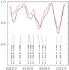 |
Fig. 5 Observed and synthetic spectra of KELT-17 in a region near the line Sc II 4246.82 Å. The colors used are the same as in Fig. 3. |
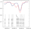 |
Fig. 6 Observed and synthetic spectra of KELT-17 in a region near the line Sc II 5526.82 Å. The colors used are the same as in Fig. 3. |
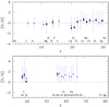 |
Fig. 7 Chemical pattern of KELT-17 (black) and average pattern of Am stars (blue). Upper and lower panels: z < 32 and z > 32. |
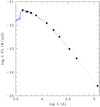 |
Fig. 8 Spectral energy distribution computed with ATLAS12 model atmospheres (blue line) and available photometry in different bands (black circles). |
5 Summary
We performed a chemical analysis of the exoplanet host star KELT-17 and found over-abundances of Ti, Cr, Mn, Fe, Ni, Zn, Sr, Y, Zr, and Ba, together with subsolar values of Ca and Sc. The chemical pattern agrees with those recently published concerning Am stars, with KELT-17 being the first exoplanet host whose complete chemical pattern is unambiguously identified with this class. We also derived the stellar radius using two different methods: obtaining good agreement between them and with those previously derived in the literature. Therefore, the classification of KELT-17 as an Am star has no significant impact on the corresponding planet parameters.
Acknowledgements
We thank the anonymous referee for suggestions that greatly improved the paper. The authors thank Dr. R. Kurucz for making their codes available to us. C.S., M.F., and J.F.G. acknowledge financial support from the CONICET of Argentina through grant PIP 0331. M.J.A. acknowledges the financial support of DIDULS/ULS, through the project PI192135.
References
- Abt, H. 2000, ApJ, 544, 933 [NASA ADS] [CrossRef] [Google Scholar]
- Alecian, G. 1996, A&A, 310, 872 [NASA ADS] [Google Scholar]
- Asplund, M., Grevesse, N., Sauval, A., Scott, P 2009, ARA&A, 47, 481 [NASA ADS] [CrossRef] [Google Scholar]
- Bilir, S., Soydugan, E., Soydugan, F., Yaz, E., et al. 2008, Astron. Nachr., 329, 835 [NASA ADS] [CrossRef] [Google Scholar]
- Blazère, A., Petit, P., Lignières, F., Aurière, M., et al. 2016, A&A, 586, A97 [NASA ADS] [CrossRef] [EDP Sciences] [Google Scholar]
- Blazère, A., Petit, P., Neiner, C., Folsom, C., et al. 2020, MNRAS, 492, 5794 [CrossRef] [Google Scholar]
- Bressan, A., Marigo, P., Girardi, L., et al. 2012, MNRAS, 427, 127 [NASA ADS] [CrossRef] [Google Scholar]
- Carquillat, J.-M., & Prieur, J.-L. 2007, MNRAS, 380, 1064 [NASA ADS] [CrossRef] [Google Scholar]
- Catanzaro, G., Busa, I., Gangi, M., Giarruso, M., et al. 2019, MNRAS, 484, 2530 [CrossRef] [Google Scholar]
- Castelli, F., & Hubrig, S. 2004, A&A, 425, 263 [NASA ADS] [CrossRef] [EDP Sciences] [Google Scholar]
- Cutri, R. M., Skrutskie, M. F., van Dyk, S., et al. 2003, VizieR On-line Data Catalog: II/246 [Google Scholar]
- Cutri, R. M., Wright, E. L., Conrow, T., et al. 2012, VizieR On-line Data Catalog: II/311 [Google Scholar]
- Droege, T. F., Richmond, M. W., Sallman, M. P., & Creager, R. P. 2006, PASP, 118, 1666 [NASA ADS] [CrossRef] [Google Scholar]
- Evans, D. W., Irwin, M. J., & Helmer, L. 2002, A&A, 395, 347 [NASA ADS] [CrossRef] [EDP Sciences] [Google Scholar]
- Folsom, C., Wade, G., & Johnson, N. 2013, MNRAS, 433, 3336 [NASA ADS] [CrossRef] [Google Scholar]
- Fossati, L., Bagnulo, S., Monier, R., et al. 2007, A&A, 476, 911 [NASA ADS] [CrossRef] [EDP Sciences] [Google Scholar]
- Gaia Collaboration (Brown, A., et al.) 2018, A&A, 616, A1 [NASA ADS] [CrossRef] [EDP Sciences] [Google Scholar]
- González, J. F., Saffe, C., Castelli, F., et al. 2014, A&A, 561, A63 [NASA ADS] [CrossRef] [EDP Sciences] [Google Scholar]
- Gray, D. F., The Observation and analysis of stellar photospheres (Cambridge: Cambridge University Press) [Google Scholar]
- Gray, R. O., Riggs, Q., Koen, C., et al. 2017, AJ, 154, 31 [CrossRef] [Google Scholar]
- Hellier, C., Anderson, D., Barkaoui, K., et al. 2019, MNRAS, 490, 1479 [CrossRef] [Google Scholar]
- Hog, E., Fabricius, C., Makarov, V., et al. 2000, A&A, 355, 27 [Google Scholar]
- Kochukhov, O., & Bagnulo, S. 2006, A&A, 450, 763 [NASA ADS] [CrossRef] [EDP Sciences] [Google Scholar]
- Kurucz, R. L. 1993, ATLAS9 Stellar Atmosphere Programs and 2 km/s grid, Kurucz CD-ROM 13 (Cambridge, MA: Smithsonian Astrophysical Obs.) [Google Scholar]
- Kurucz, R. L., & Avrett, E. H. 1981, SAO Special Report No. 391 [Google Scholar]
- Landstreet, J. D. 1998, A&A, 338, 1041 [NASA ADS] [Google Scholar]
- Landstreet, J. D., Kupka, F., Ford, H., et al. 2009, A&A, 503, 973 [NASA ADS] [CrossRef] [EDP Sciences] [Google Scholar]
- Michaud, G. 1970, ApJ, 160, 641 [Google Scholar]
- Michaud, G., Charland, Y., Vauclair, S., & Vauclair, G. 1976, ApJ, 210, 447 [Google Scholar]
- Michaud, G., Tarasick D., Charland Y., & Pelletier, C. 1983, ApJ, 269, 239 [NASA ADS] [CrossRef] [Google Scholar]
- Murphy, S. J., & Paunzen, E. 2017, MNRAS, 466, 546 [NASA ADS] [CrossRef] [Google Scholar]
- Nielsen, E., de Rosa, R., Rameau, J., et al. 2017, AJ, 154, 218 [Google Scholar]
- Nielsen, E., de Rosa, R., Macintosh, M., et al. 2019, AJ, 158, 13 [NASA ADS] [CrossRef] [Google Scholar]
- Niemczura, E., Murphy, S. J., Smalley, B., et al. 2015, MNRAS, 450, 2764 [NASA ADS] [CrossRef] [Google Scholar]
- North, P., Carquillat, J.-M., Ginestet, N., et al. 1998, A&ASS, 130, 223 [CrossRef] [Google Scholar]
- Pöhnl, H., Paunzen, E., & Maitzen, H. 2004, A&A, 441, 1111 [Google Scholar]
- Przybilla, N., Aschenbrenner, P., & Buder, S. 2017, A&A, 604, L9 [CrossRef] [EDP Sciences] [Google Scholar]
- Richer, J., Michaud, G., & Turcotte, S. 2000, ApJ, 529, 338 [NASA ADS] [CrossRef] [Google Scholar]
- Saffe, C., & Levato, H. 2014, A&A, 562, A128 [NASA ADS] [CrossRef] [EDP Sciences] [Google Scholar]
- Saffe, C., Flores, M., Miquelarena, P., et al. 2018, A&A, 620, A54 [NASA ADS] [CrossRef] [EDP Sciences] [Google Scholar]
- Schlegel, D., Finkbeiner, D. P., & Davis, M. 1998, ApJ, 500, 525 [NASA ADS] [CrossRef] [Google Scholar]
- Siverd, R., Collins, K., Zhou, G., et al. 2017, AJ, 155, 35 [NASA ADS] [CrossRef] [Google Scholar]
- Smalley, B., Southworth, J., Pintado, O., et al. 2014, A&A, 564, A69 [NASA ADS] [CrossRef] [EDP Sciences] [Google Scholar]
- Smalley, B., Antoci, V., Holdsworth, D., et al. 2017, MNRAS, 465, 2662 [CrossRef] [Google Scholar]
- Vauclair, G., Vauclair, S., & Michaud, G. 1978, ApJ, 223, 920 [NASA ADS] [CrossRef] [Google Scholar]
- Wagner, K., Apai, D., Kasper, M., et al. 2016, Science, 353, 673 [NASA ADS] [CrossRef] [Google Scholar]
- Zhou, G., Rodriguez, J., Collins, K., et al. 2016, AJ, 152, 136 [NASA ADS] [CrossRef] [Google Scholar]
On loan from the Institute d’Astrophysique de Liege, Belgium.
IRAF is distributed by the National Optical Astronomical Observatories, which is operated by the Association of Universities for Research in Astronomy, Inc., under a cooperative agreement with the National Science Foundation.
For species with one line, we adopted the average error of other elements.
All Tables
All Figures
|
Fig. 1 Comparison of synthetic (blue dotted line) and observed (black continuous) spectra in the region of the Hβ line for the star KELT-17. |
| In the text | |
|
Fig. 2 Abundances of different Fe I lines as a function of vmicro, showing different colors for each line. Lower panel: standard deviation of the different lines. |
| In the text | |
|
Fig. 3 Observed (black line) and synthetic (red and blue) spectra for the star KELT-17 between 5190 and 5230 Å. Red and blue correspond to solar and derived abundances. |
| In the text | |
|
Fig. 4 Observed and synthetic spectra of KELT-17 in a region near the line Ca II 3933.68 Å. The colors used are the same as in Fig. 3. |
| In the text | |
|
Fig. 5 Observed and synthetic spectra of KELT-17 in a region near the line Sc II 4246.82 Å. The colors used are the same as in Fig. 3. |
| In the text | |
|
Fig. 6 Observed and synthetic spectra of KELT-17 in a region near the line Sc II 5526.82 Å. The colors used are the same as in Fig. 3. |
| In the text | |
|
Fig. 7 Chemical pattern of KELT-17 (black) and average pattern of Am stars (blue). Upper and lower panels: z < 32 and z > 32. |
| In the text | |
|
Fig. 8 Spectral energy distribution computed with ATLAS12 model atmospheres (blue line) and available photometry in different bands (black circles). |
| In the text | |
Current usage metrics show cumulative count of Article Views (full-text article views including HTML views, PDF and ePub downloads, according to the available data) and Abstracts Views on Vision4Press platform.
Data correspond to usage on the plateform after 2015. The current usage metrics is available 48-96 hours after online publication and is updated daily on week days.
Initial download of the metrics may take a while.