| Issue |
A&A
Volume 641, September 2020
|
|
|---|---|---|
| Article Number | A157 | |
| Number of page(s) | 8 | |
| Section | Catalogs and data | |
| DOI | https://doi.org/10.1051/0004-6361/202038436 | |
| Published online | 24 September 2020 | |
Doppler beaming factors for white dwarfs, main sequence stars, and giant stars
Limb-darkening coefficients for 3D (DA and DB) white dwarf models⋆
1
Instituto de Astrofísica de Andalucía, CSIC, Apartado 3004, 18080 Granada, Spain
e-mail: This email address is being protected from spambots. You need JavaScript enabled to view it.
2
Dept. Física Teórica y del Cosmos, Universidad de Granada, Campus de Fuentenueva s/n, 10871 Granada, Spain
3
Department of Physics, University of Warwick, Coventry CV4 7AL, UK
4
Division of Physics, Mathematics and Astronomy, California Institute of Technology, Pasadena, CA 91125, USA
5
Department of Physics and Astronomy, University of Sheffield, Sheffield S3 7RH, UK
Received:
18
May
2020
Accepted:
27
July
2020
Abstract
Context. Systematic theoretical calculations of Doppler beaming factors are scarce in the literature, particularly in the case of white dwarfs. Additionally, there are no specific calculations for the limb-darkening coefficients of 3D white dwarf models.
Aims. The objective of this research is to provide the astronomical community with Doppler beaming calculations for a wide range of effective temperatures, local gravities, and hydrogen/metal content for white dwarfs as well as stars on both the main sequence and the giant branch. In addition, we present the theoretical calculations of the limb-darkening coefficients for 3D white dwarf models for the first time.
Methods. We computed Doppler beaming factors for DA, DB, and DBA white dwarf models, as well as for main sequence and giant stars covering the transmission curves of the Sloan, UBVRI, HiPERCAM, Kepler, TESS, and Gaia photometric systems. The calculations of the limb-darkening coefficients for 3D models were carried out using the least-squares method for these photometric systems.
Results. The input physics of the white dwarf models for which we have computed the Doppler beaming factors are: chemical compositions log [H/He] = −10.0 (DB), −2.0 (DBA), and He/H = 0 (DA), with log g varying between 5.0 and 9.5 and effective temperatures in the range 3750–100 000 K. The beaming factors were also calculated assuming non-local thermodynamic equilibrium for the case of DA white dwarfs with Teff > 40 000 K. For the mixing-length parameters, we adopted ML2/α = 0.8 (DA case) and 1.25 (DB and DBA). The Doppler beaming factors for main sequence and giant stars were computed using the ATLAS9 version, characterized by metallicities ranging from [−2.5, 0.2] solar abundances, with log g varying between 0 and 5.0 and effective temperatures between 3500 and 50 000 K. The adopted microturbulent velocity for these models was 2.0 km s−1. The limb-darkening coefficients were computed for three-dimensional DA and DB white dwarf models calculated with the CO5BOLD radiation-hydrodynamics code. The parameter range covered by the three-dimensional DA models spans log g values between 7.0 and 9.0 and Teff between 6000 and 15 000 K, while He/H = 0. The three-dimensional DB models cover a similar parameter range of log g between 7.5 and 9.0 and Teff between 12 000 and 34 000 K, while logH/He = −10.0. We adopted six laws for the computation of the limb-darkening coefficients: linear, quadratic, square root, logarithmic, power-2, and a general one with four coefficients.
Conclusions. The beaming factor calculations, which use realistic models of stellar atmospheres, show that the black body approximation is not accurate, particularly for the filters u, u′, U, g, g′, and B. The black body approach is only valid for high effective temperatures and/or long effective wavelengths. Therefore, for more accurate analyses of light curves, we recommend the use of the beaming factors presented in this paper. Concerning limb-darkening, the distribution of specific intensities for 3D models indicates that, in general, these models are less bright toward the limb than their 1D counterparts, which implies steeper profiles. To describe these intensities better, we recommend the use of the four-term law (also for 1D models) given the level of precision that is being achieved with Earth-based instruments and space missions such as Kepler and TESS (and PLATO in the future).
Key words: white dwarfs / binaries: eclipsing / stars: atmospheres
34 Tables listed in Tables A.1 and A.2 are only available at the CDS via anonymous ftp to cdsarc.u-strasbg.fr (130.79.128.5) or via http://cdsarc.u-strasbg.fr/viz-bin/cat/J/A+A/641/A157
© ESO 2020
1. Introduction
Some time ago, Loeb & Gaudi (2003) indicated the possibility of detecting exoplanets by using the Doppler beaming technique, which causes an asymmetry in the ellipsoidal modulation in the light curves of binary systems. This technique has an additional advantage because, unlike the transit method, it can be applied to practically any orbital inclination of the system.
The contribution of beaming is essential to synthesizing the light curves of a given system under study. However, such calculations are sparse in the literature. Bloemen (2015) has made an important effort in this regard, but his calculations are limited to a few systems. One of the main objectives of this short paper is to provide users with the calculations of the Doppler beaming factors for white dwarfs, stars on the main sequence, and stars on the giant branch. Such calculations cover a wide range of effective temperatures, log g, and hydrogen/metal content, and they are available for some of the most commonly used photometric systems: Sloan, UBVRI, Kepler, TESS, Gaia, and HiPERCAM.
On the other hand, some studies have shown that 3D atmosphere models compare better with observations of the center to limb variation for the Sun (see Pereira et al. 2013). Pereira et al. (2013) find a very good agreement between the limb-darkening from 3D models and observations at ultraviolet and visible wavelengths. The observations used in their paper were those of Pierce & Slaughter (1977) and Neckel & Labs (1994). However, Pereira et al. (2013) also find a poorer agreement for longer wavelengths (between 12 000 and 24 000 Å). In order to test the validity of stellar atmosphere models in other kind of stars, we present a series of computations of limb-darkening coefficients (LDCs) for white dwarfs of spectral types DA and DB, based on 3D model atmospheres and covering the same range of photometric systems as mentioned above.
We organize the paper as follows: Section 2 is dedicated to the computation of the Doppler beaming factors while Sect. 3 is devoted to the LDCs of DA-3D and DB-3D white dwarf models. Finally, in Appendix A we give brief explanations of Tables A.1 and A.2 and the data they contain. Additional material or calculations for specific photometric systems can be carried out upon request.
2. Doppler beaming factors for DA, DB, and DBA white dwarfs, main sequence stars, and giant stars
Doppler beaming is caused by the radial velocity of the stars in a double system, which displace the spectrum and modulate the photon emission rate toward the observer. The first theoretical investigation into this effect was carried out by Hills & Dale (1974) in the case of rotating white dwarfs and by Shakura & Postnov (1987) for the orbital movement of double systems.
From the observational point of view, there have also been important advances related to beaming effects. We can mention, for example: Mazeh & Faigler (2010), who detected an ellipsoidal modulation and relativistic beaming effect in the exo-planetary system CoRot-3; and Ehrenreich et al. (2011), who, using spectroscopic techniques, confirmed the relativistic beaming effect in the KOI-74 system consisting of a hot compact object around an early-type star. More recently, Wong et al. (2020) performed a consistent analysis of the KOI-964 system, which consists of a hot white dwarf and an A-type host star. With respect to the Doppler beaming factor, Wong et al. (2020) find a good agreement between theory and observational data.
In a previous paper on gravity and LDCs (Claret et al. 2020), we computed the beaming factors for four white dwarf models – DA, DB, DBA, and non-local thermodynamic equilibrium (NLTE) DA – adopting the black body approach. However, such a simple method neglects the effects of the Balmer jump, of the absorption lines, and even of the shape of the spectra, which is different from black body radiation. Furthermore, such an approach does not predict any dependence on log g or atmospheric composition. As we will see below, the local gravity and the hydrogen content (or metallicity in the case of stars) may influence the calculation of the beaming factors.
As mentioned in the Introduction, there are no systematic calculations for beaming factors that consider realistic atmosphere models of white dwarfs or stars on the main sequence or the giant branch. In the present paper, we adopt white dwarf atmosphere models of the types DA, DB, DBA, and DA-NLTE as well as the ATLAS9 models (main sequence, subgiants, and giants) for the calculation of the beaming factors for several passbands. The description of the adopted white dwarf models (DA, DB, DBA, and DA-NLTE) can be found in Claret et al. (2020, Sect. 2). The models for stars on the main sequence, subgiants, and giants used here were calculated with the ATLAS9 version. The computation of beaming factors are presented for metallicities ranging from [−2.5, 0.2] solar abundances, with log g varying between 0 and 5.0 and effective temperatures between 3500 K and 50 000 K. The adopted microturbulent velocity is 2.0 km s−1. For more detailed information on ATLAS9 features, see, for example, Castelli et al. (1997).
If we assume that the monochromatic flux is proportional to a frequency power, that is to say F(ν)∝να (Shakura & Postnov 1987), for the flux variation due to the Doppler shift (Loeb & Gaudi 2003) we have
 (1)
(1)
where vr is the radial velocity (nonrelativistic approach), c is the velocity of light in vacuum, F(ν)obs is the observed flux, and F(ν)0 is the monochromatic flux in the absence of the source motion. Eq. (1) can also be written as
 (2)
(2)
where λ is the wavelength and B(λ) is the monochromatic beaming factor,
 (3)
(3)
To compute the photon weighted bandpass-integrated beaming factors, we used the following equation:
 (4)
(4)
where S(λ) is the response function for each passband. In order to generate the average beaming factors, we adopted in Eq. (4) the transmission curves for the Sloan (u′g′r′i′z′y′), UBVRI, HiPERCAM, Kepler, TESS, and Gaia passbands. We did not consider reddening in the present calculations. We note that Eq. (4) is suitable for photon-counting devices, such as CCDs.
Figure 1 shows the comparison between beaming factors computed using Eq. (4) (continuous line) and computed adopting the black body approach (stars) for HiPERCAM and using DA models at log g = 5.0. The differences between the two recipes are notable, particularly for shorter effective wavelengths. Also noteworthy is the peak of beaming in the near-ultraviolet region around Teff = 10 000 K. This feature is also detected for less compact star models generated with the ATLAS9 code (see Fig. 2). Such behavior is related to the strength of the Balmer jump, whose effect is more intense for models with Teff ≈ 10 000 K. On the other hand, if we assume that the flux is given by the Planck function, then for large values of λ and/or Teff the calculations based on the black body approximation are closer to the predictions given by Eq. (4) using realistic atmosphere models (≈1.0), as expected.
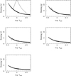 |
Fig. 1. Comparison between the beaming factors according to Eq. (4) (HiPERCAM passbands). The DA white dwarf models are represented by continuous lines and black body approximation by stars. All models are at log g = 5.0. |
Unlike the black body approach, the calculations that adopt more realistic models of stellar atmospheres predict a dependence of the beaming factors on the local gravity, as can be seen in Fig. 3. The differences in beaming factors due to log g are more prominent for shorter wavelengths, although for the y′ passband there is also a notable difference for cooler models. For hot models and long effective wavelengths, the beaming factors are almost independent of log g because the models are close to the Rayleigh-Jeans law of a black body. The effects of local gravity on the beaming factors are very interesting, particularly for the Sloan (u′) filter. In general, the strength of the Balmer jump decreases with increasing local gravity of the white dwarf model (because of nonideal gas effects), and this impacts the beaming calculations for shorter effective wavelengths. The computation of the beaming factors depends on the strength of the Balmer jump, which in turn depends on the local gravity and effective temperature. We note that the Rayleigh-Jeans law and continuum opacities also contribute to the Balmer jump.
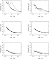 |
Fig. 3. Comparison between the beaming factors (Sloan passbands, DA white dwarf models) according to Eq. (4). Continuous lines indicate models with log g = 5.0 while stars denote those with log g = 9.0. |
In Fig. 4, we show the influence of the hydrogen abundance in the beaming factor profiles. The differences are small for longer effective wavelengths but they can be detected observationally, particularly for effective temperatures below 20 000 K and for shorter effective wavelengths. As we anticipated at the beginning of this section, realistic atmosphere models for white dwarfs are able to predict a beaming factor dependence on the local gravity and with the hydrogen content, particularly for shorter effective wavelengths.
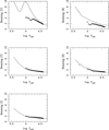 |
Fig. 4. Beaming factors for the UBVRI passbands according to Eq. (4) for log g = 5.0. Continuous lines indicate DA white dwarf models while stars denote DB models. |
Figure 5 illustrates the differences between the beaming factors for DA and DA-NLTE models for the Sloan passbands. The beaming factors computed for DA models are systematically larger than the corresponding DA-NLTE models for the entire instrumental range and for all considered effective temperatures. It is interesting to compare the systematic differences between the DA and DA-NLTE models with the results shown in Fig. 10 in Claret et al. (2020), where the effects of NLTE on the gravity-darkening coefficients (GDCs) are shown. From that figure, it was possible to determine the effective temperature limit for which it is necessary to adopt NLTE, around 40 000 K, in agreement with the results by Gianninas et al. (2013), although this indicator cannot be considered as definitive. The “inefficiency” of the beaming factors in distinguishing this effective temperature limit may be due to the fact that, in the case of GDC calculations, we consider derivatives of central specific intensities with respect to Teff and log g (whose values are relatively small) while calculating the beaming factors the derivatives  are very much larger, especially at the Balmer jump and in the environment of spectral lines. Another complementary possibility to explain the appearance of Fig. 5 is likely related to the use of different codes for LTE and NLTE.
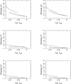 |
Fig. 5. Beaming factors (Sloan passbands) according to Eq. (4) for log g = 7.0. Continuous lines indicate LTE DA models and stars indicate NLTE DA models. |
Concerning the ATLAS9 models, Figure 6 shows the beaming factors for the Kepler, TESS, and Gaia passbands for models on the main sequence (solar metallicity, stars) and DA white dwarf models, denoted by continuous lines for a fixed value of log g = 5.0. In general, the differences are not very large because we are dealing with relatively long wavelengths. The situation changes for the ultraviolet range. In Fig. 2, we show the behavior of beaming factors of the same models as in Fig. 6 but for the u′ filter; the differences are notable in magnitude, in addition to being systematically offset. The systematic effects illustrated in Fig. 2 are due to the fact that the respective codes adopt different equations of state and helium content.
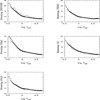 |
Fig. 6. Beaming factors for main sequence ATLAS9 models (solar metallicity, stars) and DA models (continuous lines) according to Eq. (4). All models are at log g = 5.0 and shown for the Kepler, TESS and Gaia Gbp, G, and Grp passbands. |
The comparison between theoretical and semi-empirical beaming factors is a difficult task mainly due to the scarcity of observational data. Here we analyze the semi-empirical beaming data related to white dwarfs in the passband g′, published by Shporer et al. (2010). These authors, analyzing the system NLTT 11748, a non-interacting eclipsing double white dwarf binary with optical light dominated by an extremely low mass (ELM) DA white dwarf, determined  = 3.0 ± 0.4. The system consists of He-core and C/O-core white dwarfs but both atmospheres are pure hydrogen. We present in Fig. 7 an exploratory comparison between the theoretical predictions for the passband g′ and the value inferred in Shporer et al. (2010). The theoretical beaming compares well with the derived semi-empirical value. On the other hand, Bloemen et al. (2011), studying the KPD 1946 + 4340 system, observationally determined
  = 1.33 ± 0.02 for the sdB star. Since we did not calculate the beaming factors specifically for sdB-type stars, we used the results of DA and DB models to compare. Although this comparison is not entirely consistent, it can provide us with some clues. The respective values of the beaming factors are 1.34 and 1.32 and are in agreement with the semi-empirical value given by Bloemen et al. (2011).
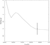 |
Fig. 7. Comparison between the semi-empirical beaming factor (error bars) for the system NLTT 11748 for the g′ passband and theoretical predictions adopting DA models at log g = 6.5. |
The beaming factor calculations for stars on the main sequence or the giant branch are also scarce in the literature. Bloemen et al. (2012), for example, present the calculation of the beaming factor for an A-type main-sequence star (KOI-74) in the Kepler passband and find  = 2.22 ± 0.04. An inspection in our Table 9 (see Table A.1) shows that the value of the beaming factor for the ATLAS9 model (Teff = 9500 K, log g = 4.3, and solar metallicity) is around 2.21, in good agreement with both the value mentioned above and the semi-empirical value (2.24 ± 0.05).
3. Limb-darkening coefficients for DA-3D and DB-3D models
Claret et al. (2020) derived LDCs for a set of one-dimensional DA, DB, and DBA white dwarf models. Here we compare these results to 3D model atmospheres for DA white dwarfs (DA-3D; Tremblay et al. 2013) in the ranges log g = 7.0–9.0 and Teff = 6000–15 000 K, and for DB/DBA white dwarfs (DBA-3D; Cukanovaite 2018, 2019 in the ranges log g = 7.5–9.0 and Teff = 12 000–34 000 K. As usual, we adopted the following limb-darkening laws for the DA-3D and DB-3D models: the linear law (Schwarzschild 1906; Russell 1912; Milne 1921)
 (5)
(5)
the quadratic law (Kopal 1950)
 (6)
(6)
the square-root law (Díaz-Cordovés & Giménez 1992)
 (7)
(7)
the logarithmic law (Klinglesmith & Sobieski 1970)
 (8)
(8)
the power-2 law (Hestroffer 1997)
 (9)
(9)
and a four-term law (Claret 2000)
 (10)
(10)
where I(1) is the specific intensity at the center of the disk and u, a, b, c, d, e, f, g, h, and ak are the corresponding LDCs. For the calculation of the LDCs, we adopted the least-squares method (LSM). For details regarding this choice, see Claret et al. (2020).
The merit function for each law and passband is given by
 (11)
(11)
where yi is the model intensity at point i, Yi is the fitted function at the same point, and N is the number of μ points. The χ2 are given in Tables 11–34 (see Appendix A) for user orientation for each law and passband.
The advantages of the four-term law over all bi-parametric or linear laws are widely discussed in Claret (2000) for main sequence and giant stars, and for the case of white dwarfs in Claret et al. (2020). In the case of 3D models for main sequence stars and giants, a discussion on the superiority of the four-term law can be found in Magic et al. (2015). In the case of the DA-3D and DB-3D models, the corresponding difference in χ2 between the six laws gives similar results to those obtained in the aforementioned papers.
In our previous paper on LDCs and GDCs for white dwarfs, we only investigated 1D models. Our main objective in this section is to study the effects of 3D models on LDCs and GDCs. However, for the calculation of the GDCs, we need to calculate the term  , where Io(λ) is the specific intensity at a given wavelength at the center of the stellar disk and the subscript Teff denotes a derivative at constant effective temperature. The impact of this contribution to the GDC is not very large, but it is not negligible. Unfortunately, the present 3D grids are not regular with respect to effective temperatures, which prevents us from performing consistent calculations of GDCs. We will address these calculations in the future, since they require an enormous amount of personal and computational time. However, we can calculate the GDCs for an individual system upon request from interested parties.
Before analyzing the LDCs for the white dwarfs, we will note that a very important but sometimes overlooked point is that a close binary system should not be treated as if each star in the pair behaves as an isolated star, since the proximity effects can change the individual properties of each star. For example, mutual irradiation between the components alters the spectra, occasionally resulting in a very different spectrum from a non-irradiated white dwarf. This can alter the distribution of specific intensities (limb-darkening), effective temperatures, and even the observed chemical compositions. In many cases, this type of interaction can lead to erroneous determinations of the stellar parameters as indicated by Claret & Giménez (1990, 1992) and Claret (2001, 2004, 2007). In this section, we work with the hypothesis that the stars in a close binary system behave like isolated stars, but we plan to implement the proximity effects in the future.
In Fig. 8, we compare the behavior of the specific intensities as a function of μ for the one- and three-dimensional DA models with Teff = 6000 K and log g = 8.0 (HiPERCAM). We note that the effective temperature is not exactly the same as the Teff of the 3D model, which is 5998 K. However, this difference is essentially negligible for comparison purposes. Examining Fig. 8, we can see a general trend that the 1D model is brighter than the corresponding 3D model toward the limb for all passbands of the HiPERCAM instrumental system. Such an effect has been previously noted by Magic et al. (2015) when these authors compared the distribution of intensities for the ATLAS (1D) and Stagger (3D) models of main sequence stars. We also find that this effect depends on the local gravity: the larger the log g, the smaller the effect, provided the other parameters of the input physics are fixed. An explanation for this effect may be that the temperature stratification and temperature gradients are different in the 1D and 3D modeling Magic et al. (2015). One contribution that changes the temperature stratification for DA and DB white dwarfs is the convective overshoot seen in 3D models, which cools the upper layers (Tremblay et al. 2013; Cukanovaite 2018). Since regions toward the limb have a longer optical path across the overshoot region, they become less bright in 3D.
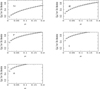 |
Fig. 8. Distribution of specific intensities for 1D (continuous line) and 3D (crosses) DA models with Teff = 6000 K and log g = 8.0 for the HiPERCAM instrumental system. |
On the other hand, as is widely known, the linear approximation for limb-darkening does not correctly describe the distribution of specific intensities. However, this law allows us to more easily compare the results from models with different input physics. We will use it here for the purpose of studying the direct effects of 3D on LDCs. Comparisons of the LDCs between DA-1D and DA-3D models are shown in Fig. 9 (HiPERCAM). Significant differences can only be distinguished for shorter effective wavelengths and lower effective temperatures, and these could be at the limit of observational detection. Three-dimensional effects due to convective energy transport become significant at low Teff and thus the differences between 1D and 3D at these temperatures are not unexpected.
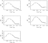 |
Fig. 9. Comparison between linear LDCs for HiPERCAM passbands for DA-3D models (crosses) and DA-1D models (continuous line) at log g = 7.0. |
In Fig. 10, we compare the linear LDCs for DB-3D models (stars) with their 1D counterparts. There is a systematic effect in the sense that the LDCs of the 3D models are smaller for Teff < 20 000 K. Similarly to DA white dwarfs, 3D effects become significant in this temperature regime (Cukanovaite 2018).
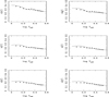 |
Fig. 10. Comparison between linear LDCs and Sloan passbands for DB-3D models (stars) and DB-1D models (continuous line) at log g = 8.0. |
According to the results shown in Fig. 8, the distribution of specific intensities for 3D models indicates that, in general, these models are less bright than their 1D counterparts, which implies steeper profiles toward the limb. To better describe these intensities, we recommend the use of the four-term law given the level of precision that is being achieved with Earth-based instruments as well as space missions, such as Kepler, TESS, and, in the near future, PLATO.
4. Summary
The beaming factor calculations presented here, based on more realistic atmosphere models, clearly indicate that the black body approximation is not accurate. This is particularly important for the filters u, u′, U, g, g′, and B since the black body approach is only valid for high effective temperatures and/or long effective wavelengths. To check the validity of our calculations of beaming factors, we compared them with the few existing cases in the literature (theoretical and semi-empirical), finding a very good agreement. To more accurately analyze the light curves of white dwarfs, we recommend the use of the beaming factors presented here. On the other hand, concerning limb-darkening, we recommend the use of the 3D four-term law since Hayek et al. (2012) has shown that 3D models lead to a better fit for the HD 189733 system when compared to the predictions of the 1D models. Finally, Tables A.1 and A.2 give information on the data available at the CDS (Centre de Données Astronomiques de Strasbourg) or directly from the authors.
Acknowledgments
We thank the referee S. Bloemen for his helpful suggestions and comments. The Spanish MEC (ESP2017-87676-C5-2-R, PID2019-107061GB-C64, and PID2019-109522GB-C52) is gratefully acknowledged for its support during the development of this work. A. C. also acknowledges financial support from the State Agency for Research of the Spanish MCIU through the “Center of Excellence Severo Ochoa” award for the Instituto de Astrofísica de Andalucía (SEV-2017-0709). The research leading to these results has received funding from the European Research Council under the European Union’s Horizon 2020 research and innovation programme n. 677706 (WD3D). SGP acknowledges the support of a Science and Technology Facilities Council (STFC) Ernest Rutherford Fellowship. This research has made use of the SIMBAD database, operated at the CDS, Strasbourg, France, and of NASA’s Astrophysics Data System Abstract Service.
References
- Bloemen, S. 2015, High-Precision Studies of Compact Variable Stars (Springer Theses) [Google Scholar]
- Bloemen, S., Marsh, T. R., Ostensen, R. H., et al. 2011, MNRAS, 410, 1787 [Google Scholar]
- Bloemen, S., Marsh, T. R., Degroote, P., et al. 2012, MNRAS, 422, 2600 [Google Scholar]
- Castelli, A., Gratton, R. G., & Kurucz, R. L. 1997, A&A, 324, 432 [Google Scholar]
- Claret, A. 2000, A&A, 363, 1081 [NASA ADS] [Google Scholar]
- Claret, A. 2001, MNRAS, 327, 989 [Google Scholar]
- Claret, A. 2004, A&A, 422, 66 [Google Scholar]
- Claret, A. 2007, A&A, 470, 1099 [NASA ADS] [CrossRef] [EDP Sciences] [Google Scholar]
- Claret, A., & Giménez, A. 1990, A&A, 230, 412 [Google Scholar]
- Claret, A., & Giménez, A. 1992, A&A, 256, 572 [NASA ADS] [Google Scholar]
- Claret, A., Cukanovaite, E., Burdge, K., et al. 2020, A&A, 634, A93 [EDP Sciences] [Google Scholar]
- Cukanovaite, E., et al. 2018, MNRAS, 481, 1522 [Google Scholar]
- Cukanovaite, E., et al. 2019, MNRAS, 490, 1010 [Google Scholar]
- Díaz-Cordovés, J., & Giménez, A. 1992, A&A, 259, 227 [NASA ADS] [Google Scholar]
- Ehrenreich, D., Lagrange, A.-M., Bouchy, F., et al. 2011, A&A, 525, A85 [NASA ADS] [CrossRef] [EDP Sciences] [Google Scholar]
- Gianninas, A., Strickland, B. D., Kilic, M., & Bergeron, P. 2013, ApJ, 765, 102 [Google Scholar]
- Hayek, W., Sing, D., & Pont, A. M. 2012, A&A, 539, A102 [NASA ADS] [CrossRef] [EDP Sciences] [Google Scholar]
- Hestroffer, D. 1997, A&A, 327, 199 [NASA ADS] [Google Scholar]
- Hills, J. G., & Dale, T. M. 1974, A&A, 30, 135 [NASA ADS] [Google Scholar]
- Klinglesmith, D. A., & Sobieski, S. 1970, AJ, 75, 175 [Google Scholar]
- Kopal, Z. 1950, HarCi, 454, 1 [Google Scholar]
- Loeb, A., & Gaudi, B. S. 2003, ApJ, 588, L117 [Google Scholar]
- Magic, Z., Chiavassa, A., Collet, R., & Asplund, M. 2015, A&A, 573, A90 [NASA ADS] [CrossRef] [EDP Sciences] [Google Scholar]
- Mazeh, T., & Faigler, S. 2010, A&A, 521, A59 [NASA ADS] [CrossRef] [EDP Sciences] [Google Scholar]
- Milne, E. A. 1921, MNRAS, 81, 361 [Google Scholar]
- Neckel, H., & Labs, D. 1994, SoPh, 153, 91N [Google Scholar]
- Pereira, T. M. D., Asplund, M., Collet, R., et al. 2013, A&A, 554, A118 [NASA ADS] [CrossRef] [EDP Sciences] [Google Scholar]
- Pierce, A. K., & Slaughter, C. D. 1977, Soph, 51, 25 [Google Scholar]
- Russell, H. N. 1912, ApJ, 36, 54 [Google Scholar]
- Shakura, N. I., & Postnov, A. 1987, A&A, 183, L21 [Google Scholar]
- Schwarzschild, K. 1906, Nachr. Ges. Wiss. Gottingen Math.-Phy. Kl., 43 [Google Scholar]
- Shporer, A., Kaplan, D. L., Steinfadt, J. D. R., et al. 2010, ApJ, 725, L200 [Google Scholar]
- Tremblay, P.-E., Ludwig, H.-G., Steffen, M., & Freytag, B. 2013, A&A, 559, A104 [NASA ADS] [CrossRef] [EDP Sciences] [Google Scholar]
- Wong, I., Shporer, A., Becker, J. C., et al. 2020, AJ, 159, 29 [Google Scholar]
Appendix A: Brief description of online data
Tables A.1 and A.2 summarize the types of data available as well as the central intensities for each photometric system in ergs cm−2 s−1 Hz−1 ster−1 in the case of LDCs for the 3D models. For more details, see the ReadMe file at the CDS website.
Doppler beaming factors for the Kepler, TESS, Gaia, HiPERCAM, Sloan, and UBVRI photometric systems.
Limb-darkening coefficients for the Kepler, TESS, Gaia, HiPERCAM, Sloan, and UBVRI photometric systems.
All Tables
Doppler beaming factors for the Kepler, TESS, Gaia, HiPERCAM, Sloan, and UBVRI photometric systems.
Limb-darkening coefficients for the Kepler, TESS, Gaia, HiPERCAM, Sloan, and UBVRI photometric systems.
All Figures
|
Fig. 1. Comparison between the beaming factors according to Eq. (4) (HiPERCAM passbands). The DA white dwarf models are represented by continuous lines and black body approximation by stars. All models are at log g = 5.0. |
| In the text | |
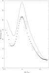 |
Fig. 2. Same as in Fig. 6 but for the u′ passband. |
| In the text | |
|
Fig. 3. Comparison between the beaming factors (Sloan passbands, DA white dwarf models) according to Eq. (4). Continuous lines indicate models with log g = 5.0 while stars denote those with log g = 9.0. |
| In the text | |
|
Fig. 4. Beaming factors for the UBVRI passbands according to Eq. (4) for log g = 5.0. Continuous lines indicate DA white dwarf models while stars denote DB models. |
| In the text | |
|
Fig. 5. Beaming factors (Sloan passbands) according to Eq. (4) for log g = 7.0. Continuous lines indicate LTE DA models and stars indicate NLTE DA models. |
| In the text | |
|
Fig. 6. Beaming factors for main sequence ATLAS9 models (solar metallicity, stars) and DA models (continuous lines) according to Eq. (4). All models are at log g = 5.0 and shown for the Kepler, TESS and Gaia Gbp, G, and Grp passbands. |
| In the text | |
|
Fig. 7. Comparison between the semi-empirical beaming factor (error bars) for the system NLTT 11748 for the g′ passband and theoretical predictions adopting DA models at log g = 6.5. |
| In the text | |
|
Fig. 8. Distribution of specific intensities for 1D (continuous line) and 3D (crosses) DA models with Teff = 6000 K and log g = 8.0 for the HiPERCAM instrumental system. |
| In the text | |
|
Fig. 9. Comparison between linear LDCs for HiPERCAM passbands for DA-3D models (crosses) and DA-1D models (continuous line) at log g = 7.0. |
| In the text | |
|
Fig. 10. Comparison between linear LDCs and Sloan passbands for DB-3D models (stars) and DB-1D models (continuous line) at log g = 8.0. |
| In the text | |
Current usage metrics show cumulative count of Article Views (full-text article views including HTML views, PDF and ePub downloads, according to the available data) and Abstracts Views on Vision4Press platform.
Data correspond to usage on the plateform after 2015. The current usage metrics is available 48-96 hours after online publication and is updated daily on week days.
Initial download of the metrics may take a while.