| Issue |
A&A
Volume 641, September 2020
|
|
|---|---|---|
| Article Number | A80 | |
| Number of page(s) | 9 | |
| Section | Planets and planetary systems | |
| DOI | https://doi.org/10.1051/0004-6361/202038372 | |
| Published online | 11 September 2020 | |
Binary asteroid (31) Euphrosyne: ice-rich and nearly spherical★,★★
1
European Southern Observatory (ESO),
Alonso de Cordova 3107,
1900
Casilla Vitacura,
Santiago, Chile
e-mail: byang@eso.org
2
Institute of Astronomy, Faculty of Mathematics and Physics, Charles University,
V Holešovičkách 2,
18000
Prague, Czech Republic
3
Université Côte d’Azur, Observatoire de la Côte d’Azur, CNRS,
Laboratoire Lagrange, France
4
Aix Marseille Univ., CNRS, LAM, Laboratoire d’Astrophysique de Marseille,
Marseille, France
5
IMCCE, Observatoire de Paris, PSL Research University, CNRS, Sorbonne Universités, UPMC Univ Paris 06, Univ. Lille, France
6
Department of Earth, Atmospheric and Planetary Sciences, MIT,
77 Massachusetts Avenue,
Cambridge,
MA
02139, USA
7
Mathematics and Statistics, Tampere University,
33014
Tampere, Finland
8
Space sciences, Technologies and Astrophysics Research Institute, Université de Liège,
Allée du 6 Août 17,
4000
Liège, Belgium
9
Astronomical Observatory Institute, Faculty of Physics, Adam Mickiewicz University,
ul. Słoneczna 36,
60-286
Poznań, Poland
10
SETI Institute, Carl Sagan Center,
189 Bernado Avenue,
Mountain View,
CA
94043, USA
11
Oukaimeden Observatory, High Energy Physics and Astrophysics Laboratory, Cadi Ayyad University,
Marrakech, Morocco
12
Thirty-Meter-Telescope,
100 West Walnut St, Suite 300,
Pasadena,
CA
91124, USA
13
Jet Propulsion Laboratory, California Institute of Technology,
4800 Oak Grove Drive,
Pasadena,
CA
91109, USA
14
European Space Agency, ESTEC – Scientific Support Office, Keplerlaan 1,
Noordwijk
2200 AG, The Netherlands
15
DOTA, ONERA, Université Paris Saclay,
F-91123
Palaiseau, France
16
Open University, School of Physical Sciences, The Open University,
MK7 6AA, UK
17
Laboratoire Atmosphères, Milieux et Observations Spatiales, CNRS & Université de Versailles Saint-Quentin-en-Yvelines,
Guyancourt, France
18
Sección Física, Departamento de Ciencias, Pontificia Universidad Católica del Perú,
Apartado 1761,
Lima, Peru
19
Departamento de Fisica, Ingeniería de Sistemas y Teoría de la Señal, Universidad de Alicante,
Alicante,
Spain
20
Institut de Ciéncies del Cosmos (ICCUB), Universitat de Barcelona (IEEC-UB),
Martí Franqués 1,
E08028
Barcelona, Spain
21
Astronomical Institute of Romanian Academy,
5, Cutitul de Argint Street,
040557
Bucharest, Romania
Received:
7
May
2020
Accepted:
15
July
2020
Aims. Asteroid (31) Euphrosyne is one of the biggest objects in the asteroid main belt and it is also the largest member of its namesake family. The Euphrosyne family occupies a highly inclined region in the outer main belt and contains a remarkably large number of members, which is interpreted as an outcome of a disruptive cratering event.
Methods. The goals of this adaptive-optics imaging study are threefold: to characterize the shape of Euphrosyne, to constrain its density, and to search for the large craters that may be associated with the family formation event.
Results. We obtained disk-resolved images of Euphrosyne using SPHERE/ZIMPOL at the ESO 8.2 m VLT as part of our large program (ID: 199.C-0074, PI: Vernazza). We reconstructed its 3D shape via the ADAM shape modeling algorithm based on the SPHERE images and the available light curves of this asteroid. We analyzed the dynamics of the satellite with the Genoid meta-heuristic algorithm. Finally, we studied the shape of Euphrosyne using hydrostatic equilibrium models.
Conclusions. Our SPHERE observations show that Euphrosyne has a nearly spherical shape with the sphericity index of 0.9888 and its surface lacks large impact craters. Euphrosyne’s diameter is 268 ± 6 km, making it one of the top ten largest main belt asteroids. We detected a satellite of Euphrosyne – S/2019 (31) 1 – that is about 4 km across, on a circular orbit. The mass determined from the orbit of the satellite together with the volume computed from the shape model imply a density of 1665 ± 242 kg m−3, suggesting that Euphrosyne probably contains a large fraction of water ice in its interior. We find that the spherical shape of Euphrosyne is a result of the reaccumulation process following the impact, as in the case of (10) Hygiea. However, our shape analysis reveals that, contrary to Hygiea, the axis ratios of Euphrosyne significantly differ from those suggested by fluid hydrostatic equilibrium following reaccumulation.
Key words: techniques: high angular resolution / methods: observational / minor planets, asteroids: individual: (31) Euphrosyne / minor planets, asteroids: general
The reduced images are only available at the CDS via anonymous ftp to cdsarc.u-strasbg.fr (130.79.128.5) or via http://cdsarc.u-strasbg.fr/viz-bin/cat/J/A+A/641/A80
© ESO 2020
1 Introduction
The main asteroid belt is a dynamically living relic, in which the shapes, sizes, and surfaces of most asteroids are altered by ongoing collisional fragmentation and cratering events (Bottke et al. 2015). Space probes and ground-based observations have revealed a fascinating variety among asteroid shapes; large asteroids are nearly spherical (Park et al. 2019; Vernazza et al. 2020) and small asteroids are irregularly shaped (Ďurech et al. 2010; Shepard et al. 2017; Fujiwara et al. 2006; Thomas et al. 2012). Most asteroids with diameters greater than ~100 km have likely kept their internal structure intact since their time of formation because the dynamical lifetime of those asteroids is estimated to be comparable to the age of the solar system (Bottke et al. 2005). There are a few exceptions essentially comprising the largest remnants of asteroid families (e.g., (10) Hygiea; Vernazza et al. 2020), whose shapes have largely been altered by the impact. In contrast, the shapes of smaller asteroids have been determined mainly through collisions, where their final shapes depend on collision conditions such as impact energies and spin rates (Leinhardt et al. 2000; Sugiura et al. 2018).
The arrival of second generation extreme adaptive-optics (AO) instruments, such as the Spectro-Polarimetric High-contrast Exoplanet Research instrument (SPHERE) at the Very Large Telescope (VLT; Beuzit et al. 2008) and the Gemini Planet Imager (GPI) at GEMINI-South (Macintosh et al. 2014), offers a great opportunity to study the detailed shape, precise size, and topographic features of large main belt asteroids with diameter D ≥ 100 km via direct imaging. Observations aided by AO with high spatial resolution also enable the detection of asteroidal satellites that are much smaller and closer to their primaries, which have thus far remained undetected in prior searches (Margot et al. 2015). Consequently, physical properties that are not well constrained, such as bulk density, internal porosity, and surface tensile strength, can be investigated using AO-corrected measurements. These are the main parameters that determine crater formation, family formation, and satellite creation (Michel et al. 2001).
Asteroid (31) Euphrosyne (hereafter, Euphrosyne) is the largest member of its namesake family. Previous studies have noted that the Euphrosyne family exhibits a very steep size frequency distribution (SFD), which is significantly depleted in large- and medium-sized asteroids (Carruba et al. 2014). Such a steep SFD is interpreted as a glancing impact between two large bodies resulting in a disruptive cratering event (Masiero et al. 2015). Euphrosyne is a Cb-type asteroid (Bus & Binzel 2002) with an optical albedo of pV = 0.045 ± 0.008 (Masiero et al. 2013). Euphrosyne’s diameter has been reported as D = 276 ± 3 km (Usui et al. 2011) or D = 282 ± 10 km (Masiero et al. 2013), while its mass has been estimated by various studies leading to an average value of M31 = 1.27 ± 0.65 × 10¹⁹ kg with about 50% uncertainty (Carry 2012). These size and mass estimates imply a density estimate of ρ31 = 1180 ± 610 kg m−3. As detailed hereafter and first reported in (CBET 4627, 2019), we discovered a satellite in this study, implying that it is one of the few large asteroids for which the density can be constrained with high precision (Scheeres et al. 2015).
In this paper, we present the high-angular resolution observations of Euphrosyne with VLT/SPHERE/ZIMPOL, which were obtained as part of our ESO large program (Sect. 2.1). We use these observations, together with a compilation of available and newly obtained optical light curves (Sect. 2.2), to constrain the 3D shape of Euphrosyne as well as its spin state and surface topography (Sect. 3). We then describe the discovery of its small moonlet S/2019 (31) 1 (Sect. 4) and constrain its mass by fitting the orbit of the satellite. Both the 3D shape (hence volume) and the mass estimate allow us to constrain the density of Euphrosyne with high precision (Sect. 5). We also use the AO images and the 3D shape model to search for large craters, which may be associated with the family-forming event.
2 Observations and data reduction
2.1 Disk-resolved data with SPHERE
Euphrosyne was observed, between March and April 2019, using the Zurich Imaging Polarimeter (ZIMPOL) of SPHERE (Thalmann et al. 2008) in the direct imaging mode with the narrow band filter (N_ R filter; filter central wavelength = 645.9 nm, width = 56.7 nm). The angular diameter of Euphrosyne was in the range 0.16–0.17′′ and the asteroid was close to an equator-on geometry at the time of the observations. Therefore, the SPHERE images of Euphrosyne obtained from seven epochs allowed us to reconstruct a reliable 3D shape model with well-defined dimensions. The reduced images were further deconvolved with the Mistral algorithm (Fusco et al. 2003), using a parametric point-spread function (Fétick et al. 2019). Table A.1 contains full information about the images. We represent the obtained images in Fig. A.1.
2.2 Disk-integrated optical photometry
A set of 29 individual light curves of Euphrosyne was previously used by Hanuš et al. (2016a) in order to derive a convex shape model of this large body. These light curves were obtained from the previous studies (Schober et al. 1980; Barucci et al. 1985; McCheyne et al. 1985; Kryszczynska et al. 1996; Pilcher & Jardine 2009; Pilcher 2012). We complemented these data with five additional light curves from the recent apparition in 2017. Four light curves were obtained by the TRAPPIST North telescope (Fig. 1) and the fifth was obtained via the Gaia-GOSA1. Our final photometric data set utilized for the shape modeling of Euphrosyne consists of 34 individual light curves. Detailed information about these light curves is provided in Table A.2
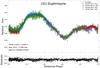 |
Fig. 1 Composite light curve of (31) Euphrosyne obtained with the TRAPPIST-North telescope in 2017 and a Fourier series of fifth order is fitted to the data, shown as the solid line. The residuals of the fit are shown as black dots below. The details about the telescope and data format are described in Jehin et al. (2011). |
3 Determination of the 3D shape
The spin state solution from Hanuš et al. (2016a) served as an initial input for the shape modeling with the All-data Asteroid Modeling algorithm (ADAM ; Viikinkoski et al. 2015a), which simultaneously fits the optical data and disk-resolved images. We followed the same shape modeling approach applied in our previous studies based on disk-resolved data from the SPHERE large program (e.g., Vernazza et al. 2018; Viikinkoski et al. 2018; Hanuš et al. 2019). First, we constructed a low-resolution shape model basedon all available data; we subsequently used this shape model as a starting point for further modeling with decreased weight of the light curves and increased shape model resolution. We performed this approach iteratively until we were satisfied with the fit to the light curve and disk-resolved data. We also tested two different shape parametrizations: octantoids and subdivision (Viikinkoski et al. 2015a). We show the comparison between the VLT/SPHERE/ZIMPOL deconvolvedimages of Euphrosyne and the corresponding projections of the shape model in Fig. 2.
Owing to the nearly equator-on geometry of the asteroid, our images taken at seven different rotation phases have a nearly complete coverage of the entire surface of Euphrosyne. The SPHERE data enable an accurate determination of Euphrosyne’s dimensions, including those along the rotation axis. The physical properties of Euphrosyne derived are listed in Table 1. The uncertainties reflect the dispersion of values obtained with various shape models based on different data weighting, shape resolution, and parametrization. These values correspond to about 1 pixel, which is equivalent to ~5.93 km. Our volume equivalent diameter D = 268 ± 6 km is consistent within 1σ with the radiometric estimates of Usui et al. (2011; D = 276 ± 3 km) and Masiero et al. (2013; D = 282 ± 10 km). The shape of Euphrosyne is fairly spherical with almost equal equatorial dimensions (a∕b = 1.05 ± 0.03) and only a small flattening (b∕c = 1.13 ± 0.04) along the spin axis. Euphrosyne’s sphericity index (see Vernazza et al. 2020 for more details) is equal to 0.9888, which is somewhat higher than that of (4) Vesta, (2) Pallas, and (704) Interamnia (Vernazza et al. 2020; Hanuš et al. 2020), making it so far the third most spherical main belt asteroid after Ceres and Hygiea.
Given the rather spherical shape of Euphrosyne and the fact that its a and b axes have similar lengths (within errors), we investigated whether the shape of Euphrosyne is close to hydrostatic equilibrium, using the same approach as described in Hanuš et al. (2020). It appears that Euphrosyne’s shape is significantly different from the Maclaurin spheroid, which would be much flatter along the c axis (see Fig. 3). Our SPHERE observations show that Euphrosyne is not in hydrostatic equilibrium for its current rotation, which is discussed further in Sect. 6.
 |
Fig. 2 Comparison between the VLT/SPHERE/ZIMPOL deconvolved images of Euphrosyne (bottom) and the corresponding projections of our ADAM shape model (top). The red line indicates the position of the rotation axis. A non-realisticillumination highlights the local topography of the model. |
Physical properties of (31) Euphrosyne based on ADAM shape modeling and the Genoid orbit solution of the satellite: sidereal rotation period P, spin-axis ecliptic J2000 coordinates λ and β, volume-equivalent diameter D, dimensions along the major axis a, b, c, their ratios a∕b and b∕c, mass M, and bulk density ρ.
4 Orbital properties of the satellite
Each image obtained with SPHERE/ZIMPOL was further processed to remove the bright halo surrounding Euphrosyne, following the procedure described in details in Pajuelo et al. (2018) and Yang et al. (2016). The residual structures after the halo removal were minimized using the processing techniques introduced in Wahhaj et al. (2013), where the background structures were removed using a running median in a ~50 pixel box in the azimuthal direction as well as in a ~40 pixel box in the radial direction. Adopting the method introduced in Yang et al. (2016), we inserted 100 point sources, with known intensities and full width at half maximum (FWHM), in each science image to estimate flux loss due to the halo removal processes. In five out of seven epochs, a faint non-resolved source was clearly detected in the vicinity of Euphrosyne (Fig. 4). The variation in the brightness of the satellite is mainly due to the difference in the atmospheric conditions at the time of the observations, which directly affects the AO performance.
We measured the relative positions on the plane of the sky between Euphrosyne and its satellite (fitting two 2D Gaussians; see Carry et al. 2019) and report these in Table B.1. We then used the Genoid algorithm (Vachier et al. 2012) to determine the orbital elements of the satellite. The best solution fits the observed positions with root mean square (RMS) residuals of only 1.5 mas (Table 2). The orbit of the satellite is circular, prograde, and equatorial, similar to most known satellites around large main belt asteroids (e.g., Marchis et al. 2008; Berthier et al. 2014; Margot et al. 2015; Carry et al. 2019).
From the difference in the apparent magnitude of 9.0 ± 0.3 between Euphrosyne and S/2019 (31) 1, and assuming a similar albedo for both, we estimated the diameter of the satellite to be 4.0 ±1.0 km. The Euphrosyne binary system has a relative component separation of a∕RP = 5.0 ± 0.3 and a secondary-to-primary diameter ratio Ds∕Dp = 0.015 ± 0.005, where a is the semimajor axis of the system, Ds and Dp are the diameter of the satellite and the primary respectively, and RP is the radiusof the primary. The comparison of the properties of the Euphrosyne binary system to other large asteroid systems are shown in Fig. 5. Compared to the other systems, S/2019 (31) 1 has one of the smallest secondary-to-primary diameter ratios and is very close to the primary. Given the small size of the satellite, S/2019 (31) is expected to be tidally locked, that is, its spin period synchronizes to its orbital period on a million year timescale (Rojo & Margot 2011).
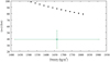 |
Fig. 3 Calculated (a–c) for (31) Euphrosyne as function of mean density for homogeneous case, given Euphrosyne’s rotation period of 5.53h, shown as black dots. The green star represents the value derived in Sect. 5 with its 1σ uncertainty (uncertainties of a and c are added quadratically). |
 |
Fig. 4 Processed ZIMPOL images, revealing the presence of the satellite, S/2019 (31) 1, around (31) Euphrosyne in five epochs. The pixel intensities within 0.22″ of the primary are reduced by a factor of ~2000 to increase the visibility of the faint satellite. The images are smoothed by convolving a Gaussian function with FWHM of ~8 pixels. |
Orbital elements of the satellite of Euphrosyne, expressed in EQJ2000, obtained with Genoid : orbital period P, semimajor axis a, eccentricity e, inclination i, longitude of the ascending node Ω, argument of pericenter ω, and time of pericenter tp.
5 Bulk density and surface topography
Owing to the presence of the satellite, we derived the mass of the system (1.7 ± 0.3) × 1019 kg with a fractional precision of 15%, which is considerably better than all the previous indirect measurements. Combining our mass measurement with the newly derived volume based on our 3D shape, we obtained a bulk density of 1.665± 0.242 g cm−3 for Euphrosyne.
We note that the bulk density of Euphrosyne is the lowest among all the other large C-type asteroids measured to date; these include (1) Ceres (2.161 ± 0.003 g cm−3, D ~ 1000 km; Park et al. 2019), (10) Hygiea (1.94 ± 0.25 g cm−3, D ~ 440 km; Vernazza et al. 2020), and (704) Interamnia (1.98 ± 0.68 g cm−3, D ~ 300 km; Hanuš et al. 2020). On the other hand, such density around 1.7 g cm−3 or lower is more common among intermediate-sized C-type asteroids, such as (45) Eugenia (1.4 ± 0.4 g cm−3, D ~ 200 km; Marchis et al. 2012), (93) Minerva (1.75 ± 0.68 g cm−3, D ~ 160 km, Marchis et al. 2013), (130) Eletra (1.60 ± 0.13 g cm−3, D ~ 200 km; Hanuš et al. 2016b), and (762) Pulcova (0.8 ± 0.1 g cm−3, D ~ 150 km; Marchis et al. 2012).
For the C-complex asteroids mentioned above, the density seems to show a trend with size, where the smaller asteroids have lower densities. This trend could be explained by increasing porosity in smaller asteroids. Nonetheless, as already discussed in recent works (Carry 2012; Viikinkoski et al. 2015b; Marsset et al. 2017; Carry et al. 2019; Hanuš et al. 2020), the macroporosity of Euphrosyne is likely to be small (≤20%) because of its relatively high internal pressure due to its large mass > 1019kg. Given the small macroporosity of Euphrosyne, its density, therefore, is diagnostic of its bulk composition. As for the other large C-type asteroids (Ceres, Hygiea, Interamnia), a large amount of water must be present in Euphrosyne. Assuming 20% porosity, a typical density of anhydrous silicates of 3.4 g cm−3 and a density of 1.0 g cm−3 for water ice, the presence of water ice, up to 50% by volume, is required in the interior of Euphrosyne to match its bulk density.
In terms of topographic characteristics, the surface of Euphrosyne appears smooth and nearly featureless without any apparent large basins. This is in contrast to other objects studied by our large program that show various-sized craters on their surfaces, such as (2) Pallas (B-type; Marsset et al. 2020), (4) Vesta (V-type; Fétick et al. 2019); and (7) Iris (S-type; Hanuš et al. 2019). On the other hand, lacking surface features in AO images is not unprecedented among large asteroids, especially among C-type asteroids. Ground-based AO observations have identified at least three other cases that are lacking prominent topographic structures, namely (1) Ceres (Carry et al. 2008), (10) Hygiea (Vernazza et al. 2020), and (704) Interamnia (Hanuš et al. 2020). Although NASA/Dawn observations revealed a highly cratered surface of Ceres (Hiesinger et al. 2016), this dwarf planet clearly lacks large craters, which suggests rapid viscous relaxation or protracted resurfacing due to the presence of large amounts of water (Marchi et al. 2016).
Similarly, as previously discussed for the cases of Hygiea (Vernazza et al. 2020) and Interamnia (Hanuš et al. 2020), the absence of apparent craters in our Euphrosyne images may be due to the flat-floored shape of D ≥ 40 km craters; this diameter corresponds to the minimum size of features that can be recognized on the surface of Euphrosyne. This flat-floored shape would be consistent with a high water content for this asteroid, which agrees with our bulk density estimate.
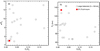 |
Fig. 5 Panel a: relative component separation and panel b: primary radius vs. secondary to primary diameter ratio for presently known main belt binary and triple asteroids (Johnston 2018). Large asteroids with diameters greater than 100 km are shown as open circles. Asteroid (90) Antiope is excluded because of its unusually large secondary to primary diameter ratio. Our measurements of (31) Euphrosyne are shown as red squares. |
6 Discussion
In an attempt to understand the unexpected nearly spherical shape of Euphrosyne, we adopted a similar approach as described in Vernazza et al. (2020) and used hydrodynamical simulations to study the family-formation event. The simulations were performed with a smoothed-particle hydrodynamics (SPH) code to constrain the impact parameters, such as the impact angle and diameter of the impactor. We assumed the target and impactor are both monolithic bodies with an initial density of the material ρ0 = 1665 kg m−3, corresponding to the present-day density of Euphrosyne. Our SPH simulations find that the impact event of Euphrosyne is even more energetic in comparison to that of Hygiea. As such, the parent body of Euphrosyne is completely fragmented by the impact and the final reaccumulated shape of Euphrosyne is highly spherical, which is similar to the case of Hygiea, where the nearly round shape is formed following post-impact reaccumulation (Vernazza et al. 2020).
We further studied the orbital evolution of the Euphrosyne family and determined the age of the family, using the newly developed method (Brož & Morbidelli 2019). Our N-body simulations further constrained the age of the Euphrosyne family to τ ~ 280 Myr that is significantly younger than the previous estimates (between 560 and 1160 Myr, Carruba et al. 2014). The details of our SPH simulation as well as a full characterization of the Euphrosyne family are presented in a forthcoming article (Yang et al. 2020). The young dynamical age and post-impact reaccumulation, collectively, may have contributed to the apparent absence of craters on the surface of Euphrosyne.
Our new finding about the young age of Euphrosyne makes this asteroid a unique object for us to study the impact aftermath on a very young body that is only ~0.3 Gyr old. Previously, the SPH simulations for the case of Hygiea showed that its shape relaxed to a sphere during the gravitational reaccumulation phase, accompanied by an acoustic fluidization. The relaxation process on Hygiea could have settled down on a timescale of a few hours (Vernazza et al. 2020). However, the shape relaxation, in theory, maybe a rather long-term process, which could possibly last as long as the age of the body (τ = 3 Gyr, as suggested by its family). If the physical mechanisms work the same way on both bodies, then the relaxation timescale simply cannot be short on one body (D = 268 km) and be ten times longer on the other, larger, body (D = 434 km). To reconcile with both observations, the shape relaxation, if it is a long-term process, should occur on a timescale that is comparable to or less than 0.3 Gyr.
In addition to the much younger dynamical age, the rotation period of Euphrosyne is also shorter (P = 5.53 h) than those of Hygiea and Ceres. As noted in Descamps et al. (2011), the spin rate of Euphrosyne is faster than the typical rotation rates of asteroids with similar sizes. This is interpreted as a result of a violent disruption process, where the parent body is reaccumulated into high angular momentum shape and spin configuration (Walsh & Jacobson 2015). With that spin rate, we would expect Euphrosyne to have a shorter c axis compared to the a axis using MacLaurin’s equation (Chandrasekhar 1969) as shown in Fig. 3. However, a MacLaurin ellipsoid represents the hydrostatic equilibrium figure of a homogeneous and intact body, which is not the case for Euphrosyne since it is a reaccumulated body. This may explain why the actual shape of Euphrosyne deviates from that of a MacLaurin ellipsoid.
7 Conclusions
In this paper, we present high angular imaging observations of asteroid (31) Euphrosyne and its moon. Our main findings are summarized as follows:
- 1)
The disk-resolved images and the 3D-shape model of Euphrosyne show that it is the third most spherical body among the main belt asteroids with known shapes after Ceres and Hygiea. Its round shape is consistent with a reaccumulation event following the giant impact at the origin of the Euphrosyne family.
- 2)
The orbit of Euphrosyne’s satellite, S/2019 (31) 1, is circular, prograde, and equatorial, that is, similar to most knownsatellites around large main belt asteroids. The estimated diameter of this newly detected satellite is 4 ± 1 km, assuming a similar albedo for the satellite and the primary.
- 3)
The bulk density of Euphrosyne is 1665 ± 242 kg m−3, which is the first high-precision density measurement via ground-based observations for a Cb type asteroid. Such density implies that a large amount of water (at least 50% in volume) must be present in Euphrosyne.
- 4)
The surface of Euphrosyne is nearly featureless with no large craters detected, which is consistent with its young age and ice-rich composition.
Acknowledgements
This work has been supported by the Czech Science Foundation through grant 18-09470S (J. Hanuš, O. Chrenko, P. Ševeček) and by the Charles University Research program No. UNCE/SCI/023. M.B. was supported by the Czech Science Foundation grant 18-04514J. Computational resources were supplied by the Ministry of Education, Youth and Sports of the Czech Republic under the projects CESNET (LM2015042) and IT4Innovations National Supercomputing Centre (LM2015070). P. Vernazza, A. Drouard, M. Ferrais and B. Carry were supported by CNRS/INSU/PNP. M.M. was supported by the National Aeronautics and Space Administration under grant No. 80NSSC18K0849 issued through the Planetary Astronomy Program. The work of TSR was carried out through grant APOSTD/2019/046 by Generalitat Valenciana (Spain). This work was supported by the MINECO (Spanish Ministry of Economy) through grant RTI2018-095076-B-C21 (MINECO/FEDER, UE). The research leading to these results has received funding from the ARC grant for Concerted Research Actions, financed by the Wallonia-Brussels Federation. TRAPPIST is a project funded by the Belgian Fonds (National) de la Recherche Scientifique (F.R.S.-FNRS) under grant FRFC 2.5.594.09.F. TRAPPIST-North is a project funded by the Université de Liège, and performed in collaboration with Cadi Ayyad University of Marrakesh. E. Jehin is a FNRS Senior Research Associate.
Appendix A Additional figures and tables
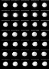 |
Fig. A.1 Full set of VLT/SPHERE/ZIMPOL images of (31) Euphrosyne. We show the images deconvolved by the Mistral algorithm. Table A.1 contains full information about the data. |
VLT/SPHERE disk-resolved images obtained in the I filter by the ZIMPOL camera.
Optical disk-integrated lightcurves used for ADAM shape modeling.
Appendix B Astrometry of the satellite
Astrometry of Euphrosyne’s satellite S/2019 (31) 1.
References
- Barucci, M. A., Fulchignoni, M., Burchi, R., & D’Ambrosio, V. 1985, Icarus, 61, 152 [NASA ADS] [CrossRef] [Google Scholar]
- Berthier, J., Vachier, F., Marchis, F., Ďurech, J., & Carry, B. 2014, Icarus, 239, 118 [NASA ADS] [CrossRef] [Google Scholar]
- Beuzit, J.-L., Feldt, M., Dohlen, K., et al. 2008, Proc. SPIE, 7014, 701418 [Google Scholar]
- Bottke, W. F., Durda, D. D., Nesvorný, D., et al. 2005, Icarus, 179, 63 [NASA ADS] [CrossRef] [Google Scholar]
- Bottke, W. F., Vokrouhlický, D., Walsh, K. J., et al. 2015, Icarus, 247, 191 [NASA ADS] [CrossRef] [Google Scholar]
- Brož, M., & Morbidelli, A. 2019, Icarus, 317, 434 [CrossRef] [Google Scholar]
- Bus, S. J., & Binzel, R. P. 2002, Icarus, 158, 146 [NASA ADS] [CrossRef] [Google Scholar]
- Carruba, V., Aljbaae, S., & Souami, D. 2014, ApJ, 792, 46 [NASA ADS] [CrossRef] [Google Scholar]
- Carry, B. 2012, Planet. Space Sci., 73, 98 [NASA ADS] [CrossRef] [Google Scholar]
- Carry, B., Dumas, C., Fulchignoni, M., et al. 2008, A&A, 478, 235 [NASA ADS] [CrossRef] [EDP Sciences] [Google Scholar]
- Carry, B., Vachier, F., Berthier, J., et al. 2019, A&A, 623, A132 [NASA ADS] [CrossRef] [EDP Sciences] [Google Scholar]
- Chandrasekhar, S. 1969, in Ellipsoidal Figures of Equilibrium (New Haven, London: Yale University Press) [Google Scholar]
- Descamps, P., Marchis, F., Berthier, J., et al. 2011, Icarus, 211, 1022 [NASA ADS] [CrossRef] [Google Scholar]
- Ďurech, J., Sidorin, V., & Kaasalainen, M. 2010, A&A, 513, A46 [NASA ADS] [CrossRef] [EDP Sciences] [Google Scholar]
- Fétick, R. J., Jorda, L., Vernazza, P., et al. 2019, A&A, 623, A6 [NASA ADS] [CrossRef] [EDP Sciences] [Google Scholar]
- Fujiwara, A., Kawaguchi, J., Yeomans, D. K., et al. 2006, Science, 312, 1330 [NASA ADS] [CrossRef] [PubMed] [Google Scholar]
- Fusco, T., Mugnier, L. M., Conan, J.-M., et al. 2003, Proc. SPIE, 4839, 1065 [NASA ADS] [CrossRef] [Google Scholar]
- Hanuš, J., Ďurech, J., Oszkiewicz, D. A., et al. 2016a, A&A, 586, A108 [NASA ADS] [CrossRef] [EDP Sciences] [Google Scholar]
- Hanuš, J., Delbo, M., Vokrouhlický, D., et al. 2016b, in AAS/Division for Planetary Sciences Meeting Abstracts, Vol. 48, AAS/Division for Planetary Sciences Meeting Abstracts, 516.08 [Google Scholar]
- Hanuš, J., Marsset, M., Vernazza, P., et al. 2019, A&A, 624, A121 [NASA ADS] [CrossRef] [EDP Sciences] [Google Scholar]
- Hanuš, J., Vernazza, P., Viikinkoski, M., et al. 2020, A&A, 633, A65 [CrossRef] [EDP Sciences] [Google Scholar]
- Hiesinger, H., Marchi, S., Schmedemann, N., et al. 2016, Science, 353, aaf4758 [NASA ADS] [CrossRef] [Google Scholar]
- Jehin, E., Gillon, M., Queloz, D., et al. 2011, The Messenger, 145, 2 [NASA ADS] [Google Scholar]
- Johnston, W. R. 2018, NASA Planetary Data System [Google Scholar]
- Kryszczynska, A., Colas, F., Berthier, J., Michałowski, T., & Pych, W. 1996, Icarus, 124, 134 [NASA ADS] [CrossRef] [Google Scholar]
- Leinhardt, Z. M., Richardson, D. C., & Quinn, T. 2000, Icarus, 146, 133 [CrossRef] [Google Scholar]
- Macintosh, B., Graham, J. R., Ingraham, P., et al. 2014, Proc. Natl. Acad. Sci. U.S.A., 111, 12661 [Google Scholar]
- Marchi, S., Ermakov, A. I., Raymond, C. A., et al. 2016, Nat. Commun., 7, 12257 [NASA ADS] [CrossRef] [Google Scholar]
- Marchis, F., Descamps, P., Baek, M., et al. 2008, Icarus, 196, 97 [NASA ADS] [CrossRef] [Google Scholar]
- Marchis, F., Enriquez, J. E., Emery, J. P., et al. 2012, Icarus, 221, 1130 [NASA ADS] [CrossRef] [Google Scholar]
- Marchis, F., Vachier, F., Ďurech, J., et al. 2013, Icarus, 224, 178 [NASA ADS] [CrossRef] [Google Scholar]
- Margot, J. L., Pravec, P., Taylor, P., Carry, B., & Jacobson, S. 2015, Asteroids IV, eds. P. Michel, F. E. DeMeo, & W. F. Bottke, (Tucson, AZ: University Arizona Press), 355–374 [Google Scholar]
- Marsset, M., Carry, B., Dumas, C., et al. 2017, A&A, 604, A64 [NASA ADS] [CrossRef] [EDP Sciences] [Google Scholar]
- Marsset, M., Brož, M., Vernazza, P., et al. 2020, Nat. Astron., 4, 569 [CrossRef] [Google Scholar]
- Masiero, J. R., Mainzer, A. K., Bauer, J. M., et al. 2013, ApJ, 770, 7 [NASA ADS] [CrossRef] [Google Scholar]
- Masiero, J. R., Carruba, V., Mainzer, A., Bauer, J. M., & Nugent, C. 2015, ApJ, 809, 179 [NASA ADS] [CrossRef] [Google Scholar]
- McCheyne, R. S., Eaton, N., & Meadows, A. J. 1985, Icarus, 61, 443 [NASA ADS] [CrossRef] [Google Scholar]
- Michel, P., Benz, W., Tanga, P., & Richardson, D. C. 2001, Science, 294, 1696 [NASA ADS] [CrossRef] [PubMed] [Google Scholar]
- Pajuelo, M., Carry, B., Vachier, F., et al. 2018, Icarus, 309, 134 [NASA ADS] [CrossRef] [Google Scholar]
- Park, R. S., Vaughan, A. T., Konopliv, A. S., et al. 2019, Icarus, 319, 812 [NASA ADS] [CrossRef] [Google Scholar]
- Pilcher, F. 2012, Minor Planet Bull., 39, 57 [Google Scholar]
- Pilcher, F., & Jardine, D. 2009, Minor Planet Bull., 36, 52 [Google Scholar]
- Rojo, P., & Margot, J. L. 2011, ApJ, 727, 69 [NASA ADS] [CrossRef] [Google Scholar]
- Scheeres, D. J., Britt, D., Carry, B., Holsapple, K. A. 2015, Asteroids IV, eds. P. Michel, F. E. DeMeo, & W. F. Bottke, (Tucson, AZ: University Arizona Press), 745 [Google Scholar]
- Schober, H. J., Scaltriti, F., Zappala, V., & Harris, A. W. 1980, A&A, 91, 1 [NASA ADS] [Google Scholar]
- Shepard, M. K., Richardson, J., Taylor, P. A., et al. 2017, Icarus, 281, 388 [NASA ADS] [CrossRef] [Google Scholar]
- Sugiura, K., Kobayashi, H., & Inutsuka, S. 2018, A&A, 620, A167 [NASA ADS] [CrossRef] [EDP Sciences] [Google Scholar]
- Thalmann, C., Schmid, H. M., Boccaletti, A., et al. 2008, Proc. SPIE, 7014, 70143F [Google Scholar]
- Thomas, N., Barbieri, C., Keller, H. U., et al. 2012, Planet. Space Sci., 66, 96 [NASA ADS] [CrossRef] [Google Scholar]
- Usui, F., Kuroda, D., Müller, T. G., et al. 2011, PASJ, 63, 1117 [NASA ADS] [CrossRef] [Google Scholar]
- Vachier, F., Berthier, J., & Marchis, F. 2012, A&A, 543, A68 [NASA ADS] [CrossRef] [EDP Sciences] [Google Scholar]
- Vernazza, P., Brož, M., Drouard, A., et al. 2018, A&A, 618, A154 [NASA ADS] [CrossRef] [EDP Sciences] [Google Scholar]
- Vernazza, P., Jorda, L., Ševeček, P., et al. 2020, Nat. Astron., 4, 136 [CrossRef] [Google Scholar]
- Viikinkoski, M., Kaasalainen, M., & Ďurech, J. 2015a, A&A, 576, A8 [NASA ADS] [CrossRef] [EDP Sciences] [Google Scholar]
- Viikinkoski, M., Kaasalainen, M., Ďurech, J., et al. 2015b, A&A, 581, L3 [NASA ADS] [CrossRef] [EDP Sciences] [Google Scholar]
- Viikinkoski, M., Vernazza, P., Hanuš, J., et al. 2018, A&A, 619, L3 [NASA ADS] [CrossRef] [EDP Sciences] [Google Scholar]
- Wahhaj, Z., Liu, M. C., Biller, B. A., et al. 2013, ApJ, 779, 80 [NASA ADS] [CrossRef] [Google Scholar]
- Walsh, K. J., & Jacobson, S. A. 2015, Asteroids IV, eds. P. Michel, F. E. DeMeo, & W. F. Bottke (Tucson, AZ: University Arizona Press), 375–393 [Google Scholar]
- Yang, B., Wahhaj, Z., Beauvalet, L., et al. 2016, ApJ, 820, L35 [NASA ADS] [CrossRef] [Google Scholar]
- Yang, B., Hanuš, J., Brož, M., et al. 2020, A&A, submitted [Google Scholar]
www.gaiagosa.eu. This web-service platform serves as a link between scientists seeking photometric data and amateur observers capable of obtaining such data with their small-aperture telescopes.
All Tables
Physical properties of (31) Euphrosyne based on ADAM shape modeling and the Genoid orbit solution of the satellite: sidereal rotation period P, spin-axis ecliptic J2000 coordinates λ and β, volume-equivalent diameter D, dimensions along the major axis a, b, c, their ratios a∕b and b∕c, mass M, and bulk density ρ.
Orbital elements of the satellite of Euphrosyne, expressed in EQJ2000, obtained with Genoid : orbital period P, semimajor axis a, eccentricity e, inclination i, longitude of the ascending node Ω, argument of pericenter ω, and time of pericenter tp.
All Figures
|
Fig. 1 Composite light curve of (31) Euphrosyne obtained with the TRAPPIST-North telescope in 2017 and a Fourier series of fifth order is fitted to the data, shown as the solid line. The residuals of the fit are shown as black dots below. The details about the telescope and data format are described in Jehin et al. (2011). |
| In the text | |
|
Fig. 2 Comparison between the VLT/SPHERE/ZIMPOL deconvolved images of Euphrosyne (bottom) and the corresponding projections of our ADAM shape model (top). The red line indicates the position of the rotation axis. A non-realisticillumination highlights the local topography of the model. |
| In the text | |
|
Fig. 3 Calculated (a–c) for (31) Euphrosyne as function of mean density for homogeneous case, given Euphrosyne’s rotation period of 5.53h, shown as black dots. The green star represents the value derived in Sect. 5 with its 1σ uncertainty (uncertainties of a and c are added quadratically). |
| In the text | |
|
Fig. 4 Processed ZIMPOL images, revealing the presence of the satellite, S/2019 (31) 1, around (31) Euphrosyne in five epochs. The pixel intensities within 0.22″ of the primary are reduced by a factor of ~2000 to increase the visibility of the faint satellite. The images are smoothed by convolving a Gaussian function with FWHM of ~8 pixels. |
| In the text | |
|
Fig. 5 Panel a: relative component separation and panel b: primary radius vs. secondary to primary diameter ratio for presently known main belt binary and triple asteroids (Johnston 2018). Large asteroids with diameters greater than 100 km are shown as open circles. Asteroid (90) Antiope is excluded because of its unusually large secondary to primary diameter ratio. Our measurements of (31) Euphrosyne are shown as red squares. |
| In the text | |
|
Fig. A.1 Full set of VLT/SPHERE/ZIMPOL images of (31) Euphrosyne. We show the images deconvolved by the Mistral algorithm. Table A.1 contains full information about the data. |
| In the text | |
Current usage metrics show cumulative count of Article Views (full-text article views including HTML views, PDF and ePub downloads, according to the available data) and Abstracts Views on Vision4Press platform.
Data correspond to usage on the plateform after 2015. The current usage metrics is available 48-96 hours after online publication and is updated daily on week days.
Initial download of the metrics may take a while.