| Issue |
A&A
Volume 641, September 2020
|
|
|---|---|---|
| Article Number | L8 | |
| Number of page(s) | 8 | |
| Section | Letters to the Editor | |
| DOI | https://doi.org/10.1051/0004-6361/202038214 | |
| Published online | 22 September 2020 | |
Letter to the Editor
Chandra X-ray study confirms that the magnetic standard Ap star KQ Vel hosts a neutron star companion⋆
1
Institute for Physics and Astronomy, University Potsdam, 14476 Potsdam, Germany
e-mail: This email address is being protected from spambots. You need JavaScript enabled to view it.
2
Department of Astronomy, Kazan Federal University, Kremlevskaya Str 18, Kazan, Russia
3
Department of Physics & Astronomy, East Tennessee State University, Johnson City, TN 37614, USA
4
NAF – Osservatorio Astrofisico di Catania, Via S. Sofia 78, 95123 Catania, Italy
5
Sternberg Astronomical Institute, M.V. Lomonosov Moscow University, Universitetskij pr. 13, 119234 Moscow, Russia
Received:
20
April
2020
Accepted:
20
July
2020
Abstract
Context. KQ Vel is a peculiar A0p star with a strong surface magnetic field of about 7.5 kG. It has a slow rotational period of nearly 8 years. Bailey et al. (A&A, 575, A115) detected a binary companion of uncertain nature and suggested that it might be a neutron star or a black hole.
Aims. We analyze X-ray data obtained by the Chandra telescope to ascertain information about the stellar magnetic field and/or interaction between the star and its companion.
Methods. We confirm previous X-ray detections of KQ Vel with a relatively high X-ray luminosity of 2 × 1030 erg s−1. The X-ray spectra suggest the presence of hot gas at > 20 MK and, possibly, of a nonthermal component. The X-ray light curves are variable, but data with better quality are needed to determine a periodicity, if any.
Results. We interpret the X-ray spectra as a combination of two components: the nonthermal emission arising from the aurora on the A0p star, and the hot thermal plasma filling the extended shell that surrounds the “propelling” neutron star.
Conclusions. We explore various alternatives, but a hybrid model involving the stellar magnetosphere along with a hot shell around the propelling neutron star seems most plausible. We speculate that KQ Vel was originally a triple system and that the Ap star is a merger product. We conclude that KQ Vel is an intermediate-mass binary consisting of a strongly magnetic main-sequence star and a neutron star.
Key words: binaries: spectroscopic / stars: chemically peculiar / stars: individual: KQ Vel / X-rays: binaries / X-rays: individuals: KQ Vel / magnetic fields
The scientific results reported in this article are based on observations made by the Chandra X-ray Observatory (ObsID 17745).
© ESO 2020
1. Introduction
KQ Vel (HD 94660, HR 4263) is a nearby star at d ≈ 114 pc with a long history of study. It was first identified as a chemically peculiar A star by Jaschek & Jaschek (1959), while a strong surface magnetic field was detected by Borra & Landstreet (1975). The current estimates show that the field strength is in excess of 7.5 kG (e.g., Mathys 2017). The star is an exceedingly slow rotator, with a rotation period of about 2800 d (Table 1).
Stellar properties of KQ Vel.
Bailey et al. (2015) determined that the star has a complex magnetic field, strongly nonsolar abundances, with a large overabundance of Fe-peak and rare-earth elements, and shows remarkable radial velocity variations with a period of ∼840 d. The binary companion is not seen in the optical, which led Bailey et al. (2015) to suggest the first detection of a compact companion with mass ≳2 M⊙ for a main-sequence magnetic star.
Of all A-type stars that have so far been detected in X-rays, KQ Vel is the second most X-ray luminous (Robrade 2016). The record holder is KW Aur, where very soft X-ray emission likely arises from a white dwarf companion (Schröder & Schmitt 2007). The question therefore is whether the exceptional X-ray production from KQ Vel also arises from its compact companion. In addition, a popular model for explaining X-ray emissions from magnetic stars is the magnetically confined wind shock (MCWS) model of Babel & Montmerle (1997). This model has been developed to explain X-ray emissions from the magnetic A0P star IQ Aur, but it fails to explain why some magnetic Ap stars are X-ray dim (Robrade 2016). The MCWS model requires the presence of radiatively driven stellar winds. Very little is known about the winds of nonsupergiant A stars (Babel 1996; Krtička et al. 2019). It is clear, however, that the winds of these stars are very weak.
Recently, radio studies of strongly magnetic chemically peculiar Bp stars revealed a variable polarimetric behavior and radio continua consistent with nonthermal processes resulting from auroral mechanisms (e.g., Leto et al. 2017, 2018, 2020). Robrade et al. (2018) suggested that the auroral mechanisms also operate in strongly magnetic Ap stars, such as CU Vir, which is detected in X-rays with LX ≈ 3 × 1028 erg s−1 and has hard X-ray emissions with TX ≈ 25 K.
We studied the X-ray emission from KQ Vel measured by the Chandra X-ray telescope to clarify its origin: does the emission arise from (a) the compact companion, (b) the stellar magnetosphere, or (c) an interaction between the weak but magnetized wind of KQ Vel and its compact companion? In Sect. 2 we describe the new X-ray data. A discussion of the results is given in Sect. 3 to resolve the origin of the X-rays. Section 4 presents our concluding remarks, while detailed model calculations are presented in the Appendix.
2. X-ray properties of KQ Vel
KQ Vel was observed by the ACIS-I instrument on board the Chandra X-ray telescope on 2016-August 20 for 25 ks (ObsID 17745). We retrieved and analyzed these archival X-ray data using the most recent calibration files. The spectrum and the light curve were extracted using standard procedures from a region with a diameter ≈7″. The background area was chosen in a nearby area that was free of X-ray sources. The net count rate is 0.1 s−1. The pile-up is ≈13% and does not significantly affect the spectral fitting results. Throughout the text, the X-ray properties of KQ Vel are reported in the 0.3–11.0 keV band.
To analyze the spectra, we used the standard X-ray spectral fitting software XSPEC (Arnaud 1996). The abundances were scaled relative to solar values according to Asplund et al. (2009). KQ Vel is a chemically peculiar star. For example, Bailey et al. (2015) found overabundances among the iron group elements by factors of 1000. However, allowing for nonsolar abundances during spectral fitting does not improve the fits of these data with low spectral resolution, and for now, we adopt solar abundances.
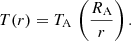
Spectral fits of similar statistical quality were obtained using two different spectral models: (1) a model with purely thermal plasma with two-temperature (2T) collisional ionization equilibrium (apec) components; the hottest plasma is at ≈30 MK; and (2) a combined thermal and nonthermal model that assumed a thermal apec component plus a power-law (see Fig. 1). In this spectral model, the thermal plasma component has a temperature of ≈10 MK. The parameters of the best-fit models are listed in Table 2.
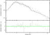 |
Fig. 1. Part of the Chandra ACIS-I spectrum of KQ Vel in the 0.5–9 keV energy range. The error bars corresponding to 3σ are shown by the data points. The solid line shows the best-fit 2T (apec) plus power-law model. The model was fit over the 0.3–11 keV energy band. The model parameters are given in Table 2. |
X-ray spectral model fitting.
When the newest calibration files that account for the contamination on the ACIS-I detector are used, the neutral hydrogen column density, NH, is consistent with being negligible in both models. Based on Fitzgerald (1970) and Ducati et al. (2001), the intrinsic color1 of an A0 star is (B − V)0 = −0.08. The observed (B − V)obs = 0.02, formally implying a negative reddening E(B − V) = (B − V)obs − (B − V)0. We interpret this as a very low level of interstellar reddening, and, correspondingly, a low neutral H column density in the direction of KQ Vel; this is consistent with the results from X-ray spectral modeling.
From the Rankine-Hugoniot condition for a strong shock, the post-shock temperature is given by T ≈ 14 MK × (vw/103 km s−1)2 for vw the wind speed. A temperature of 30 MK would require speeds exceeding 1500 km s−1. This is significantly higher than expected for A0V stars; the empirically estimated terminal wind velocities of main-sequence B-type stars, for example, do not exceed 1000 km s−1 (Prinja 1989). We favor the combined thermal and nonthermal plasma model as better motivated physically. By analogy with the Bp stars, the nonthermal X-rays in the spectrum of KQ Vel might be explained as bremsstrahlung emission from a nonthermal electron population that is also responsible for the gyro-synchrotron stellar radio emission. When they impact the stellar surface, X-rays are radiated by thick-target bremsstrahlung emission. This physical process is well understood; in particular, the spectral index α of the nonthermal photons can be related to the spectral index δ of the nonthermal electron population by the simple relation δ = α + 1 (Brown 1971). When the best-fit X-ray spectrum of KQ Vel is used, the spectral index of the nonthermal electron energy distribution then is δ = 3.5.
The X-ray light curve of KQ Vel shown in Fig. 2 is variable. The power-density spectrum was calculated using a Fourier algorithm (Horne & Baliunas 1986).
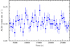 |
Fig. 2. X-ray light curve of KQ Vel. Data are for the 0.3–10.0 keV (1.24–62 Å) energy band, where the background was subtracted. The horizontal axis denotes the time after the beginning of the observation in seconds. The data were binned to 500 s. The vertical axis shows the count rate as measured by the ACIS-I camera. The error bars (1σ) correspond to the combination of the error in the source counts and the background counts. |
The largest peak in power density appears at the period of PX = 3125 ± 500 s, but with a false-alarm probability of 50%. Consequently, the period is not statistically significant. However, the periodicities at amplitudes that are too low to be detected with the current data cannot be ruled out.
3. Discussion
The Chandra data reveal that KQ Vel is extraordinary in its X-ray properties. Not only is this star one of the most luminous, it is also the hardest X-ray source of the Ap-type stars. In the following sections, we explore several different models in an attempt to explain the observed X-ray properties of KQ Vel: the overall level of X-ray emission, and its hardness and variability.
3.1. Auroral X-ray emission of a magnetic Ap star
Recent improvements in the MCWS models account for the auroral emission, and are capable of explaining jointly radio and X-ray observations of magnetic B2Vp stars (Leto et al. 2017, 2020). The auroral model was also successfully applied to the Ap star CU Vir (Robrade et al. 2018). However, there are principal differences between CU Vir and KQ Vel. The former is a fast rotator (Prot ≈ 0.52 d), whereas the latter rotates very slowly (Prot ≈ 2800 d). Furthermore, the polar field of CU Vir is about twice smaller than for KQ Vel (Kochukhov et al. 2014). A high field strength is a key parameter when plasma electrons or protons are to be accelerated to relativistic energies. Upon impinging on the stellar surface at the polar caps, this population of nonthermal particles (electrons/protons) radiates nonthermal X-rays by thick-target bremsstrahlung. The viewing geometry of KQ Vel is favorable for always showing the same stellar magnetic pole (Bailey et al. 2015). On the other hand, stellar rotation has a key role in the generation of the nonthermal electrons. In slow rotators, such as KQ Vel, the centrifugal effect that helps the trapped material to break the magnetic field lines becomes negligible. Therefore the density of the thermal electrons at the equatorial current sheet is far lower than for fast rotation. All ApBp stars with detected auroral radio or/and X-ray emission are fast rotators. In the case of the B2V star ρ Oph A, whose X-ray emission is mainly sustained by auroral mechanism, the ratio of the X-ray and radio luminosity is LX/Lν, radio = 1014 Hz (Leto et al. 2020). When this ratio is adopted, the expected radio luminosity of KQ Vel is at the mJy level.
We believe that the auroral mechanism can be responsible for the nonthermal spectral component in the X-ray spectrum of KQ Vel. However, additional mechanisms must be invoked to explain its thermal X-ray emission.
3.2. Binarity with a nondegenerate companion
KQ Vel is a binary star. The analysis of radial velocity variations by Bailey et al. (2015) suggests a companion of around 2 M⊙. The authors argued that such a companion could not be an optical star because spectral features betraying its nature would have been detected. They concluded that the companion is a compact object, either a neutron star (NS) or a black hole (BH). In addition, they considered that a hierarchical system might be a possibility, perhaps with two lower mass companions in a tighter binary.
In this latter scenario, the unusually hard and luminous X-rays might be coronal in nature, arising from either one or both of the companions. However, the KQ Vel X-ray luminosity is 3–5 times greater than that of the stars II Peg (Testa et al. 2004) or σ Gem (Huenemoerder et al. 2013), which are considered strong coronal sources (D. Huenemoerder, priv. comm.).
The companion might be an active RS CVn-type binary consisting of coronal stars. These binaries have typical X-ray luminosities of 1030 − 1031 erg s−1 (Walter & Bowyer 1981; Dempsey et al. 1993), that is, similar to the luminosity observed in KQ Vel. Montes et al. (1995) studied the behavior of activity indicators, such as Hα, Ca II K, and X-ray emission in a sample of 51 chromospherically active binary systems. It was demonstrated that the activity indicators are correlated. If X-ray luminosity of KQ Vel were due to a hidden RS CVn-type companion, we would expect that its contribution to Hα, Hϵ, and Ca II K lines would be observed in the KQ Vel spectra. However, Bailey et al. (2015) did not report peculiarities in these lines, especially in Ca II K (see their Sect. 6.5). We therefore discard a RS CVn companion as a possible explanation for the X-ray emission from KQ Vel for now.
Han et al. (2003) performed a binary population synthesis that predicted a large population of A0+sdB binary stars. The typical mass of an sdOB star is lower than the companion mass in KQ Vel, moreover, the X-ray luminosity of KQ Vel is significantly higher than that of sdOB stars (Mereghetti & La Palombara 2016). At present, we consider this scenario unlikely.
3.3. Binary with a degenerate companion
Bailey et al. (2015) proposed that KQ Vel has an NS or a BH companion. An immediate question is whether this might explain the remarkable X-ray emission of KQ Vel.
3.3.1. Accreting neutron star, medium-age pulsar, or cataclysmic variable?
The wind mass-loss rate from an A0 star is very low (Babel 1996). An upper limit of 10−12 M⊙ yr−1 has been determined for CU Vir (Krtička et al. 2019), which has the same spectral type as KQ Vel. Based on spindown considerations and if Eq. (25) from Ud-Doula et al. (2009) were used, KQ Vel would achieve its slow rotation after ∼200 Myr at a mass-loss rate of 10−13 M⊙ yr−1, while it would take ∼2 Gyr at 10−15 M⊙ yr−1. Kochukhov & Bagnulo (2006) estimated that the age of KQ Vel is 260 Myr (assuming a single-star evolution). If the secondary that we observe now as KQ Vel was re-rejuvenated due to binary mass exchange or merger, it may be even younger. We therefore roughly assume Ṁ ∼ 10−13 M⊙ yr−1 as consistent with both the stellar age and spectral type of KQ Vel.
Adopting this in calculations of the accretion rate onot a NS (Davidson & Ostriker 1973), the resulting X-ray luminosity of KQ Vel would be ∼1027 erg s−1, which is a few orders of magnitude below the observed luminosity. Furthermore, the strong magnetic field of KQ Vel dominates its feeble stellar wind. As a result, the plasma-β is very low (Altschuler & Newkirk 1969). Using Eq. (5) from Oskinova et al. (2011) and adopting as an upper limit on the wind speed of 1000 km s−1, we roughly estimate the Alfvén radius of KQ Vel as > 150 R*, which is well within the orbital separation of 245 R*. This means that only a small fraction of the wind (≲1%) that consists of neutral hydrogen and metals can escape the stellar magnetosphere and feed the NS. Hence, we can rule out direct accretion onto a compact object as an explanation for the observed X-ray luminosity.
Medium-age rotation-powered pulsars can emit X-rays at the level we observe in KQ Vel (Becker & Truemper 1997; Kargaltsev et al. 2005). In this case, the pulsed X-ray emission modulated with an NS spin period of less than a dozen seconds is expected. Unfortunately, our Chandra data are poorly suited to search for such pulsation. The X-ray spectra of KQ Vel are consistent with the presence of thermal optically thin plasma. This is quite different from the X-ray spectra of rotation-powered pulsars. The current data therefore probably do not support the presence of a middle-age pulsar in the KQ Vel system.
Some commonly detected Galactic X-ray sources are cataclysmic variables (CV; e.g., Revnivtsev et al. 2006). These interacting binaries consist of an accreting white dwarf (WD) and a low-mass donor star filling its Roche lobe. The X-ray luminosities and hard X-ray spectra of CVs might be comparable with those observed in KQ Vel. Many CVs have relatively weak and broad emission lines in their spectra. Combined with greater faintness of CVs compared to A stars, this might lead to an undetectable Ap+CV triple system2.
This meets difficulties, however, given the vast difference in ages among A-type stars and typical CVs. The age of the optical star in KQ Vel is < 300 Myr. At this age, a WD may already be formed, but generally, CVs belong to much older stellar populations. The Ap star in the KQ Vel system might be the result of a merger and might therefore be rejuvenated (see Sect. 3.4). Nevertheless, even in this case, it would require fine tuning to produce an AOV+CV system. Another consideration against a CV nature of the KQ Vel companion is that some CVs are associated with novae. For such a bright (V = 6.11 mag) and nearby star, a historical nova would have a good chance to be noticed if it occurred at the time of existing southern hemisphere records. However, because the typical recurrence time for classical novae is some hundreds of years, a nova outburst associated with KQ Vel might have been missed. While we currently do not favor the CV nature of the KQ Vel companion, this explanation can therefore not be ruled out.
3.3.2. Propelling neutron star
When a magnetized NS is embedded in a stellar wind with a very low mass-loss rate, such as in KQ Vel, the quasi-spherical subsonic regime of accretion sets in (Shakura et al. 2012). The wind is gravitationally captured from a volume much larger than determined by the outer boundary of the corotating portion of the NS magnetosphere, RA. We denote the characteristic radius of the volume from which material can be captured RB. In a rotating NS, the Keplerian radius is defined as RK = (GMNS/ω2)1/3 with ω = 2π/PNS for the NS spin period. If the condition RK ≤ RA is met, the accretion is throttled through the “propeller effect” (Illarionov & Sunyaev 1975). When the captured gas lacks the specific angular momentum to pass into the corotating magnetosphere, the accumulated wind material can form an extended, quasi-spherical envelope of hot, X-ray emitting gas.
In this situation, the NS is not accreting, and the captured stellar wind remains in the NS gravitational potential. The energy source preventing the gas from cooling is the mechanical power supplied by a propelling NS, which is mediated by the magnetic forces and convection in the shell. In this sense, the mass-loss from the optical star is not the parameter that directly regulates the shell structure. The stellar wind velocity is much more important (see the Appendix); it determines the outer shell radius. The density at the shell base, ρA, is related to the total mass of the gas in the shell that determines the observed emission measure (EM; using a crude analogy, the gas density near the ground on Earth is determined by the total mass and temperature of the terrestrial atmosphere). ρA is therefore not directly related to the poorly known stellar wind mass-loss rate. X-ray emission from the gas shell is sustained by the NS spin-down and not by wind accretion, therefore the orbital eccentricity is not relevant.
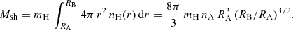
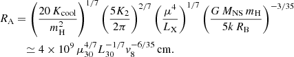
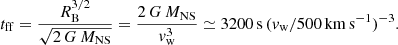
It is possible to obtain a self-consistent solution for the hot envelope using the parameters of KQ Vel. The detailed model calculations are described in the Appendix. We adopted an NS mass of MNS = 1.5 M⊙ and used constraints from the X-ray observations: LX ≈ 2 × 1030 erg s−1, EM ≈ 5 × 1052 cm−3, and  keV (Table 2). Following the theory of quasi-spherical accretion, the derived inner and outer radii (RA and RB), the mass of the shell Msh, the wind speed of the A0p star, and the magnetic moment (μ) of the NS are then vw ≈ 500 km s−1, RA ≈ 0.1 R⊙, RB ≈ 2.2 R⊙, μ30 ≈ 3, Msh ≈ 1 × 10⁻¹⁴ M⊙, and μ30 ≈ 3, where μ30 is the magnetic moment of the NS normalized to 1030 G cm3. This is a typical value for an NS.
The derived quantities agree well with the expected properties of the KQ Vel system. The wind speed, 500 km s−1, is appropriately realistic. The derived RA = 0.1 R⊙ implies that if the NS has spin period PNS ≲ 260 s, it will be in a propeller state. This spin period is quite reasonable for an NS that has not spun-down to the accretion stage, given the weak stellar wind of the A0p companion and a large binary separation.
While the accretion power is far too small to explain the observed X-ray luminosity of KQ Vel, the propelling NS injects significant amount of energy by interaction of the rotating magnetosphere and the matter in the shell. The maximum power that is provided by a propelling NS is 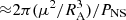 (Shakura et al. 2012). When we insert the parameters derived for KQ Vel, the NS should have PNS ≲ 100 s to explain the observed X-ray luminosity. According to Eqs. (A.15) and (A.16), the NS spin-down can power the hot shell surrounding NS in the KQ Vel system at the present level for at least 105 years.
Furthermore, the theory of quasi-spherical accretion naturally explains the variability seen in the X-ray light curve (Figs. 2). The time scale of the observed X-ray variability, PX ∼ 3000 s, is much shorter than either the orbital period of the binary (Porb = 840 d) or the spin period of the A0p star (Prot = 2800 d). At the same time, it is at least an order of magnitude longer than the predicted NS spin period, PNS ≲ 100 s. However, according to Eq. (A.13), the free-fall time of a hot convective shell surrounding the NS is tff ≃ 3200 s (vw/500 km s−1)−3, which is very similar to the observed variability timescale in KQ Vel.
Finally, we considered the special properties of KQ Vel, specifically, the strong magnetic field of the donor star and hence its magnetized wind. The estimates show (see the Appendix) that the magnetic reconnection of the accretion flow and the NS field provides an important source of plasma heating to maintain the hot envelope around the NS in the KQ Vel binary system.
3.4. Evolutionary considerations: was KQ Vel a triple?
The KQ Vel system has a wide and eccentric orbit. If an NS is present in the system, a supernova (SN) must have occurred without disrupting the binary. In the absence of an additional kick velocity, the orbital eccentricity following the SN event would become e = ΔM/(MNS + Mopt). For the parameters of KQ Vel (Table 1), ΔM = 0.36 ⋅ (3 + 1.5) = 1.6 M⊙. The NS progenitor mass can therefore be roughly estimated as 1.6 + 1.5 ≈ 3 M⊙. This likely was a He-star that was stripped during the mass-exchange event. The initial mass of the NS progenitor can then be estimated (see Postnov & Yungelson 2014) as  , or a total mass of ∼11 M⊙. When the long orbital period is taken into account, the progenitor system might have been a C-type (i.e., a wide binary). In such cases, the mass transfer can be highly unstable and likely nonconservative, and the hydrogen envelope will be lost without adding mass to the 3 M⊙ secondary companion. A sort of common envelope (CE) may have occurred, but the efficiency of CEs in wide binaries is uncertain.
A different scenario may help to shed light on the origin of KQ Vel system and its peculiar properties, particularly the strongly magnetic nature of the optical star. It has long been believed and recently confirmed by numerical modeling that magnetic stars can result from stellar mergers (Schneider et al. 2019). In this case, KQ Vel was originally a triple system, where the present-day Ap star is the merger product, possibly of a W UMa-type system. The NS is the tertiary remnant. If the initially less massive tertiary gained mass during the Roche-lobe overflow by either of the primary binary components, the orbital separation would have increased.
The eccentric Kozai-Lidov mechanism (Naoz & Fabrycky 2014) operating in triple systems causes strong inclination and eccentricity fluctuations, and leads to the tightening of the inner binary. The merger product of the inner binary is observed today as the magnetic Ap star. The tertiary, with a mass in the range 8−10 M⊙, may have evolved into an electron-capture SN without disrupting the system, and formed the NS we observe today.
The proximity of KQ Vel to Earth implies that the KQ Vel-like systems cannot be exotic and exceptionally rare. The lifetime of a propelling NS is ∼105 − 106 yr, that is, significantly shorter than the lifetime of a few ×108 yr of an A0-type star. After the NS has spun down and the propeller stage is concluded, the NS will enter the accretion regime, but given a very low accretion rate, its X-ray luminosity will be low (Sect. 3.3.1). Because of the large orbital separation, the binarity may be easily missed during a routine spectroscopic analysis. Future work on astrometric catalogs, for example, Gaia, will undoubtedly be useful to shed more light on the population of wide intermediate-mass binaries with X-ray dim NS companions.
4. Conclusions
Chandra X-ray observations of the strongly magnetic binary star KQ Vel revealed that its properties are exceptional for an Ap-type star: high X-ray luminosity, a hard spectrum, and a variable X-ray light curve. The observed spectrum can be well fit either by a multitemperature thermal plasma spectral model or by a hybrid model consisting of thermal and a nonthermal emission components. We prefer the former spectral model, and explain the nonthermal component as being due to the auroral mechanism, that is, similar to the Ap star CU Vir.
Exploring several different interpretations, we concluded that the theory of quasi-spherical accretion onto a propelling NS with PNS ≲ 100 s and μ30 ≈ 3 best describes the hot plasma temperature, its emission measure, and the timescale of X-ray variability observed in KQ Vel. Thus, new X-ray Chandra observations strongly support the suggestion of Bailey et al. (2015) of a compact companion in KQ Vel. We conclude that the compact companion is an NS in the propeller regime.
After acceptance of the paper, we received additional information from Tim Bedding. He reported that the TESS light curve of KQ Vel has a clear 2.01618 d period that is likely associated with stellar rotation. If this short rotation period were confirmed, it would imply younger age of the KQ Vel system and further support our scenario on its nature and origin.
KQ Vel is the first known strongly magnetic Ap + NS binary. Confirmation of the existence of such objects has important consequences for our understanding of binary evolution and accretion physics.
We used tables found at www.stsci.edu/~inr/intrins.html that are based on the work of the cited authors.
This possibility was suggested by the anonymous referee.
Acknowledgments
Authors are grateful to the anonymous referee for a very useful report which strongly improved the paper, and for the suggestions for future work on this interesting system. Authors thank Dr. H. Todt for sharing the statistical models. LMO acknowledges financial support by the Deutsches Zentrum für Luft und Raumfahrt (DLR) grant FKZ 50 OR 1809, and partial support by the Russian Government Program of Competitive Growth of Kazan Federal University. The work of KAP is partially supported ny RFBR grant 19-02-00790.
References
- Altschuler, M. D., & Newkirk, G. 1969, Sol. Phys., 9, 131 [Google Scholar]
- Arnaud, K. A. 1996, Astronomical Data Analysis Software and Systems V, G. H. Jacoby, & J. Barnes, ASP Conf. Ser., 101, 17 [Google Scholar]
- Asplund, M., Grevesse, N., Sauval, A. J., & Scott, P. 2009, ARA&A, 47, 481 [NASA ADS] [CrossRef] [Google Scholar]
- Babel, J. 1996, A&A, 309, 867 [Google Scholar]
- Babel, J., & Montmerle, T. 1997, A&A, 323, 121 [NASA ADS] [Google Scholar]
- Bailey, J. D., Grunhut, J., & Landstreet, J. D. 2015, A&A, 575, A115 [NASA ADS] [CrossRef] [EDP Sciences] [Google Scholar]
- Becker, W., & Truemper, J. 1997, A&A, 326, 682 [Google Scholar]
- Borra, E. F., & Landstreet, J. D. 1975, PASP, 87, 961 [NASA ADS] [CrossRef] [Google Scholar]
- Brown, J. C. 1971, Sol. Phys., 18, 489 [NASA ADS] [CrossRef] [Google Scholar]
- Cowie, L. L., McKee, C. F., & Ostriker, J. P. 1981, ApJ, 247, 908 [NASA ADS] [CrossRef] [Google Scholar]
- Davidson, K., & Ostriker, J. P. 1973, ApJ, 179, 585 [NASA ADS] [CrossRef] [Google Scholar]
- Dempsey, R. C., Linsky, J. L., Fleming, T. A., & Schmitt, J. H. M. M. 1993, ApJS, 86, 599 [NASA ADS] [CrossRef] [Google Scholar]
- Ducati, J. R., Bevilacqua, C. M., Rembold, S. R. B., & Ribeiro, D. 2001, ApJ, 558, 309 [Google Scholar]
- Fitzgerald, M. P. 1970, A&A, 4, 234 [NASA ADS] [Google Scholar]
- Han, Z., Podsiadlowski, P., Maxted, P. F. L., & Marsh, T. R. 2003, MNRAS, 341, 669 [NASA ADS] [CrossRef] [Google Scholar]
- Horne, J. H., & Baliunas, S. L. 1986, ApJ, 302, 757 [Google Scholar]
- Huenemoerder, D. P., Phillips, K. J. H., Sylwester, J., & Sylwester, B. 2013, ApJ, 768, 135 [CrossRef] [Google Scholar]
- Illarionov, A. F., & Sunyaev, R. A. 1975, A&A, 39, 185 [NASA ADS] [Google Scholar]
- Jaschek, M., & Jaschek, C. 1959, PASP, 71, 48 [NASA ADS] [CrossRef] [Google Scholar]
- Kargaltsev, O. Y., Pavlov, G. G., Zavlin, V. E., & Romani, R. W. 2005, ApJ, 625, 307 [NASA ADS] [CrossRef] [Google Scholar]
- Kochukhov, O., & Bagnulo, S. 2006, A&A, 450, 763 [NASA ADS] [CrossRef] [EDP Sciences] [Google Scholar]
- Kochukhov, O., Lüftinger, T., Neiner, C., Alecian, E., & MiMeS Collaboration 2014, A&A, 565, A83 [NASA ADS] [CrossRef] [EDP Sciences] [Google Scholar]
- Krtička, J., Mikulášek, Z., Henry, G. W., et al. 2019, A&A, 625, A34 [CrossRef] [EDP Sciences] [Google Scholar]
- Leto, P., Trigilio, C., Oskinova, L., et al. 2017, MNRAS, 467, 2820 [NASA ADS] [CrossRef] [Google Scholar]
- Leto, P., Trigilio, C., Oskinova, L. M., et al. 2018, MNRAS, 476, 562 [NASA ADS] [CrossRef] [Google Scholar]
- Leto, P., Trigilio, C., Leone, F., et al. 2020, MNRAS, 493, 4657 [CrossRef] [Google Scholar]
- Mathys, G. 2017, A&A, 601, A14 [NASA ADS] [CrossRef] [EDP Sciences] [Google Scholar]
- Mereghetti, S., & La Palombara, N. 2016, Adv. Space Res., 58, 809 [NASA ADS] [CrossRef] [Google Scholar]
- Montes, D., Fernandez-Figueroa, M. J., de Castro, E., & Cornide, M. 1995, A&A, 294, 165 [NASA ADS] [Google Scholar]
- Naoz, S., & Fabrycky, D. C. 2014, ApJ, 793, 137 [NASA ADS] [CrossRef] [Google Scholar]
- Oskinova, L. M., Todt, H., Ignace, R., et al. 2011, MNRAS, 416, 1456 [NASA ADS] [CrossRef] [Google Scholar]
- Postnov, K. A., & Yungelson, L. R. 2014, Liv. Rev. Rel., 17, 3 [NASA ADS] [CrossRef] [PubMed] [Google Scholar]
- Postnov, K., Oskinova, L., & Torrejón, J. M. 2017, MNRAS, 465, L119 [Google Scholar]
- Prinja, R. K. 1989, MNRAS, 241, 721 [NASA ADS] [CrossRef] [Google Scholar]
- Raymond, J. C., Cox, D. P., & Smith, B. W. 1976, ApJ, 204, 290 [NASA ADS] [CrossRef] [Google Scholar]
- Revnivtsev, M., Sazonov, S., Gilfanov, M., Churazov, E., & Sunyaev, R. 2006, A&A, 452, 169 [NASA ADS] [CrossRef] [EDP Sciences] [Google Scholar]
- Robrade, J. 2016, Adv. Space Res., 58, 727 [NASA ADS] [CrossRef] [Google Scholar]
- Robrade, J., Oskinova, L. M., Schmitt, J. H. M. M., Leto, P., & Trigilio, C. 2018, A&A, 619, A33 [NASA ADS] [CrossRef] [EDP Sciences] [Google Scholar]
- Schneider, F. R. N., Ohlmann, S. T., Podsiadlowski, P., et al. 2019, Nature, 574, 211 [NASA ADS] [CrossRef] [Google Scholar]
- Schröder, C., & Schmitt, J. H. M. M. 2007, A&A, 475, 677 [NASA ADS] [CrossRef] [EDP Sciences] [Google Scholar]
- Shakura, N., Postnov, K., Kochetkova, A., & Hjalmarsdotter, L. 2012, MNRAS, 420, 216 [NASA ADS] [CrossRef] [Google Scholar]
- Syunyaev, R. A., & Shakura, N. I. 1977, Sov. Astron. Lett., 3, 138 [NASA ADS] [Google Scholar]
- Testa, P., Drake, J. J., Peres, G., & DeLuca, E. E. 2004, ApJ, 609, L79 [NASA ADS] [CrossRef] [Google Scholar]
- Ud-Doula, A., Owocki, S. P., & Townsend, R. H. D. 2009, MNRAS, 392, 1022 [NASA ADS] [CrossRef] [Google Scholar]
- Walter, F. M., & Bowyer, S. 1981, ApJ, 245, 671 [NASA ADS] [CrossRef] [Google Scholar]
Appendix A: X-ray emission from a hot shell around a propelling neutron star in a settling accretion regime
The X-ray emission properties from a hot shell around the magnetosphere of a propelling neutron star (a model applied to the γ Cas phenomenon) were calculated in Postnov et al. (2017; see Eqs. (2)–(11) in that paper). The calculations were carried out for the case of thermal bremsstrahlung cooling, which is valid for high plasma temperatures kT ≳ 4 keV. At lower plasma temperatures, the collisional cooling function becomes dominant, rapidly increasing down to temperatures ∼0.01 keV. To estimate the properties of the shell in the temperature range 0.01 < kT < 4 keV, we can use the analytical approximation for a fully ionized plasma with solar abundances (Raymond et al. 1976; Cowie et al. 1981),
 (A.1)
(A.1)
with Kcool = 6.2 × 10⁻¹⁹ in cgs units. Below we replace the numerical power 0.6 with 3/5.
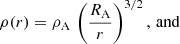
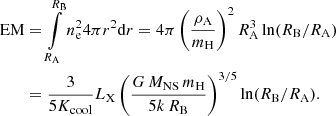
The total X-ray luminosity from an optically thin spherical shell located between the magnetospheric radius RA and the outer radius RB is
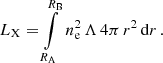 (A.2)
(A.2)
Here we assumed a completely ionized H gas, with nH = ne = ρ/mH. For the outer boundary in the integral (A.2), we assumed a Bondi radius with 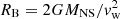 , where MNS is the NS mass and vw is the velocity of the wind from the optical star, and we neglected the orbital motion of the NS.
The density and temperature profiles in quasi-stationary gas envelope surrounding the NS magnetosphere (Shakura et al. 2012) are
 (A.3)
(A.3)
 (A.4)
(A.4)
Using the virial temperature of a monoatomic gas at the base of the shell TA = GMNSmH/5kRA, we obtain
![Mathematical equation: $$ \begin{aligned} L_{\rm X}=4\pi \frac{5}{3}K_\mathrm{cool} \left(\frac{ \rho _{\rm A}}{m_{\rm H}} \right)^2R_{\rm A}^3\left(\frac{GM_{\rm NS} m_{\rm H}}{5kR_{\rm B}} \right)^{-3/5}\left[1-\left(\frac{R_{\rm A}}{R_{\rm B}}\right)^{3/5}\right]. \end{aligned} $$](/articles/aa/full_html/2020/09/aa38214-20/aa38214-20-eq10.gif) (A.5)
(A.5)
An important difference of Eq. (A.5) from the analogous Eq. (6) in Postnov et al. (2017) is that due to the inverse power-law temperature dependence of Λ, the X-ray luminosity is almost fully determined by the combination  and the stellar wind velocity vw (which sets the Bondi radius by
 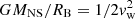 ). The ratio RA/RB is typically ≪1, which enables us to omit the second term in the square brackets in Eq. (A.5). The EM in the shell becomes
 (A.6)
(A.6)
Noting that 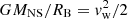 and substituting the characteristic values MNS = 1.5 M⊙, vw = 108 cm s−1 × v8, LX = 1030 erg s−1 × L30, we arrive at
 (A.7)
(A.7)
The logarithmic factor here is usually on the order of 3–4. The EM is observationally constrained, therefore it is possible to determine the mass contained in the shell with
 (A.8)
(A.8)
Using Eq. (A.5) and the density and temperature profiles in the shell, we can derive the expression for the magnetospheric radius RA in a straigthforward way,
 (A.9)
(A.9)
Here μ = 1030 G cm3 μ30 is the NS magnetic moment, K2 ≈ 7.7 is a numerical factor that takes the difference of the NS magnetosphere from a pure dipole shape into account (cf., Shakura et al. 2012). For typical wind velocities, 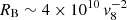 cm, and therefore our assumption RB/RA ≫ 1 is justified.
The temperature at the base of the shell is  . However, neither the maximum nor the minimum temperature is relevant to the fit of the observed spectrum, but the average temperature as weighted by the EM. The predicted average temperature,
  , is given by
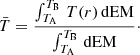 (A.10)
With dEM = n2(r) 4π r2 dr, and with the preceding expressions, along with RB ≫ RA, the weighted average temperature becomes
 (A.11)
Because the denominator is typically on the order of a few, the characteristic thermal temperature expected from the hot-shell model is a factor of a few lower than the temperature at the inner boundary of the shell.
The column density distribution of material in the shell is related to the spectral fitting. Even if hydrogen is completely ionized in the hot shell, it is standard to express the column as NH. Much of the absorption at the higher energies derives from photoabsorption by metals. Along a radial through the annual shell and assuming RB/RA ≫ 1, the column density is
 (A.12)
Equations (A.5), (A.6), (A.11) enable us to express three independent model parameters, ρA, RA, and RB (or vw) through the values that are directly derived from observations: LX, EM, and  . Then, Eq. (A.9) can be used to estimate the NS magnetic field.
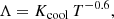
Finally, we determined whether the shell can remain hot in the assumed form of the cooling function that increases along the radius as Λ ∼ T−0.6 ∼ r0.6. The free-fall time of the hot envelope is given by
 (A.13)
The plasma cooling time in the isentropic shell can be expressed as
![Mathematical equation: $$ \begin{aligned} t_{\rm cool}(r)&=\frac{3kT}{n_{\rm e}\Lambda }\simeq 10^3\, [\mathrm{s} ]\frac{T_{\rm A}^{8/5}(R_{\rm A}/r)^{8/5}}{n_{\rm a}(R_{\rm A}/r)^{3/2}} \nonumber \\&=10^3\,[\mathrm{s} ]\left(\frac{R_{\rm A}}{r}\right)^{1/10} \left[\frac{\ln (R_{\rm B}/R_{\rm A})}{3}\right]^{1/2} \left(\frac{\mathrm{EM} }{5\times 10^{52}\,\mathrm{cm} ^{-3}}\right)^{-1/2} , \end{aligned} $$](/articles/aa/full_html/2020/09/aa38214-20/aa38214-20-eq26.gif) (A.14)
(A.14)
which is almost constant across the shell. However, this time is dangerously close to the free-fall time tff ∼ 3 × 10³[s](r/RB)3/2. This suggests that if there were no additional plasma heating in the shell, the captured gas would rapidly cool below RB to form a cold dense “dead” disk around the magnetosphere (Syunyaev & Shakura 1977), and no hot convective shell would be formed.
In the case of magnetized wind, the magnetic reconnection can heat the plasma. The reconnection time in a magnetized plasma blob of size l, mass mb ∼ ρbl3, and magnetic field Bb can be written as tr ∼ l/vr, where vr is the reconnection rate, which scales as the Alfvén velocity  . Therefore,
  , and using the magnetic flux conservation
  , we arrive at
 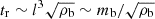 . The magnetic reconnection heating is effective if
  . By neglecting the mass decrease of the falling blob (due to, e.g., Kelvin-Helmholtz stripping) and assuming that the adiabatic blob evolves (i.e., ρbTbl5/3 = const) in the surrounding plasma with pressure Pe ∼ neTe and pressure balance Pb ∼ ρbTb = Pe, we arrive at
  (here the adiabatic scaling for the surrounding plasma density and temperature, Eqs. (A.3) and (A.4), were applied). This means that the magnetic reconnection in freely falling magnetized plasma blobs can rapidly occur and provide additional heat that sustains the hot convective shell. In addition to the plasma heating, the magnetic blob reconnection results in the generation of a ∼10% nonthermal tail. Realistically, not all free-falling blobs are magnetized, and part of them can cool down and thus increase NH relative to the hot plasma estimate Eq. (A.12) above.
The spin-down timescale of the propelling NS is
 (A.15)
where I is the NS moment of inertia, and ϵ = Lmr/Lsd is the ratio of the NS spin-down power,  , to the power supplied by magnetic reconnection. Then
![Mathematical equation: $$ \begin{aligned} t_{\rm sd}\simeq 2\times 10^5\,[\mathrm{yr} ] \left(\frac{P_{\rm NS}}{100\,\mathrm{s} }\right)^{-2} \left(\frac{L_{\rm X}}{10^{30}\,\mathrm {erg\,s} ^{-1}}\right)(1+\epsilon ). \end{aligned} $$](/articles/aa/full_html/2020/09/aa38214-20/aa38214-20-eq35.gif) (A.16)
(A.16)
All Tables
All Figures
|
Fig. 1. Part of the Chandra ACIS-I spectrum of KQ Vel in the 0.5–9 keV energy range. The error bars corresponding to 3σ are shown by the data points. The solid line shows the best-fit 2T (apec) plus power-law model. The model was fit over the 0.3–11 keV energy band. The model parameters are given in Table 2. |
| In the text | |
|
Fig. 2. X-ray light curve of KQ Vel. Data are for the 0.3–10.0 keV (1.24–62 Å) energy band, where the background was subtracted. The horizontal axis denotes the time after the beginning of the observation in seconds. The data were binned to 500 s. The vertical axis shows the count rate as measured by the ACIS-I camera. The error bars (1σ) correspond to the combination of the error in the source counts and the background counts. |
| In the text | |
Current usage metrics show cumulative count of Article Views (full-text article views including HTML views, PDF and ePub downloads, according to the available data) and Abstracts Views on Vision4Press platform.
Data correspond to usage on the plateform after 2015. The current usage metrics is available 48-96 hours after online publication and is updated daily on week days.
Initial download of the metrics may take a while.