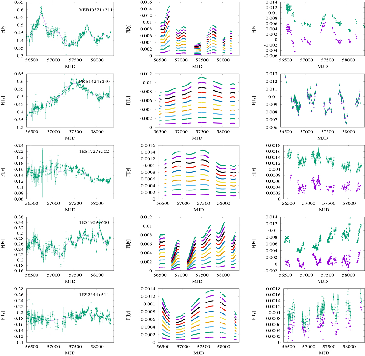
Steps of the analysis used to determine the contribution of the common emission component at radio and optical frequencies. Left: fitting a polynomial to the radio light curve. Middle: polynomial fit scaled to the average flux of the optical light curve and multiplied with a scaling factor (different colours correspond to different scaling factors, see text). Right: scaled polynomial is subtracted from the optical data (green filled circles with errors). The RMS of the resulting light curve (purple filled circles) is compared with the RMS of the original data. These analysis steps are shown for all sources from bottom to top: VER J0521+211, PKS 1424+240, 1ES 1727+502, 1ES 1959+650 and 1ES 2344+514. In the case of PKS 1424+240 subtracting the polynomial did not decrease the RMS of the optical light curve and therefore the purple dots are under the green symbols and are not well visible in the rightmost panel.