| Issue |
A&A
Volume 640, August 2020
|
|
|---|---|---|
| Article Number | A47 | |
| Number of page(s) | 15 | |
| Section | Cosmology (including clusters of galaxies) | |
| DOI | https://doi.org/10.1051/0004-6361/202037683 | |
| Published online | 10 August 2020 | |
Correlation function: biasing and fractal properties of the cosmic web
1
Tartu Observatory, University of Tartu, 61602 Tõravere, Estonia
e-mail: This email address is being protected from spambots. You need JavaScript enabled to view it.
2
Estonian Academy of Sciences, 10130 Tallinn, Estonia
3
ICRANet, Piazza della Repubblica, 10, 65122 Pescara, Italy
4
National Institute of Chemical Physics and Biophysics, Tallinn 10143, Estonia
Received:
7
February
2020
Accepted:
8
June
2020
Abstract
Aims. Our goal is to determine how the spatial correlation function of galaxies describes biasing and fractal properties of the cosmic web.
Methods. We calculated spatial correlation functions of galaxies, ξ(r), structure functions, g(r) = 1 + ξ(r), gradient functions, γ(r) = d log g(r)/d log r, and fractal dimension functions, D(r) = 3 + γ(r), using dark matter particles of the biased Λ cold dark matter (CDM) simulation, observed galaxies of the Sloan Digital Sky Survey (SDSS), and simulated galaxies of the Millennium and EAGLE simulations. We analysed how these functions describe fractal and biasing properties of the cosmic web.
Results. The correlation functions of the biased ΛCDM model samples at small distances (particle and galaxy separations), r ≤ 2.25 h−1 Mpc, describe the distribution of matter inside dark matter halos. In real and simulated galaxy samples, only the brightest galaxies in clusters are visible, and the transition from clusters to filaments occurs at a distance r ≈ 0.8−1.5 h−1 Mpc. At larger separations, the correlation functions describe the distribution of matter and galaxies in the whole cosmic web. The effective fractal dimension of the cosmic web is a continuous function of the distance (separation). Real and simulated galaxies of low luminosity, Mr ≥ −19, have almost identical correlation lengths and amplitudes, indicating that dwarf galaxies are satellites of brighter galaxies, and do not form a smooth population in voids.
Conclusions. The combination of several physical processes (e.g. the formation of halos along the caustics of particle trajectories and the phase synchronisation of density perturbations on various scales) transforms the initial random density field to the current highly non-random density field. Galaxy formation is suppressed in voids, which increases the amplitudes of correlation functions and power spectra of galaxies, and increases the large-scale bias parameter. The combined evidence leads to the large-scale bias parameter of L⋆ galaxies the value b⋆ = 1.85 ± 0.15. We find r0(L⋆) = 7.20 ± 0.19 for the correlation length of L⋆ galaxies.
Key words: large-scale structure of Universe / dark matter / cosmology: theory / galaxies: halos / methods: numerical
© ESO 2020
1. Introduction
Early data on the distribution of galaxies came from the counts of galaxies on the sky. The available data suggested that the distribution of galaxies on the sky is dominated by an almost random field population with randomly spaced clusters. The distribution can be described by the two-point correlation function of galaxies (Peebles 1980). The two-point correlation is a function of distance and describes the excess probability of finding two galaxies separated by this distance. It is not sensitive to the pattern of the cosmic web because it measures only the amplitude of the density fluctuations of the density field of galaxies, not the phase information, which is essential to describe the cosmic web. To investigate the structure of the cosmic web in detail, various other methods have been developed. For a recent overview, see van de Weygaert et al. (2016). In spite of these limitations, large areas in the study of galaxy distribution exist where the two-point correlation function and its Fourier companion, the power spectrum of density perturbations, are useful.
One area in which the correlation functions can be applied is the biasing phenomenon. Peebles & Groth (1975) showed that the two-point correlation function of galaxies can be represented as a power law ξ(r) = (r/r0)γ, where r0 ≈ 5 h−1 Mpc is the correlation length, and γ ≈ −1.7 is the slope of the correlation function. The bias parameter b can be defined as the ratio of the amplitudes of the galaxy correlation functions (or power spectra P) to the mass, b2 = Pg/Pm. The analyses of galaxy correlation functions by Lahav et al. (2002), Verde et al. (2002), and Zehavi et al. (2005) suggested that the large-scale bias parameter is b ≈ 1. A similar result was found from the analysis of power spectra of galaxies by Tegmark et al. (2004a) and Zehavi et al. (2011).
In contrast, Einasto et al. (1993, 1999) showed that the bias parameter is inversely proportional to the fraction of matter in galaxies, b = 1/Fg, which means that b > 1. Mandelbaum et al. (2013) used luminous red giant (LRG) galaxies of the Sloan Digital Sky Survey (SDSS) to obtain a value of b ≈ 2 for the large-scale bias. Klypin et al. (2016) used several MultiDark simulations and determined the bias factor of power spectra of halos to the power spectra of mass, b = 1.95. Einasto et al. (2019) compared power spectra of biased samples of a Λ cold dark matter (CDM) model with the full dark matter (DM) sample of the same model. The authors found the value b* = 1.85 ± 0.15 for the bias parameter of the model equivalent of L* galaxies.
The reason for this large difference in bias parameter estimates was not clear. In order to understand what causes the differences between various determinations of bias parameters, we need to analyse the technique of the correlation function analysis in more detail.
The main goal of this paper is to understand the biasing phenomenon as the relation between distributions of matter and galaxies by applying the two-point correlation function. In doing so, we determine why analyses of correlation functions and power spectra of galaxies yield very different values for the bias parameter b.
The slope of the correlation function γ contains information on the fractal character of the cosmic web. Early data suggested that a power law with fixed γ is valid over a very wide range of distances. It is currently well accepted that galaxies form in DM-dominated halos (White & Rees 1978). Thus the spatial correlation function at small separations r characterises the galaxy distribution within DM-dominated halos or clusters, and on larger separations, the galaxy distribution in the whole cosmic web. This leads to departures of the correlation function from a pure power law. The study of fractal properties of the cosmic web using correlation functions of various samples is the second goal of this paper. The relation between spatial and projected correlation functions is investigated in a separate paper by Einasto et al. (2020).
Following Einasto et al. (2019), we use a ΛCDM model as basis that is calculated in a box of size 512 h−1 Mpc. In the simulations we select particles from the same set for biased samples and for unbiased samples, and observational selection effects can be ignored. We take advantage of the fact that the positions of all particles are known for this model. This allows us to compare correlation functions of dark matter and simulated galaxies differentially.
For the comparison, we analyse absolute magnitude (volume) limited SDSS samples, as found by Liivamägi et al. (2012) and Tempel et al. (2014a). We also analyse the galaxy samples from the Millennium simulation by Springel et al. (2005) and the galaxy catalogues of the EAGLE simulation provided by McAlpine et al. (2016).
To investigate biasing and fractal properties of the cosmic web in more detail, we use the galaxy correlation function, ξ(r), and its derivatives: the structure function, g(r) = 1 + ξ(r), its log-log gradient, the gradient function, γ(r) = d log g(r)/d log r, and the fractal dimension function, D(r) = 3 + γ(r) = 3 + dlog g(r)/d log r.
The paper is organised as follows. In the next section we describe the simulation and the observational data we used, the methods for calculating the correlation functions and their derivatives, and the first results of the analysis of these functions for simulated and real galaxy samples of various luminosity limits. In Sect. 3 we discuss the biasing properties of LCDM and galaxy samples, and the luminosity dependence of the correlation functions and their derivatives. In Sect. 4 we study the fractal properties of the cosmic web as described by the correlation function and its derivatives. The last section presents our conclusions.
2. Methods, data, and first results
In this section we describe the simulation and the observational data we used and the methods for calculating the correlation functions. We start by describing the methods for calculating the correlation and related functions. Thereafter we describe the ΛCDM numerical simulation we used to determine density fields at various density threshold levels to simulate galaxy samples of different luminosity. Next we describe our basic observation sample selected from the Sloan Digital Sky Survey (SDSS) and from the EAGLE and Millennium simulations, which we used for comparison with observational samples. Finally, we describe our first results from calculating the correlation functions.
2.1. Calculation of the correlation functions
The natural estimator to determine the two-point spatial correlation function is
 (1)
(1)
and the Landy & Szalay (1993) estimator is
 (2)
(2)
In these formulae, r is the galaxy pair separation (distance), and DD(r), DR(r), and RR(r) are normalised counts of galaxy-galaxy, galaxy-random, and random-random pairs at a distance r of the pair members.
We applied the Landy & Szalay (1993) estimator for the samples of SDSS galaxies, and the natural estimator for the cubical EAGLE and Millennium model galaxy samples. The model samples have two scale parameters, the length of the cube, L in h−1 Mpc, and the maximum distance for calculating the correlation function, Lmax. The second parameter is used to exclude pairs with separations larger than Lmax in the loop over galaxies to count pairs. This speeds up the calculations considerably. The separation interval r from 0 to Lmax was divided into 100 equal bins of length Lmax/100 in case of the EAGLE and Millennium samples, and into Nb equal bins of length log Lmax/Nb for the SDSS samples. By varying Lmax and Nb, we can use different bin sizes that are optimised for the particular sample. The core of the Fortran program we used for the Millennium and EAGLE samples was written previously to investigate galaxy correlation functions by Einasto et al. (1997a,b, 1986) and Klypin et al. (1989). At these times, computers were very slow and optimisation of programs was crucial. The random-random pair count RR(r) was found by applying the random number generator ran2 by Press et al. (1992), using one or two million particles. To speed up the calculation of random-random pairs, we split random samples into ten independent subsamples, as was also done by Keihänen et al. (2019).
The ΛCDM model samples contain all particles with local density labels ρ ≥ ρ0. To derive correlation functions of these samples, a conventional method cannot by used because the number of particles is too large, up to 5123 in the full unbiased model. To determine the correlation functions of the ΛCDM samples, we used the Szapudi et al. (2005) method. Conventional methods scale as O(N2). When the number of objects N becomes large, the method is too slow. Measurements of power spectra can be obtained with fast Fourier transforms (FFT), which scale as O(N log N). The Szapudi et al. (2005) method also uses the FFT to calculate correlation functions and scales as O(N log N). The method is an implementation of the algorithm eSpICE, the Euclidean version of SpICE by Szapudi et al. (2001). As input, the method uses density fields on grids 10243, 20483, and 30723. Correlation functions are found with Lmax = 100 h−1 Mpc, and with 200, 400, and 600 linear bins, respectively.
In the following analysis we use the spatial correlation function, ξ(r), and the pair correlation or structure function, g(r) = 1 + ξ(r), to characterise the galaxy distribution in space; for details see Martínez & Saar (2002). Instead of the slope of the correlation function as a parameter, γ, we calculate the log-log gradient of the pair correlation function as a function of distance,
 (3)
(3)
which we call gradient function, or simply γ(r) function. It is related to the effective fractal dimension D(r) of samples at mean separation of galaxies at r,
 (4)
(4)
We call the D(r) = 3 + γ(r) function the fractal dimension function. Martínez & Saar (2002) defined the correlation dimension  , where
  is the average of the structure function,
 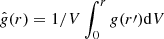 . For our study we prefer to use the local value of the structure function to define its gradient. The effective fractal dimension of a random distribution of galaxies is D = 3, and γ = 0, respectively; in sheets, D = 2 and γ = −1; in a filamentary distribution, D = 1 and γ = −2; and within clusters, D = 0 and γ = −3.
To determine the gradient function γ(r), we use a linear fit of the structure function g(r). At small distances, the function changes very rapidly, and we use for its gradient at r just the previous and following log g(r) value divided by the log step size in r. At larger distances, we use a linear fit on the distance interval in ±m steps from the particular r value of log g(r), presented as a table. The fit is computed using the fit subroutine by Press et al. (1992), which gives the gradient and its error. The correlation functions and their derivatives were calculated with a constant linear or logarithmic step size.
The correlation functions, ξ(r), are shown in Fig. 1, structure functions, g(r) = 1 + ξ(r), in Fig. 2, and the fractal dimension functions, D(r) = 3 + γ(r), in Fig. 3, for all simulated and real galaxy samples. As usual, we use the separation r, where the correlation function has a unit value, ξ(r0) = 1.0, as the correlation length of the sample r0.
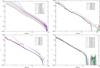 |
Fig. 1. Correlation functions of galaxies, ξ(r). Panels from top left to bottom right: LCDM models for different particle selection limits; for SDSS galaxies using five luminosity thresholds; for six luminosity bins of Millennium galaxies, and for eight luminosity thresholds of EAGLE galaxies. |
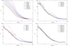 |
Fig. 2. Pair correlation or structure functions, g(r) = 1 + ξ(r). The location of the panels is the same as in Fig. 1. |
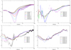 |
Fig. 3. Fractal dimension functions, D(r) = 3 + γ(r). The location of the panels is the same as in Fig. 1. Errors are found with the fit procedure, and are given for several representative samples. |
We calculated the relative correlation functions for all samples of LCDM models, which define the bias functions,
 (5)
(5)
The bias functions have a plateau 6 ≤ r ≤ 20 h−1 Mpc, see Fig. 8. This feature is similar to the plateau around k ≈ 0.03 h−1 Mpc of relative power spectra (Einasto et al. 2019). We used this plateau to measure the amplitude of the correlation function. In this separation range, the correlation functions are almost linear in log-log representation, therefore the exact location of the reference point influences our results only quantitatively, but makes little qualitative difference. Our choice was r6 = 6 h−1 Mpc. We calculated for all samples the value of the correlation function at distance (galaxy separation) r6 = 6 h−1 Mpc, ξ6; this parameter characterises the amplitude of the correlation function. It is complimentary to the correlation radius r0. At smaller distances, the correlation functions are influenced by strong non-linear effects, and at larger distances, the correlation functions for highly biased samples have wiggles, which hampers the comparison of samples with various particle density limits.
2.2. Biased model samples
The simulations of the evolution of the cosmic web were performed in a box of size L0 = 512 h−1 Mpc, with a resolution Ngrid = 512 and with  particles. The spectrum for the initial density fluctuation was generated using the COSMICS code by Bertschinger (1995), assuming concordance ΛCDM cosmological parameters (Bahcall et al. 1999): Ωm = 0.28, ΩΛ = 0.72, σ8 = 0.84, and the dimensionless Hubble constant h = 0.73. To generate the initial data, we used the baryonic matter density Ωb = 0.044 (Tegmark et al. 2004b). Calculations were performed with the GADGET-2 code by Springel (2005). The same model was used by Einasto et al. (2019) to investigate the biasing phenomenon using power spectra.
For all simulation particles and all simulation epochs, we calculated the local density values at particle locations, ρ, using the positions of the 27 nearest particles, including the particle itself. Densities were expressed in units of the mean density of the whole simulation. We formed biased model samples, selected on the particle density at the present epoch. The full ΛCDM model includes all particles. Following Einasto et al. (2019), we formed biased model samples that contained particles above a certain limit, ρ ≥ ρ0, in units of the mean density of the simulation. As shown by Einasto et al. (2019), this sharp density limit allows determining density fields of simulated galaxies whose geometrical properties are close to the density fields of real galaxies. The biased samples are denoted LCDM.i, where i denotes the particle-density limit ρ0. The full DM model includes all particles and corresponds to the particle-density limit ρ0 = 0, and therefore it is denoted as LCDM.00. The main data on the biased model samples are given in Table 1. We calculated for all samples the correlation length, r0, and the amplitude of the correlation function at r6 = 6 h−1 Mpc, ξ6 = ξ(6), all as functions of the particle density limit, ρ0.
LCDM particle-density-limited models.
The gradient of the structure function changes very rapidly at small r. For this reason, we calculated correlation functions using two resolutions, 3072 and 1024. Fractal dimension functions were calculated for the LCDM sample with resolution 3072 with different ±m steps: for r ≤ 6.5 h−1 Mpc m = 3, for 6.5 < r ≤ 17 h−1 Mpc m = 10, and thereafter m = 50. In case of the LCDM sample with resolution 1024, we used at 4.5 ≤ r ≤ 25 h−1 Mpc m = 8, thereafter m = 25. The final fractal dimension function presented in Fig. 3 is a combined function that we determined using the high-resolution field 3072 at small distances, r ≤ 8 h−1 Mpc, and the field 1024 at larger distances.
LCDM model samples are based on all particles of the simulation and contain detailed information on the distribution of matter in regions of different density. Figure 1 shows the correlation functions, ξ(r), Fig. 2 shows the structure functions, g(r) = 1 + ξ(r), and Fig. 3 shows the fractal dimension functions, D(r) = 3 + γ(r) for the basic samples of the model.
The first impression from the figure is that the amplitude of the correlation and structure functions continuously increases with increasing particle density threshold ρ0 of models. This increase can be expressed by the amplitude parameter ξ6, given in Table 1. The radius rz where the correlation function becomes negative is equal to rz ≈ 80 h−1 Mpc for all LCDM samples.
2.3. SDSS galaxy samples
We used the luminosity-limited (usually referred to as volume-limited) galaxy samples by Tempel et al. (2014a), selected from data release 12 (DR12) of the SDSS galaxy redshift survey (Ahn et al. 2014). The authors complemented the SDSS galaxy sample with redshifts from the 2MRS, 2dFGRS, and RC3 catalogues. The catalogue has a Petrosian r-band magnitude limit mr ≤ 17.77, it covers 7221 square degrees in the sky, and contains 584 450 galaxies. We used a version of the catalogue with a reduced footprint in survey coordinates −33 ° ≤η ≤ 36°, −48 ° ≤λ ≤ 51°. This version uses the most reliable data and contains 489 510 galaxies. For comparison, we note that in the study of the SDSS correlation function, Zehavi et al. (2011) used a sample of 540 000 galaxies in the magnitude interval 14.4 ≤ mr ≤ 17.6, in a footprint 7700 deg2.
The data on five luminosity-limited SDSS samples are listed in Table 2: the limiting absolute magnitudes in red r-band, Mr, the maximum comoving distances, dmax, and the numbers of galaxies in samples, Ngal. All SDSS samples have a minimum comoving distance dmin = 60 h−1 Mpc. At smaller distance, the catalogue is inhomogeneous, see Fig. 5 by Tempel et al. (2014a). The maximum comoving distances are taken from Tempel et al. (2014a); within these limits, volume-limited samples have a distance-independent number density of galaxy groups. The SDSS samples with Mr − 5 log h luminosity limits −18.0, −19.0, −20.0, −21.0, and −22.0 are referred to as SDSS.18i, SDSS.19i, SDSS.20i, SDSS.21i, and SDSS.22i, with the additional index i, where i = b is for luminosity bin samples, and i = t is for luminosity threshold samples. In luminosity bin samples, the width of the bin is one mag, ΔM = 1.0, and in luminosity threshold samples, the upper limit Mr − 5 log h = −25.0 exceeds the luminosity of the brightest galaxies in the SDSS sample. The respective luminosity limits in solar units were calculated using the absolute magnitude of the Sun in r-band, M⊙ = 4.64 (Blanton & Roweis 2007). Table 2 also provides the correlation radius of samples, r0, and the value of the correlation function at r6 = 6 h−1 Mpc, ξ6, which we used to characterise the amplitude of the correlation function.
SDSS luminosity-limited samples.
The SDSS galaxy samples are conical shells, and the corresponding random particle samples were calculated using identical conical shell configurations. The correlation functions of SDSS galaxy samples were calculated using the Landy-Szalay estimator. The SDSS samples differ from model samples in one important aspect. We used samples limited in absolute magnitude, but observational samples are flux limited. For this reason, for the faintest galaxies, only the nearby region with a distance limit dmax = 135 h−1 Mpc can be used, in contrast to the most luminous sample, for which the distance limit is dmax = 571 h−1 Mpc. The SDSS galaxy samples are conical and have different sizes: for example, the volume of sample SDSS.21 is about 50 times larger than the volume of sample SDSS.18.
To determine the behaviour of the correlation function on small distances, we used distances 0.1 ≤ r ≤ 1 h−1 Mpc using NB = 20 log bins, and on scales 0.5 ≤ r ≤ 200 h−1 Mpc using NB = 45 log bins. The fractal dimension function was calculated using the fit subroutine with m = 2 for small distances, r ≤ 1 h−1 Mpc, and m = 4 for larger distances.
The correlation functions of the SDSS galaxies are shown in Fig. 1 for the luminosity threshold, and in Fig. 4 for the luminosity bins and thresholds. The correlation functions for the luminosity bins are very similar to the correlation functions for the luminosity thresholds, but the correlation lengths are slightly lower, see Table 2. This is expected because in threshold-limited samples, brighter galaxies are included. These galaxies have larger correlation lengths.
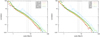 |
Fig. 4. Comparison of correlation functions of SDSS samples found for absolute magnitude bins and thresholds, left and right panels, respectively. Error bars are shown. |
The radius rz at which the correlation function becomes negative is the same for the SDSS.18 and SDSS.19 samples, rz ≈ 45 h−1 Mpc, for brighter galaxies, it lies higher, rz ≈ 120 h−1 Mpc. This difference is expected because the sample sizes for fainter galaxies are small and cannot be considered as fair samples of the universe. The structure function g(r) = 1 + ξ(r) continuously decreases with increasing distance r.
2.4. Millennium simulation galaxy samples
We used simulated galaxy catalogues by Croton et al. (2006), which are calculated based on semi-analytical models of galaxy formation from the Millennium simulations by Springel et al. (2005). The Millennium catalogue contains 8 964 936 simulated galaxies, with absolute magnitudes in r colour Mr ≤ −17.4. The magnitudes are in standard SDSS filters, not in −5 log h units. We extracted the following data: x, y, z coordinates, and absolute magnitudes in r and g photometric systems. The Millennium samples with Mr luminosity limits −18.0, −19.0, −20.0, −20.5, −21.0, −21.5, −22.0, and −23.0 are referred to as Mill.18i, Mill.19i, Mill.20i, Mill.20.5i, Mill.21i, Mill.21.5i, Mill.22i, and Mill.23i, where the index i = b is for luminosity bin samples, and i = t is for luminosity threshold samples with an upper limit −25.0. Data on the Millennium luminosity-limited samples are given in Table 3, including the correlation lengths found for Millennium galaxy samples, and the value of the correlation function at r6 = 6 h−1 Mpc, ξ6.
Millennium luminosity-limited galaxy samples.
The Millennium sample of simulated galaxies has almost nine million objects. Our first task was to calculate correlation functions for such a large dataset. We tried several possibilities: dividing the sample into smaller subsamples of 100 and 250 h−1 Mpc, and using smaller luminosity bins. Our experience shows that boxes of 250 and 500 h−1 Mpc yield almost identical results for the correlation function. The sample of 100 h−1 Mpc contains too few galaxies, which leads to larger random and some systematic errors.
One possibility to reduce the size of galaxy samples is to use smaller magnitude bins. At the low end of the luminosity range, we tried bins of 0.15, 0.25, and 0.5 in absolute magnitude. The results for the correlation function were practically identical. For samples Mill.18b and Mill.19b, we used luminosity bins 0.25 and 0.50 mag, respectively, and for the brighter samples, we used bins of 1.0 mag. The samples with threshold magnitudes at low absolute magnitudes are so large that our program for computing the correlation function was not able to manage the file. For this reason, we only calculated the correlation functions for magnitude thresholds for samples with Mr ≤ −20.0. The results are listed in Table 3. In Figs. 1–3 we show the correlation function, ξ(r), the structure function, 1 + ξ(r), and the fractal dimension function, D(r) = 3 + γ(r) for the luminosity bins. The number of simulated galaxies in most magnitude bin samples is so large that the correlation functions are very smooth with almost no scatter, thus it is easy to find the correlation length r0 and the amplitude parameter ξ6 of samples by linear interpolation. As usual, the correlation length is defined as the distance at which the correlation function has the unit value,ξ(r0) = 1.0. At this distance, the central galaxy has just one neighbour, and the density of galaxies is twice the mean density.
We calculated the correlation functions with three resolutions at distances 0.1 ≤ r ≤ 10 h−1 Mpc, 1 ≤ r ≤ 100 h−1 Mpc, and 2 ≤ r ≤ 200 h−1 Mpc, all with Nb = 100 equal linear bins of 0.1, 1, and 2 h−1 Mpc, respectively. The correlation functions presented in Fig. 1 are the results, combined from resolutions with bin sizes 0.1 and 1 h−1 Mpc, used for r ≤ 3 and r > 3 h−1 Mpc, respectively. To determine the fractal dimension function, we applied smoothing with m = 3 up to r = 10 h−1 Mpc, and m = 6 on larger distances.
Our calculation show that the correlation function of Millennium galaxies at small and medium distances has a continuously changing gradient γ(r), as found for the SDSS samples. At larger distances, the correlation function bends and crosses the zero value, ξ(rz) = 0. The radius rz where the correlation function becomes negative lies at rz = 46 ± 1 h−1 Mpc for all samples, see Fig. 1.
On large scales r ≥ rz , the correlation function lies close to the zero value. However, the baryonic acoustic oscillation (BAO) peak at r ≈ 110 h−1 Mpc is clearly visible when the function is expanded in vertical direction, as shown in Fig. 5.
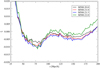 |
Fig. 5. Correlation functions on large scales of Millennium simulations for luminosity thresholds to show the BAO peak at r ≈ 110 h−1 Mpc. |
2.5. EAGLE simulation galaxy samples
The Evolution and Assembly of GaLaxies and their Environments (EAGLE) is a suite of cosmological hydrodynamical simulations that follow the formation and evolution of galaxies. Its goals are described by Schaye et al. (2015) and Crain et al. (2015). We extracted galaxy data from the public release of halo and galaxy catalogues (McAlpine et al. 2016). The EAGLE simulations were run with the following cosmological parameters: Ωm = 0.308, ΩΛ = 0.692, and H0 = 67.8 km s−1 per Megaparsec. Within the EAGLE project, several simulations were run. We used for the correlation analysis the simulation within a box of comoving size L = 100 Mpc. In contrast to convention, box sizes and lengths are not quoted in units of 1/h. This means that in conventional units, the size of the simulation box in comoving coordinates is L = 67.8 h−1 Mpc. We used x, y, z coordinates and absolute magnitudes in the r and g photometric systems.
The EAGLE samples with Mr luminosity limits −15.0, −16.0, −17.0, −18.0, −19.0, −20.0, −21.0, and −22.0 are referred to as EAGLE.15i, EAGLE.16i, EAGLE.17i, EAGLE.18i, EAGLE.19i, EAGLE.20i, EAGLE.21i, and EAGLE.22i, where the index i = b is for luminosity bin samples of a bin size of 1.0 mag, and i = t is for luminosity threshold samples with an upper limit of Mr − 5 log h = −25.0. Data on EAGLE luminosity-limited samples are given in Table 4. We also list the correlation lengths found for EAGLE galaxy samples, and the value of the correlation function at r6 = 6 h−1 Mpc, ξ6.
EAGLE luminosity-limited samples.
For the correlation analysis we used the largest simulated galaxy sample with 29 730 objects in the Mr luminosity interval −14.7 ≥ Mr ≥ −23.7. This allowed us to calculate correlation functions for luminosity bins and luminosity threshold limits starting from Mr = −15.0 up to Mr = −22.0. The data of the samples are listed in Table 4. The correlation, structure, and fractal dimension functions are presented in Figs. 1−3 for luminosity thresholds. The distance scale is expressed in h−1 Mpc.
The correlation functions of the EAGLE samples were calculated for two resolutions: at distances 0.2 ≤ r ≤ 20 Mpc and 1 ≤ r ≤ 100 Mpc, with Nb = 100 equal linear bins of size 0.2 and 1 Mpc, respectively. The correlation functions are presented in Fig. 1. High-resolution functions were used up to distance r ≤ 3 h−1 Mpc, and low-resolution functions on larger distances. To determine the fractal dimension function, we applied a smoothing with m = 3 up to r = 3 h−1 Mpc, and m = 15 on larger distances.
The shape of the correlation functions is similar to that of those for the Millennium simulation. The basic difference is that for the EAGLE simulation, it was possible to derive correlation functions for much fainter samples up to Mr = −15.0. The radius rz where the correlation function becomes negative is the same for all samples rz = 17 ± 1 h−1 Mpc. This is much smaller than for the SDSS, LCDM, and Millennium samples. This is due to the small volume of the simulation box.
2.6. Error estimations of the correlation functions
The sampling errors we found using the bootstrap method for the SDSS samples are shown in Fig. 4 for the absolute magnitude bin and the threshold samples in the left and right panels. From these data we also determined the errors of the correlation length, r0, given in Table 2. We found that the sampling errors can approximately be expressed as follows: 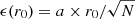 , where N is the number of galaxies in the sample, and a is a constant. The correlation lengths of SDSS galaxies behave similarly, as found by Zehavi et al. (2011). A similar relation can also be used for the errors of the correlation function amplitudes, ξ6. Using the Zehavi et al. (2011) SDSS sample and our sample, we found for the parameter the value a = 8.4. Using this relation, we estimated errors of the correlation lengths of the Millennium and EAGLE simulation samples given in tables. The relative errors of the correlation amplitudes are equal to the relative errors of the correlation lengths.
Most of our samples contain so many galaxies that the random sampling errors are very small, and the correlation and structure functions are very smooth. For this reason, the scatter of the correlation lengths, r0, and correlation amplitudes, ξ6, that we found for various luminosity limits of identical samples is also small, see Tables 1–4. The relative sampling errors of the correlation length, r0, and the correlation amplitude, ξ6, are of the order of a few percent for most samples. Samples corresponding to luminous galaxies contain fewer objects, therefore the random sampling errors of r0 and ξ6 are larger.
The number of galaxy-galaxy pairs at large distances is very large, as is the number of random-random pairs. Correlation functions were calculated based on the ratios of very large almost identical numbers. For this reason, the sampling errors of the correlation functions on large distances are larger, and larger smoothing was needed to calculate the correlation dimension functions.
3. Biasing properties of LCDM and galaxy samples
In this section we give an overview of previous determinations of the correlation functions. Next we discuss the luminosity dependence of the correlation functions and their derivatives of LCDM and galaxy samples, and the bias parameters that were found for these samples. We focus the discussion on the differences of the correlation properties in samples with real or simulated galaxies and with only DM particles.
3.1. Correlation functions of galaxies: previous studies
Classical methods for calculating angular and spatial correlation functions using catalogues of extragalactic objects were elaborated by Limber (1953, 1954), Totsuji & Kihara (1969), Peebles (1973), and Groth & Peebles (1977), see also Peebles (1980) and Martínez & Saar (2002). An analysis of almost all galaxy and cluster catalogues that were available in the 1970s (Abell 1958; Shane & Wirtanen 1967; Zwicky et al. 1968) was performed by Hauser & Peebles (1973), Peebles & Hauser (1974), Peebles & Groth (1975), Peebles (1975), Groth & Peebles (1977), and Seldner et al. (1977).
These studies showed that the spatial correlation function, calculated from the angular correlation function, can be expressed by a simple law:
 (6)
(6)
where r0 = 4.7 h−1 Mpc is the correlation length of the sample, and the power index is γ = −1.77 for the Shane-Wirtanen catalogue (Groth & Peebles 1977). Other catalogues studied yield almost the same parameters.
In the 1970s, redshift surveys of galaxies were complete enough to determine the spatial correlation functions of galaxies and galaxy clusters. To use redshift data, Peebles (1976), Davis et al. (1978), and Davis & Peebles (1983) suggested to use the galaxy position and velocity information separately. In this case, pair separations can be calculated parallel to the line of sight, π, and perpendicular to the line of sight, rp. The angular correlation function, wp(rp), can be found by integrating over the measured ξ(rp, π), using the equation
 (7)
(7)
where rmin and rmax are minimum and maximum distances of the galaxies in samples. This equation has the form of the Abel integral equation, and can be inverted to recover the spatial correlation function (Davis & Peebles 1983),
 (8)
(8)
Davis & Peebles (1983) found that the spatial correlation function can be well represented by a power law Eq. (6), with the parameters r0 = 5.4 ± 0.3 h−1 Mpc, and γ = −1.77.
Klypin & Kopylov (1983) and Bahcall & Soneira (1983) found that the correlation function of rich clusters of galaxies is similar to the correlation function of galaxies, but has a much larger correlation length. This behaviour has been predicted by Peebles & Hauser (1974). This difference was explained by Kaiser (1984) as the biasing phenomenon: rich clusters are more clustered or more biased representatives of extragalactic objects.
Einasto et al. (1986) studied the effect of voids on spatial correlation function. The authors showed that the presence of voids increases the correlation amplitude and length. This is clear from a comparison of two simple toy models: the galaxies in the models are identical, but in the void model, the sample is surrounded by an empty space. In the void sample, the same number of random points fills a larger volume, and in a given separation interval, there are fewer random points than in the first sample. This increases the correlation amplitude according to Eq. (1). Einasto et al. (1986) argued that Lick counts represent the numbers of galaxies integrated over the line of sight in the Lick maps, but voids that are present in the volume along the line of sight are filled with foreground and background objects. This causes the decrease in amplitude of the correlation functions found in 2D data. The authors also showed that the correlation length increases for more luminous galaxies.
These results were interpreted by Pietronero (1987) and Calzetti et al. (1987, 1988) as the presence of fractal structure in the universe. Hamilton (1988) confirmed the dependence of the correlation amplitude on the luminosity of galaxies. The amplitude of the correlation functions of galaxies brighter than MB relative to the amplitude at MB = −19 is almost flat for MB > −20 and rises considerably for MB < −21. He explained this as the biasing effect: luminous galaxies form in more clustered regions.
Maddox et al. (1990, 1996) measured the angular correlation function of the APM Galaxy Survey, which contains over two million galaxies in the magnitude range 17 ≤ bj ≤ 20.5 in the photometric system bj of the survey. At small separations, the angular correlation function was determined by counting individual galaxies, and on larger separations by counts of galaxies in cells of size  . Estimates of the angular correlation function w(θ) were made in six magnitude slices. The data agree well with a power law w(θ) = Aθγ − 1, where A is a constant depending on sample depth. The authors found that this power law is valid over a wide range of angular separations 0.01 ≤ θ ≤ 3 degrees, with a constant slope γ = −1.699 ± 0.032, in good agreement with Groth & Peebles (1977) for the Lick survey. The amplitude of the correlation function was calculated using the Limber equation and applying cosmological models with various parameters. The resulting correlation length varies between r0 = 4.4−5.0 h−1 Mpc, depending on the model.
Norberg et al. (2001) and Hawkins et al. (2003) used the 2dF Galaxy Redshift Survey (2dFGRS) to calculate the correlation functions of galaxies and to investigate the clustering properties of the universe. The authors analysed in detail the two-point correlation function ξ(rp, π) and its spherical average, which gives an estimate of the redshift-space correlation function, ξ(s), where s is the separation of galaxies in redshift space. As the first step, the authors measured the 2D correlation function ξ(rp, π), and integrated over the line of sight using Eq. (7) to avoid supercluster contraction effects (Kaiser 1987). The authors found that the effective depth of the 2dFGRS is zs ≈ 0.15, the effective luminosity Ls ≈ 1.4L⋆, the redshift-space clustering length is s0 = 6.82 ± 0.28 h−1 Mpc, and the real-space correlation length is r0 = 5.05 ± 0.26 h−1 Mpc. Norberg et al. (2001) found for the relative bias function of galaxies b/b* = 0.85 + 0.15L/L⋆, which agrees well with Hamilton (1988).
Zehavi et al. (2004, 2005, 2011) studied the luminosity dependence of the correlation functions using flux-limited and volume-limited samples of SDSS galaxies. The authors measured the projected 2D correlation function wp(rp). In the first step, the authors calculated ξ(rp, π) by counting data-data, data-random, and random-random pairs using the Landy-Szalay estimator Eq. (2). Next, the authors computed the projected correlation functions wp(rp) using Eq. (7), and adopting rmin = 0 and rmax = 40 h−1 Mpc. Zehavi et al. (2011) found for the large-scale bias function the form bg(> L)×(σ8/0.8) = 1.06 + 0.21(L/L*)1.12, where L is the r-band luminosity corrected to z = 0.1, and L* corresponds to M* = −20.44 ± 0.01 (Blanton et al. 2003).
Zehavi et al. (2004, 2005, 2011) concentrated their effort on investigating the profile of the correlation function. The authors used for comparison a ΛCDM model by applying the halo occupation distribution (HOD) model by Peacock & Smith (2000), Seljak (2000), and Berlind & Weinberg (2002). The authors assumed that halos have a Navarro-Frenk-White (NFW) profile (Navarro et al. 1996), and are populated with galaxies that trace the DM profile. The authors found that correlation functions of HOD models and luminosity-limited SDSS samples change in the slope of the correlation function at r ≈ 2 h−1 Mpc. On a smaller scale, the one-halo contribution dominates, and on a larger scale, the galaxies from different halos dominate. We note that this effect has been described by Zeldovich et al. (1982) and by Einasto (1991a, 1992) using galaxy data. Einasto (1992) found that the transition from clusters to filaments with different values of the slope of the correlation function is rather sharp: γ = −1.8 for r < 3 h−1 Mpc, and γ = −0.8 for larger scales. This sharp transition was confirmed by Zehavi et al. (2004) on the basis of the HOD model.
We compare in Fig. 6 the correlation lengths of SDSS samples of various luminosity. Zehavi et al. (2011) found spatial correlation functions from projected correlation functions as described above. Our correlation functions were calculated directly from 3D data. Here two trends are clearly visible: the dependence of the correlation lengths on the galaxy luminosity, and the overall shift of the amplitudes of 3D correlation functions with respect to the correlation functions from a 2D analysis. The luminosity dependence of 2D and 3D samples is similar. The general shift of the amplitudes of the 3D correlation functions with respect to 2D samples arises because in 3D samples, the regions of zero spatial density are taken into account and increase the amplitude of the correlations functions. In a 2D analysis, the presence of voids is ignored. The correlation lengths of SDSS galaxies in identical luminosity limits are according to our 3D analysis in the mean 1.35 times higher than according to the 2D analysis by Zehavi et al. (2011).
 |
Fig. 6. Correlation length r0 of SDSS galaxies according to 2D data by Zehavi et al. (2011) and 3D data in this paper, using luminosity thresholds samples. |
3.2. Luminosity dependence of the correlation functions of the SDSS, Millennium, and EAGLE samples
The luminosity dependence of the correlation functions is the principal factor of the biasing phenomenon, as discussed by Kaiser (1984). Here we compare the luminosity dependence of the correlation functions of real and simulated galaxies, as found in the present analysis.
Our first task was to compare the clustering properties of real SDSS galaxy samples with clustering properties of simulated galaxies of the EAGLE and Millennium simulations. As noted above, in simulations, the absolute galaxy magnitudes were not computed in −5 log h units. To compare the correlation functions of simulated and real samples, the simulated galaxy data must be reduced to real galaxy data in terms of luminosities. The simulated galaxy samples of the EAGLE and Millennium models for various luminosity limits have spatial densities that differ from the spatial densities of SDSS samples for these luminosity limits. To bring model galaxy samples to the same system as SDSS samples, the luminosities of the simulated galaxies must be weighted on the basis of the comoving luminosity densities of samples. A similar procedure was applied by Liivamägi et al. (2012) to reduce the luminosity scale of luminous red giants (LRG) to the main sample of SDSS galaxies. We found comoving spatial densities of galaxies for all SDSS, EAGLE, and Millennium subsamples for various luminosity limits. The comparison of densities shows that in order to bring spatial densities of simulated galaxies to the same density level as that of the SDSS galaxies, the luminosities of the weighted EAGLE simulation samples must be decreased by shifting the absolute magnitudes toward fainter magnitudes by 0.38 mag. The decrease in magnitudes of the Millennium simulation samples is 0.80 mag. To obtain identical spatial densities, the shift is slightly luminosity dependent, but we ignored this difference and used identical shifts for all samples of galaxies of the same simulation.
The correlation lengths for luminosity bin samples were calculated for bins of 1 mag. The correlation lengths listed in Table 2 correspond to galaxies that are 0.5 mag brighter than given in Col. (2), thus the correlation length of L⋆ galaxies is practically equal to the correlation length of the sample SDSS.20b with mean magnitude, Mr = −20.5, very close to the magnitude of L⋆ galaxies, M* = −20.44. Thus we accept using data from Table 2, r0(L⋆) = 7.20 ± 0.19. We note that this value is rather close to the value of the mean redshift space correlation length for 2dFGRS galaxies, s0 = 6.83 ± 0.28 (Hawkins et al. 2003).
In Fig. 7 we show the correlation lengths, r0, of the SDSS, EAGLE, and Millennium samples as functions of magnitude Mr. The correlation length r0 has a rather similar luminosity dependence for all samples. The correlation lengths and amplitudes of the SDSS samples are slightly higher than in the simulated galaxy samples, by a factor of about 1.2.
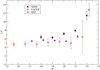 |
Fig. 7. Correlation length r0 of SDSS galaxies. For comparison, we also show the correlation lengths of the EAGLE and Millennium simulations for the luminosity bins. |
An important detail in the luminosity dependence is the fact that the correlation lengths and amplitudes are almost constant at low luminosities, M ≥ −20.0. This tendency was noted earlier by Einasto et al. (1986), Hamilton (1988), Norberg et al. (2001), and Zehavi et al. (2005, 2011). It is seen in observational samples SDSS.19 and SDSS.18, but cannot follow to fainter luminosities because very faint galaxies are absent from SDSS luminosity-limited samples. In the EAGLE and Millennium model galaxy samples, this very slow decrease of r0 and ξ6 with decreasing luminosity can be followed until very faint galaxies, M ≈ −15.6 for the EAGLE sample, and M ≈ −17.2 for the Millennium sample. This tendency indicates that very faint galaxies follow the distribution of brighter ones, that is, faint galaxies are satellites of bright galaxies. The tendency of the clustering dwarf galaxies to form satellites of brighter galaxies has been known for a long time (Einasto et al. 1974a), see also Wechsler & Tinker (2018). The correlation study confirms this tendency.
3.3. Bias parameters of the LCDM and SDSS samples
In Fig. 8 we present the bias functions (relative correlation functions) b(r, ρ0) for a series of LCDM models with various particle density limits ρ0. They were calculated using Eq. (5) for the whole range of distances r (galaxy separations) by dividing the correlation functions of the biased models LCDM.i by the correlation function of the unbiased model LCDM.00. The bias functions for the same biased LCDM models were calculated from power spectra by Einasto et al. (2019), see Fig. 2 of this paper. Figure 8 shows that the bias function has a plateau at r6 ≈ 6 h−1 Mpc, similar to the plateau around k ≈ 0.03 h−1 Mpc of the relative power spectra (Einasto et al. 2019). Both plateaus were used to determine the amplitudes of the correlation functions or power spectra to define the respective bias parameters. The figure shows that the amplitude of the correlation functions at small distances (pair separations) rises rapidly with the increase in particle density limit ρ0.
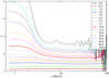 |
Fig. 8. Bias functions, b(r), of biased LCDM models as functions of the galaxy pair separation r. Particle density limits ρ0 are indicated as symbol labels. |
Figure 8 shows that bias function, b(r), for low values of the particle density threshold, ρ0 ≤ 3, is almost constant. This suggests that the correlation functions of faint galaxies are almost parallel to the correlation function of matter. The only difference is in the amplitude. At these low values of the particle density threshold ρ0, the bias parameter is essentially determined by the fraction of matter in the clustered population, that is, matter, associated with galaxies. This property allows us to derive absolute bias parameters of the biased model samples with respect to matter, as given in Table 1. As expected, the bias parameters found for the correlation functions are very close to the bias parameters of the same model that were derived from power spectra by Einasto et al. (2019). For a more detailed discussion of the effect of low-density regions of the density field of matter on the correlation function and power spectrum, see Einasto et al. (1993, 1994, 1999).
In Fig. 9 we show the relative bias function b(L)/b(L*) for galaxies of various luminosity of the SDSS, EAGLE, and Millennium samples. The relative bias function was calculated from the relation
 (9)
(9)
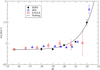 |
Fig. 9. Relative bias function b(L)/b(L*) for the SDSS, EAGLE, and Millennium samples. The solid line shows the relative bias function by Norberg et al. (2001). |
using amplitudes of the correlation functions at the plateau at r6 = 6 h−1 Mpc of samples of luminosity L, divided by the amplitudes of the correlation functions at r6 = 6 h−1 Mpc of the same sample at luminosity L*. This representation is commonly used, here L* is the characteristic luminosity of the samples. It corresponds approximately to the red magnitude Mr = −20.5. The relative bias function rises rapidly with the increase in luminosity over L*. This increase in the relative bias function at high luminosities has been observed by Einasto et al. (1986), Hamilton (1988), Norberg et al. (2001), Tegmark et al. (2004a), and Zehavi et al. (2005, 2011). Figure 9 shows that within the errors, the relative bias function of the SDSS sample agrees with the relative bias function by Norberg et al. (2001). Deviations of the Millennium and EAGLE relative correlation functions from the Norberg fit are slightly larger, but within reasonable limits.
Table 1 shows the bias parameter b(ρ0) of the LCDM model as a function of ρ0. This bias parameter relates biased models with unbiased models, that is, relative to all matter. The bias parameter increases continuously with the increase in threshold ρ0, in contrast to the relative bias parameters of the observational and the model EAGLE and Millennium galaxy samples, that is, the bias parameters of L galaxies with respect to L* galaxies, which have flat r0(M) and ξ6(M) curves at low luminosities.
This difference can be explained by differences in the distribution of DM particles and dwarf galaxies. Removing low-density particles from the LCDM sample with increasing ρ0 limit affects the distribution of high-density regions (clusters in terms of the percolation analysis by Einasto et al. 2018) over the whole volume of the LCDM model. Removing very faint dwarf galaxies form real SDSS or simulated EAGLE and Millennium galaxy samples only affects the structure of halos that contain brighter galaxies, but not the structure of voids because voids do not contain isolated dwarf galaxies. This difference is rather small and does not affect the overall geometrical properties of the cosmic web of real and model samples, as measured by the extended percolation analysis by Einasto et al. (2019). However, the correlation function is sensitive enough to detect this small difference in the spatial distribution of dwarf galaxies and DM particles in low-density regions.
3.4. Correlation function amplitudes of the LCDM and SDSS samples
The amplitudes of the correlation functions of the biased LCDM samples are systematically higher than respective amplitudes of the SDSS galaxy samples, see Tables 1 and 2 and Fig. 7. A comparison of the percolation properties of SDSS and LCDM samples showed that LCDM models with a particle density threshold limits 3 ≤ ρ0 ≤ 10 correspond approximately to SDSS samples with absolute magnitude limits −18.0 ≥ Mr ≥ −21.0 (Einasto et al. 2018). Within these selection parameter limits, the correlation amplitudes of biased LCDM samples can be reduced to the amplitude levels of SDSS samples using an amplitude reduction factor 0.65. The reason for this difference is not clear. One possibility is that our LCDM model has a different σ8 normalisation than real SDSS data.
Figure 10 shows the correlation functions of the SDSS samples together with the reduced correlation functions of the biased model samples LCDM.3, LCDM.10, and LCDM.80, as well as the correlation function of the whole matter LCDM.00, shown in the figure by the black bold dashed line. At medium and large scales, r ≥ 3 h−1 Mpc, the correlation function of the SDSS.22t sample is very close to the correlation function of the biased model sample LCDM.80. Similarly, the correlation functions of the SDSS.20t and SDSS.21t samples are close to the correlation function of the LCDM.10 sample, and the correlation functions of the SDSS.18t and SDSS.19t samples are close to the correlation function of the LCDM.3 sample. The correlation functions of last two SDSS samples bend down at a distance r ≥ 40 h−1 Mpc, and deviate on larger scales from those of the LCDM samples. This deviation is due to smaller volumes in the SDSS.18 and SDSS.19 samples, similarly to the behaviour of the correlation functions of the EAGLE simulation galaxies.
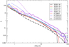 |
Fig. 10. Correlation functions of SDSS galaxies compared with the reduced correlation functions of LCDM samples, using a reduction factor of 0.65. |
On smaller scales r ≤ 3 h−1 Mpc, the correlation functions of the LCDM samples have a higher amplitude than the correlation functions of the corresponding SDSS samples. As discussed above, in this distance range, the correlation functions of the LCDM models reflect the internal structure of the DM halos. Inside the DM halos, the density of the DM particles is very high, and all DM particles are present in our samples. This explains the rise of the correlation function of the LCDM samples. The number density of visible galaxies in our luminosity-limited galaxy samples does not follow this tendency because most satellite galaxies and cluster members are fainter than the luminosity limit.
4. Fractal properties of the cosmic web
In this section we discuss the fractal properties of the cosmic web as measured by the correlation function and its derivatives. The LCDM samples differ from the SDSS, Millennium, and EAGLE samples in one principal factor: in the LCDM samples, individual DM particles are present, but in real and simulated galaxy samples, only galaxies brighter than a certain limit are present. This difference affects the correlation functions and their derivatives, the structure and gradient functions. The largest difference is in the fractal dimension functions, which contain information on the distribution of the DM particles within halos, as well as on the distribution of the DM halos and galaxies in the cosmic web.
4.1. Fractal dimension properties of the LCDM models
One aspect of the structure of the cosmic web is its fractal character. The fractal geometry of various objects in nature was discussed by Mandelbrot (1982). The study of fractal properties of the cosmic web has a long history. The first essential step for studying fractal properties of the cosmic web was made by Soneira & Peebles (1978). The authors constructed a fractal model that allowed reproducing the angular correlation function of the Lick catalogue of galaxies, as found by Seldner et al. (1977). Over a wide range of mutual separations (distances), 0.01 ≤ r ≤ 10 h−1 Mpc, the correlation function can be represented by a power law, ξ(r) = (r/r0)γ, where r0 = 4.5 ± 0.5 h−1 Mpc is the correlation length, γ = −1.77 is a characteristic power index, and D = 3 + γ = 1.23 ± 0.04 is the fractal dimension of the sample (Peebles 1989, 1998).
Subsequent studies have shown that the cosmic web has a multifractal character, as found by numerous authors, starting from Jones et al. (1988), and confirmed by Balian & Schaeffer (1988), Martinez et al. (1990, 1993), Einasto (1991a), Guzzo et al. (1991), Colombi et al. (1992), Borgani (1995), Mandelbrot (1997), Baryshev et al. (1998), Gaite et al. (1999), Bagla et al. (2008), Chacón-Cardona & Casas-Miranda (2012), and Gaite (2018, 2019). In these pioneering studies, the fractal character of the web was studied mostly locally in samples of different sizes, as discussed by Martínez & Saar (2002).
Einasto (1991b, 1992) and Guzzo et al. (1991) showed that at separations r < 3 h−1 Mpc, the correlation function of galaxies reflects the galaxy distrubution in groups and clusters, and at larger distances, the intracluster distribution (up to ∼30 h−1 Mpc). This was confirmed by Berlind & Weinberg (2002), Zehavi et al. (2004), and Kravtsov et al. (2004), who noted that at small mutual separations r, the correlation function characterises the distribution of matter within DM halos, and on larger separations, the distribution of halos. In the small separation region, the spatial correlation function of the LCDM model samples is proportional to the density of matter, and measures the density profile inside the DM halos. The upper left panel of Fig. 3 shows that the fractal dimension function of the LCDM samples strongly depends on the particle density limit ρ0 that is used in selecting particles for the sample.
All LCDM samples at a distance r = 0.5 h−1 Mpc have an identical value of the gradient function, γ(0.5) = − 1.5, and of the respective local fractal dimension, D(0.5) = 1.5. At a distance of about 2 h−1 Mpc, the gradients have a minimum that depends on the particle density limit ρ0 of the samples, see Table 5. After the minimum, the gradient function increases and reaches the expected value γ(100)≈0 (D(100)≈3.0) for all samples at the largest distance.
Minima of the gradient functions of the LCDM models.
The identical values of the gradient functions at r = 0.5 h−1 Mpc, followed by a minimum at r ≈ 2 h−1 Mpc, depending on the particle density limit of the LCDM samples, can be explained by the internal structure of the DM halos. It is well known that DM halos have almost identical DM density profiles, which can be described by the NFW (Navarro et al. 1996) and by the Einasto (1965) profile. As shown by Wang et al. (2019), the density of DM halos is better fitted by the Einasto profile,
![Mathematical equation: $$ \begin{aligned} \rho (r) = \rho _{-2} \exp [-2\,\alpha ^{-1} ((r/r_{-2})^\alpha -1)], \end{aligned} $$](/articles/aa/full_html/2020/08/aa37683-20/aa37683-20-eq16.gif) (10)
(10)
where r−2 is the radius at which the logarithmic slope is −2, and α is a shape parameter. Wang et al. (2019) showed that density profiles of halos of very different mass are almost identical over a very wide range of halo masses, and have the shape parameter value α = 0.16. The authors calculated the logarithmic density slope d log ρ/d log r of the density profile over a distance range 0.05 ≤ r/r−2 ≤ 30. Near the halo centre, r/r−2 = 0.2, the logarithmic slope is d log ρ/d log r = −1.5, and it decreases to d log ρ/d log r = −3.0 at r/r−2 = 10 near the outer boundary of the halo.
At small distances, the correlation functions are the mean values of the sums of the particle mutual distances within the DM halos, averaged over the whole volume of the samples. At the very centre, all DM halos have identical density profiles, which explains the constant value, γ(0.5) = − 1.5. The DM halos of different mass have different sizes, thus the outer boundaries of the halos occur at various distances r, depending on the halo mass. In the full sample LCDM.00, small DM halos dominate, and the minimum of the gradient function γ(r) has a moderate depth. With increasing particle density limit ρ0, low-density halos are excluded from the sample and more massive halos dominate. This leads to an increase in depth of the minimum of γ(r) and D(r) functions. More massive halos have larger radii, thus the location of the minimum of the γ(r) function shifts to higher distance r values. More massive halos also have a higher density, thus the minimum of the γ(r) function is deeper. The r = rmin can be considered as the effective radius of the dominating DM halos of the sample.
After the minimum at higher r values, the distribution of DM particles outside the halos dominates. This leads to an increase in the γ(r) function. In these regions, the distribution of the DM particles of the whole cosmic web determines the correlation function and its derivatives. Figures 2 and 3 of Zehavi et al. (2004) show that the transition from one DM halo to the general cosmic web occurs at r ≈ 2 h−1 Mpc, which agrees well with the characteristic sizes of DM halos. We conclude that correlation functions of our biased LCDM models describe in a specific way the internal structure of DM halos, and also the fractal dimension properties of the whole cosmic web.
4.2. Fractal dimension properties of the galaxy samples
The SDSS samples have at low r values a large scatter of γ(r) and D(r) functions. The mean value of the fractal dimension function at r ≈ 0.2 is about 1.5, which is similar to the value for the LCDM samples. With increasing distance r, the γ(r) and D(r) functions decrease and have a minimum at about rmin ≈ 0.8 h−1 Mpc. The minimum is deeper for the brightest galaxies of sample SDSS.21. Thereafter, with increasing r, the γ(r) and D(r) functions increase rapidly up to D(3)≈2 (γ(3) = − 1), which corresponds to the fractal dimensions of sheets. At a still larger distance between galaxy pairs r, the γ(r) function smoothly approaches a value γ(r) = 0 at large r, as expected for a random distribution of galaxies with a fractal dimension D = 3.
The fractal functions of the Millennium and EAGLE simulation samples start at low r-values at γ(r)≈ − 1.5, D(r)≈1.5, also with a large scatter. For the two simulated galaxy samples, the fractal dimension functions have a minimum at rmin ≈ 1.5 h−1 Mpc. The minimum is deeper for brighter galaxies. A gradual increase in fractal dimension up to D = 3 at large distance follows.
The fractal dimension functions of the LCDM and galaxy samples differ in two important details: (i) at small distances, r ≈ 0.5 h−1 Mpc, the LCDM samples have an identical gradient, γ(0.5) = − 1.5, all galaxy samples in this distance region have large scatter of the gradient; (ii) the transition from halos (clusters) to the web occurs at different scales, rmin ≈ 2 h−1 Mpc for the LCDM models, rmin ≈ 0.8 h−1 Mpc for real galaxies, and rmin ≈ 1.5 h−1 Mpc for simulated galaxies. These small differences show that the internal structure of the DM halos of the LCDM models differs from the internal structure of galaxy clusters. In our biased LCDM model samples, all DM particles with density labels ρ ≥ ρ0 are present. Thus we see the whole density profile of the halos up to the outer boundary of the halo. In the real and simulated galaxy samples, only galaxies brighter than the selection limit are present. This means that in most luminous galaxy samples, only one or a few brightest galaxies are located within the visibility window, and the true internal structure of clusters up to their outer boundary is invisible. This difference is larger for real galaxies.
This result is valid not only for rich clusters of galaxies. Ordinary galaxies of the type of our Galaxy and M 31 are surrounded by satellite galaxies such as the Magellanic Clouds and dwarf galaxies encircling the Galaxy, and M 32 and dwarf galaxies around M 31. According to the available data, all ordinary galaxies have such satellite systems (Einasto et al. 1974a; Wechsler & Tinker 2018). However, the luminosity of most satellites is so low that they are invisible in galaxy surveys such as the SDSS. For this reason, the distribution of DM and visible matter within Galaxy-type halos is different, as noted previously in the early study by Einasto et al. (1974b). Groups and clusters of galaxies have more bright member galaxies, but at large distances, fainter group members also become invisible. With increasing distance, the number of visible galaxies in clusters therefore decreases, and at a large distance, only the brightest galaxy has a luminosity that is high enough to fall into the visibility window of the survey, see Fig. 9 of Tempel et al. (2009).
Cross sections of spatial 3D density fields of the SDSS and LCDM samples are shown in Fig. 14 of Einasto et al. (2019). Throughout the entire area of the cross sections of the 3D fields, small isolated spots exist. These spots correspond to primary galaxies of groups (clusters), where satellite galaxies lie outside the visibility window, or the number of members in groups is considerably reduced. In the calculation of the correlation functions, these groups enter as isolated galaxies of the field without any nearby galaxies, or as part of groups with only a few member galaxies.
The difference in spatial distribution of galaxies and matter at sub-megaparsec scales is the principal reason for the difference between the correlation functions of the LCDM and SDSS samples at small separations. The visible matter in Galaxy-type halos is concentrated in the central main galaxy. The luminosities of satellite galaxies are so low that they contribute little to the distribution of luminous matter. In contrast, DM has a smooth distribution within the halos over the whole volume of the halo up to its outer boundary.
The correlation functions of the LCDM models with the highest particle selection limit ρ0 have a bump at r ≈ 8 h−1 Mpc that causes small wiggles in the fractal dimension function. Similar features are also seen in the correlation functions of the most luminous galaxies in real and simulated galaxy samples. Less massive clusters (halos) have smoother profiles and distributions, and these features are hidden in the large body of all galaxies. A similar feature was detected by Tempel et al. (2014b) for the correlation function of galaxies, and was explained by a regular displacement of groups along filaments. See also the regular location of clusters and groups in the main cluster chain of the Perseus-Pisces supercluster (Jõeveer et al. 1977, 1978).
4.3. Dependence of fractal properties on the sample size
One of the first comparisons of the spatial correlation functions of real and model samples was made by Zeldovich et al. (1982). Figure 2 of this paper compares the correlation functions of the observed sample around the Virgo cluster with the correlation functions based on the Soneira & Peebles (1978) hierarchical clustering model, and with the hot dark matter (HDM) simulation by Doroshkevich et al. (1982). The observed correlation function has a bend at a scale r ≈ 3 h−1 Mpc. On smaller scales, the slope of the correlation function is γ(r)≈ − 3 (fractal dimension D(r)≈0), which is also present in the HDM model. On a larger scale, the slope is much shallower in the observational and in the HDM model samples. A rapid change in the slope of the correlation function of observational samples at this scale was confirmed by Einasto (1991a,b, 1992), Guzzo et al. (1991), Einasto et al. (1997c), and Zehavi et al. (2005). The authors emphasised that on smaller scales, the slope of the structure function, γ(r), lies between −1.6 and −2.25, corresponding to fractal dimensions D(r) = 1.4 to 0.5, and reflecting the distribution of the galaxies in groups and clusters. At larger distances, the slope of this function is about −0.8 and reflects the inter-cluster distribution with a fractal dimension D ≈ 2.2.
We here studied the spatial distribution of real and simulated samples with sizes of 100 to 500 h−1 Mpc. In earlier studies, samples of smaller size were available, and the contrast between clusters and filaments characterised the structure of one or a few superclusters. In larger samples, the contrast between clusters and filaments is averaged over many superclusters, and we see the characteristic behaviour of the whole cosmic web.
One aspect of the fractal character is the dependence of the correlation length on the size of the sample. Einasto et al. (1986) investigated the effect of voids on the distribution of galaxies and found that the correlation length of galaxy samples increases with the increase in size of the sample. Pietronero (1987) and Calzetti et al. (1987, 1988) explained that this result is evidence for the fractal character of the galaxy distribution. Martínez et al. (2001) investigated the increase in the correlation length with sample depth in more detail. The authors found that the correlation length increases with sample depth up to 30 h−1 Mpc, using a fractal that was constructed according to the Soneira & Peebles (1978) model. However, in real galaxy samples of increasing depth over 60 h−1 Mpc, there is no increase in the correlation length with depth.
Another important aspect of the fractal character of the cosmic web is its structure at sub-megaparsec scales, which is created by the tiny filamentary web of the DM with sub-voids, sub-sub-voids, etc, as discussed, among others, by Aragon-Calvo et al. (2010a,b) and Aragon-Calvo & Szalay (2013). We used a spatial resolution of the order of one megaparsec or slightly lower, therefore the fine details of the structure of the DM filamentary web on smaller scales are invisible.
5. Summary
This paper and accompanying papers (Einasto et al. 2019, 2020) address the biasing phenomenon and the multifractal character of the cosmic web. The biasing problem was recognised simultaneously with the detection of the cosmic web. Jõeveer et al. (1977, 1978) noted that “it is very difficult to imagine a process of galaxy and supercluster formation which is effective enough to evacuate completely such large volumes as cell interiors are”. As noted in the Introduction, there are two trends concerning the value of the bias parameter, either b ≈ 1, that is, galaxies follow matter, or b ≈ 2, that is, galaxies follow matter only in over-density regions, but not in voids. The bias value b ≈ 1 was based in most cases on measuring angular correlation functions, ξ(rp, π), and integrating over the line of sight π to obtain the projected correlation function wp(rp), Eq. (7). This treatment ignores the filamentary character of the cosmic web, however. In projection, clusters and filaments fill in the voids along the line of sight, which leads to the decrease in amplitude of the correlation functions (and power spectra), and to the respective bias parameters (Einasto et al. 2020).
To estimate the large-scale bias parameter in a quantitative way, we used a biased ΛCDM model and calculated power spectra, and projected and spatial correlation functions of the biased models (Einasto et al. 2019, 2020). To compare the models with observations, we developed the extended percolation method (Einasto et al. 2018). We also analysed the physical processes that cause the bias phenomenon (Einasto et al. 2019). The general results of this series of studies are summarised below.
-
The combination of several physical processes (e.g. the formation of halos along caustics of particle trajectories, and the phase synchronisation of density perturbations on various scales) transforms the initial random density field to the current highly non-random density field.
-
Because galaxy formation depends on the local density of matter, regions exist that are devoid of galaxies. These regions fill a large fraction of space in the universe. This is the main reason for the rise in amplitude of the correlation functions and power spectra of galaxies, and it increases the large-scale bias parameter.
-
The combined evidence leads to a large-scale bias parameter of L⋆ galaxies with a value b⋆ = 1.85 ± 0.15.
-
We find for the correlation length of L⋆ galaxies the value of r0(L⋆) = 7.20 ± 0.19.
We calculated for the biased ΛCDM models and for real and simulated galaxy samples the spatial correlation functions of galaxies, and their derivatives, structure functions, and fractal dimension functions. The correlation function and its derivatives are sensitive to the spatial distribution of galaxies in the cosmic web as well as to particles within DM halos. Our conclusions about the fractal nature of the cosmic web are listed below.
-
In the biased DM models, the correlation functions at small distances (separations) describe the distribution of particles in DM halos, as given by the halo density profiles. The transition from halo to web properties occurs at distance r ≈ 2 h−1 Mpc. In galaxy samples, only the brightest galaxies in clusters are visible, and the transition from clusters to filaments occurs at distance r ≈ 0.8 h−1 Mpc for real and at r ≈ 1.5 h−1 Mpc for simulated galaxies. At larger separations, the correlation functions describe the distribution of matter and galaxies in the whole cosmic web.
-
The effective fractal dimension of the cosmic web is a continuous function of distances (particle and galaxy separations). At small separations, r ≤ 2 h−1 Mpc, the gradient function decreases from γ(r)≈ − 1.5 to γ(r)≈ − 3, reflecting the particle (galaxy) distribution inside halos (clusters). The minimum of the fractal dimension function D(r) near r ≈ 2 h−1 Mpc is deeper for more luminous galaxies. At medium separations, 2 ≤ r ≤ 10 h−1 Mpc, the fractal dimension grows from ≈0 to ≈2 (filaments to sheets), and approaches 3 at large separations (random distribution).
-
Real and simulated galaxies of low luminosity, Mr ≥ −19, have almost identical correlation lengths and amplitudes. This is a strong argument indicating that dwarf galaxies are satellites of brighter galaxies, and do not form a smooth population in voids.
Acknowledgments
Our special thanks are to Enn Saar for providing a very efficient code to calculate the correlation function and for many stimulating discussions, to Ivan Suhhonenko for calculation the ΛCDM model used in this paper, and to the anonymous referee for useful suggestions. This work was supported by institutional research fundings IUT26-2 and IUT40-2 of the Estonian Ministry of Education and Research, and by the Estonian Research Council grant PRG803. We acknowledge the support by the Centre of Excellence “Dark side of the Universe” (TK133) financed by the European Union through the European Regional Development Fund. The study has also been supported by ICRAnet through a professorship for Jaan Einasto. We thank the SDSS Team for the publicly available data releases. Funding for the SDSS and SDSS-II has been provided by the Alfred P. Sloan Foundation, the Participating Institutions, the National Science Foundation, the US Department of Energy, the National Aeronautics and Space Administration, the Japanese Monbukagakusho, the Max Planck Society, and the Higher Education Funding Council for England. The SDSS Website is http://www.sdss.org/. The SDSS is managed by the Astrophysical Research Consortium for the Participating Institutions. The Participating Institutions are the American Museum of Natural History, Astrophysical Institute Potsdam, University of Basel, University of Cambridge, Case Western Reserve University, University of Chicago, Drexel University, Fermilab, the Institute for Advanced Study, the Japan Participation Group, Johns Hopkins University, the Joint Institute for Nuclear Astrophysics, the Kavli Institute for Particle Astrophysics and Cosmology, the Korean Scientist Group, the Chinese Academy of Sciences (LAMOST), Los Alamos National Laboratory, the Max-Planck-Institute for Astronomy (MPIA), the Max-Planck-Institute for Astrophysics (MPA), New Mexico State University, Ohio State University, University of Pittsburgh, University of Portsmouth, Princeton University, the United States Naval Observatory, and the University of Washington.
References
- Abell, G. O. 1958, ApJS, 3, 211 [NASA ADS] [CrossRef] [Google Scholar]
- Ahn, C. P., Alexandroff, R., Allende Prieto, C., et al. 2014, ApJS, 211, 17 [NASA ADS] [CrossRef] [Google Scholar]
- Aragon-Calvo, M. A., & Szalay, A. S. 2013, MNRAS, 428, 3409 [NASA ADS] [CrossRef] [Google Scholar]
- Aragon-Calvo, M. A., van de Weygaert, R., Araya-Melo, P. A., Platen, E., & Szalay, A. S. 2010a, MNRAS, 404, L89 [NASA ADS] [CrossRef] [Google Scholar]
- Aragon-Calvo, M. A., van de Weygaert, R., & Jones, B. J. T. 2010b, MNRAS, 408, 2163 [NASA ADS] [CrossRef] [Google Scholar]
- Bagla, J. S., Yadav, J., & Seshadri, T. R. 2008, MNRAS, 390, 829 [NASA ADS] [CrossRef] [Google Scholar]
- Bahcall, N. A., & Soneira, R. M. 1983, ApJ, 270, 20 [NASA ADS] [CrossRef] [Google Scholar]
- Bahcall, N. A., Ostriker, J. P., Perlmutter, S., & Steinhardt, P. J. 1999, Science, 284, 1481 [NASA ADS] [CrossRef] [Google Scholar]
- Balian, R., & Schaeffer, R. 1988, ApJ, 335, L43 [NASA ADS] [CrossRef] [Google Scholar]
- Baryshev, Y. V., Sylos Labini, F., Montuori, M., Pietronero, L., & Teerikorpi, P. 1998, Fractals, 6, 231 [NASA ADS] [CrossRef] [Google Scholar]
- Berlind, A. A., & Weinberg, D. H. 2002, ApJ, 575, 587 [NASA ADS] [CrossRef] [Google Scholar]
- Bertschinger, E. 1995, ArXiv e-prints [arXiv:astro-ph/9506070] [Google Scholar]
- Blanton, M. R., & Roweis, S. 2007, AJ, 133, 734 [NASA ADS] [CrossRef] [Google Scholar]
- Blanton, M. R., Hogg, D. W., Bahcall, N. A., et al. 2003, ApJ, 592, 819 [NASA ADS] [CrossRef] [Google Scholar]
- Borgani, S. 1995, Phys. Rep., 251, 1 [CrossRef] [Google Scholar]
- Calzetti, D., Einasto, J., Giavalisco, M., Ruffini, R., & Saar, E. 1987, Ap&SS, 137, 101 [NASA ADS] [CrossRef] [Google Scholar]
- Calzetti, D., Giavalisco, M., & Ruffini, R. 1988, A&A, 198, 1 [Google Scholar]
- Chacón-Cardona, C. A., & Casas-Miranda, R. A. 2012, MNRAS, 427, 2613 [CrossRef] [Google Scholar]
- Colombi, S., Bouchet, F. R., & Schaeffer, R. 1992, A&A, 263, 1 [NASA ADS] [Google Scholar]
- Crain, R. A., Schaye, J., Bower, R. G., et al. 2015, MNRAS, 450, 1937 [NASA ADS] [CrossRef] [Google Scholar]
- Croton, D. J., Springel, V., White, S. D. M., et al. 2006, MNRAS, 365, 11 [NASA ADS] [CrossRef] [Google Scholar]
- Davis, M., & Peebles, P. J. E. 1983, ApJ, 267, 465 [NASA ADS] [CrossRef] [Google Scholar]
- Davis, M., Geller, M. J., & Huchra, J. 1978, ApJ, 221, 1 [NASA ADS] [CrossRef] [Google Scholar]
- Doroshkevich, A. G., Shandarin, S. F., & Zeldovich, I. B. 1982, Comments Astrophys., 9, 265 [NASA ADS] [Google Scholar]
- Einasto, J. 1965, Trudy Astrofizicheskogo Instituta Alma-Ata, 5, 87 [NASA ADS] [Google Scholar]
- Einasto, M. 1991a, MNRAS, 252, 261 [NASA ADS] [CrossRef] [Google Scholar]
- Einasto, M. 1991b, MNRAS, 250, 802 [NASA ADS] [CrossRef] [Google Scholar]
- Einasto, M. 1992, MNRAS, 258, 571 [NASA ADS] [CrossRef] [Google Scholar]
- Einasto, J., Saar, E., Kaasik, A., & Chernin, A. D. 1974a, Nature, 252, 111 [NASA ADS] [CrossRef] [Google Scholar]
- Einasto, J., Kaasik, A., & Saar, E. 1974b, Nature, 250, 309 [NASA ADS] [CrossRef] [Google Scholar]
- Einasto, J., Saar, E., & Klypin, A. A. 1986, MNRAS, 219, 457 [NASA ADS] [CrossRef] [Google Scholar]
- Einasto, J., Gramann, M., Saar, E., & Tago, E. 1993, MNRAS, 260, 705 [NASA ADS] [CrossRef] [Google Scholar]
- Einasto, J., Saar, E., Einasto, M., Freudling, W., & Gramann, M. 1994, ApJ, 429, 465 [NASA ADS] [CrossRef] [Google Scholar]
- Einasto, J., Einasto, M., Frisch, P., et al. 1997a, MNRAS, 289, 801 [NASA ADS] [CrossRef] [Google Scholar]
- Einasto, J., Einasto, M., Frisch, P., et al. 1997b, MNRAS, 289, 813 [NASA ADS] [CrossRef] [Google Scholar]
- Einasto, M., Tago, E., Jaaniste, J., Einasto, J., & Andernach, H. 1997c, A&AS, 123, 119 [NASA ADS] [CrossRef] [EDP Sciences] [Google Scholar]
- Einasto, J., Einasto, M., Tago, E., et al. 1999, ApJ, 519, 456 [NASA ADS] [CrossRef] [EDP Sciences] [Google Scholar]
- Einasto, J., Suhhonenko, I., Liivamägi, L. J., & Einasto, M. 2018, A&A, 616, A141 [NASA ADS] [CrossRef] [EDP Sciences] [Google Scholar]
- Einasto, J., Liivamägi, L. J., Suhhonenko, I., & Einasto, M. 2019, A&A, 630, A62 [NASA ADS] [CrossRef] [EDP Sciences] [Google Scholar]
- Einasto, J., Hütsi, G., & Einasto, M. 2020, A&A, submitted [arXiv:2004.03232] [Google Scholar]
- Gaite, J. 2018, JCAP, 2018, 010 [CrossRef] [Google Scholar]
- Gaite, J. 2019, Adv. Astron., 2019, 1 [CrossRef] [Google Scholar]
- Gaite, J., Domínguez, A., & Pérez-Mercader, J. 1999, ApJ, 522, L5 [NASA ADS] [CrossRef] [Google Scholar]
- Groth, E. J., & Peebles, P. J. E. 1977, ApJ, 217, 385 [NASA ADS] [CrossRef] [Google Scholar]
- Guzzo, L., Iovino, A., Chincarini, G., Giovanelli, R., & Haynes, M. P. 1991, ApJ, 382, L5 [NASA ADS] [CrossRef] [Google Scholar]
- Hamilton, A. J. S. 1988, ApJ, 331, L59 [NASA ADS] [CrossRef] [Google Scholar]
- Hauser, M. G., & Peebles, P. J. E. 1973, ApJ, 185, 757 [NASA ADS] [CrossRef] [MathSciNet] [Google Scholar]
- Hawkins, E., Maddox, S., Cole, S., et al. 2003, MNRAS, 346, 78 [NASA ADS] [CrossRef] [Google Scholar]
- Jõeveer, M., Einasto, J., & Tago, E. 1977, Tartu Astr. Obs. Preprint, 3 [Google Scholar]
- Jõeveer, M., Einasto, J., & Tago, E. 1978, MNRAS, 185, 357 [NASA ADS] [CrossRef] [Google Scholar]
- Jones, B. J. T., Martinez, V. J., Saar, E., & Einasto, J. 1988, ApJ, 332, L1 [NASA ADS] [CrossRef] [Google Scholar]
- Kaiser, N. 1984, ApJ, 284, L9 [NASA ADS] [CrossRef] [Google Scholar]
- Kaiser, N. 1987, MNRAS, 227, 1 [NASA ADS] [CrossRef] [Google Scholar]
- Keihänen, E., Kurki-Suonio, H., Lindholm, V., et al. 2019, A&A, 631, A73 [NASA ADS] [CrossRef] [EDP Sciences] [Google Scholar]
- Klypin, A. A., & Kopylov, A. I. 1983, Sov. Astron. Lett., 9, 41 [NASA ADS] [Google Scholar]
- Klypin, A. A., Einasto, J., Einasto, M., & Saar, E. 1989, MNRAS, 237, 929 [NASA ADS] [CrossRef] [Google Scholar]
- Klypin, A., Yepes, G., Gottlöber, S., Prada, F., & Heß, S. 2016, MNRAS, 457, 4340 [NASA ADS] [CrossRef] [Google Scholar]
- Kravtsov, A. V., Berlind, A. A., Wechsler, R. H., et al. 2004, ApJ, 609, 35 [NASA ADS] [CrossRef] [Google Scholar]
- Lahav, O., Bridle, S. L., Percival, W. J., et al. 2002, MNRAS, 333, 961 [NASA ADS] [CrossRef] [Google Scholar]
- Landy, S. D., & Szalay, A. S. 1993, ApJ, 412, 64 [NASA ADS] [CrossRef] [Google Scholar]
- Liivamägi, L. J., Tempel, E., & Saar, E. 2012, A&A, 539, A80 [NASA ADS] [CrossRef] [EDP Sciences] [Google Scholar]
- Limber, D. N. 1953, ApJ, 117, 134 [NASA ADS] [CrossRef] [Google Scholar]
- Limber, D. N. 1954, ApJ, 119, 655 [NASA ADS] [CrossRef] [Google Scholar]
- Maddox, S. J., Efstathiou, G., Sutherland, W. J., & Loveday, J. 1990, MNRAS, 242, 43 [Google Scholar]
- Maddox, S. J., Efstathiou, G., & Sutherland, W. J. 1996, MNRAS, 283, 1227 [NASA ADS] [CrossRef] [Google Scholar]
- Mandelbaum, R., Slosar, A., Baldauf, T., et al. 2013, MNRAS, 432, 1544 [NASA ADS] [CrossRef] [Google Scholar]
- Mandelbrot, B. B. 1982, The Fractal Geometry of Nature (San Francisco: W. H. Freeman and co.) [Google Scholar]
- Mandelbrot, B. B. 1997, Astrophys. Lett. Commun., 36, 1 [NASA ADS] [Google Scholar]
- Martínez, V. J., & Saar, E. 2002, Statistics of the Galaxy Distribution (Chapman & Hall/CRC) [Google Scholar]
- Martinez, V. J., Jones, B. J. T., Dominguez-Tenreiro, R., & van de Weygaert, R. 1990, ApJ, 357, 50 [NASA ADS] [CrossRef] [Google Scholar]
- Martinez, V. J., Paredes, S., & Saar, E. 1993, MNRAS, 260, 365 [NASA ADS] [CrossRef] [Google Scholar]
- Martínez, V. J., López-Martí, B., & Pons-Bordería, M.-J. 2001, ApJ, 554, L5 [NASA ADS] [CrossRef] [Google Scholar]
- McAlpine, S., Helly, J. C., Schaller, M., et al. 2016, Astron. Comput., 15, 72 [NASA ADS] [CrossRef] [Google Scholar]
- Navarro, J. F., Frenk, C. S., & White, S. D. M. 1996, ApJ, 462, 563 [NASA ADS] [CrossRef] [Google Scholar]
- Norberg, P., Baugh, C. M., Hawkins, E., et al. 2001, MNRAS, 328, 64 [NASA ADS] [CrossRef] [Google Scholar]
- Peacock, J. A., & Smith, R. E. 2000, MNRAS, 318, 1144 [NASA ADS] [CrossRef] [Google Scholar]
- Peebles, P. J. E. 1973, ApJ, 185, 413 [NASA ADS] [CrossRef] [Google Scholar]
- Peebles, P. J. E. 1975, ApJ, 196, 647 [NASA ADS] [CrossRef] [Google Scholar]
- Peebles, P. J. E. 1976, Ap&SS, 45, 3 [CrossRef] [Google Scholar]
- Peebles, P. J. E. 1980, The Large-scale Structure of the Universe, Princeton Series in Physics (Princeton: Princeton University Press) [Google Scholar]
- Peebles, P. J. E. 1989, Phys. D Nonlinear Phenom., 38, 273 [NASA ADS] [CrossRef] [Google Scholar]
- Peebles, P. J. E. 1998, ArXiv e-prints [arXiv:astro-ph/9806201] [Google Scholar]
- Peebles, P. J. E., & Groth, E. J. 1975, ApJ, 196, 1 [NASA ADS] [CrossRef] [Google Scholar]
- Peebles, P. J. E., & Hauser, M. G. 1974, ApJS, 28, 19 [NASA ADS] [CrossRef] [Google Scholar]
- Pietronero, L. 1987, Phys. A Stat. Mech. Appl., 144, 257 [NASA ADS] [CrossRef] [Google Scholar]
- Press, W. H., Teukolsky, S. A., Vetterling, W. T., & Flannery, B. P. 1992, Numerical Recipes in FORTRAN. The Art of Scientific Computing [Google Scholar]
- Schaye, J., Crain, R. A., Bower, R. G., et al. 2015, MNRAS, 446, 521 [Google Scholar]
- Seldner, M., Siebers, B., Groth, E. J., & Peebles, P. J. E. 1977, AJ, 82, 249 [NASA ADS] [CrossRef] [Google Scholar]
- Seljak, U. 2000, MNRAS, 318, 203 [NASA ADS] [CrossRef] [Google Scholar]
- Shane, C., & Wirtanen, C. 1967, Publ. Lick Obs., 22 [Google Scholar]
- Soneira, R. M., & Peebles, P. J. E. 1978, AJ, 83, 845 [NASA ADS] [CrossRef] [Google Scholar]
- Springel, V. 2005, MNRAS, 364, 1105 [NASA ADS] [CrossRef] [Google Scholar]
- Springel, V., White, S. D. M., Jenkins, A., et al. 2005, Nature, 435, 629 [NASA ADS] [CrossRef] [PubMed] [Google Scholar]
- Szapudi, I., Prunet, S., Pogosyan, D., Szalay, A. S., & Bond, J. R. 2001, ApJ, 548, L115 [NASA ADS] [CrossRef] [Google Scholar]
- Szapudi, I., Pan, J., Prunet, S., & Budavári, T. 2005, ApJ, 631, L1 [NASA ADS] [CrossRef] [Google Scholar]
- Tegmark, M., Blanton, M. R., Strauss, M. A., et al. 2004a, ApJ, 606, 702 [NASA ADS] [CrossRef] [Google Scholar]
- Tegmark, M., Strauss, M. A., Blanton, M. R., et al. 2004b, Phys. Rev. D, 69, 103501 [CrossRef] [Google Scholar]
- Tempel, E., Einasto, J., Einasto, M., Saar, E., & Tago, E. 2009, A&A, 495, 37 [NASA ADS] [CrossRef] [EDP Sciences] [Google Scholar]
- Tempel, E., Tamm, A., Gramann, M., et al. 2014a, A&A, 566, A1 [NASA ADS] [CrossRef] [EDP Sciences] [Google Scholar]
- Tempel, E., Kipper, R., Saar, E., et al. 2014b, A&A, 572, A8 [NASA ADS] [CrossRef] [EDP Sciences] [Google Scholar]
- Totsuji, H., & Kihara, T. 1969, PASJ, 21, 221 [NASA ADS] [Google Scholar]
- van de Weygaert, R., Shandarin, S., Saar, E., & Einasto, J. 2016, in The Zeldovich Universe: Genesis and Growth of the Cosmic Web (Cambridge: Cambridge University Press), IAU Symp., 308 [Google Scholar]
- Verde, L., Heavens, A. F., Percival, W. J., et al. 2002, MNRAS, 335, 432 [NASA ADS] [CrossRef] [EDP Sciences] [Google Scholar]
- Wang, J., Bose, S., Frenk, C. S., et al. 2019, ArXiv e-prints [arXiv:1911.09720] [Google Scholar]
- Wechsler, R. H., & Tinker, J. L. 2018, ARA&A, 56, 435 [NASA ADS] [CrossRef] [Google Scholar]
- White, S. D. M., & Rees, M. J. 1978, MNRAS, 183, 341 [NASA ADS] [CrossRef] [Google Scholar]
- Zehavi, I., Weinberg, D. H., Zheng, Z., et al. 2004, ApJ, 608, 16 [NASA ADS] [CrossRef] [Google Scholar]
- Zehavi, I., Zheng, Z., Weinberg, D. H., et al. 2005, ApJ, 630, 1 [Google Scholar]
- Zehavi, I., Zheng, Z., Weinberg, D. H., et al. 2011, ApJ, 736, 59 [NASA ADS] [CrossRef] [Google Scholar]
- Zeldovich, Y. B., Einasto, J., & Shandarin, S. F. 1982, Nature, 300, 407 [NASA ADS] [CrossRef] [Google Scholar]
- Zwicky, F., Herzog, E., & Wild, P. 1968, Catalogue of Galaxies and of Clusters of Galaxies (Pasadena: California Institute of Technology (CIT)) [Google Scholar]
All Tables
All Figures
|
Fig. 1. Correlation functions of galaxies, ξ(r). Panels from top left to bottom right: LCDM models for different particle selection limits; for SDSS galaxies using five luminosity thresholds; for six luminosity bins of Millennium galaxies, and for eight luminosity thresholds of EAGLE galaxies. |
| In the text | |
|
Fig. 2. Pair correlation or structure functions, g(r) = 1 + ξ(r). The location of the panels is the same as in Fig. 1. |
| In the text | |
|
Fig. 3. Fractal dimension functions, D(r) = 3 + γ(r). The location of the panels is the same as in Fig. 1. Errors are found with the fit procedure, and are given for several representative samples. |
| In the text | |
|
Fig. 4. Comparison of correlation functions of SDSS samples found for absolute magnitude bins and thresholds, left and right panels, respectively. Error bars are shown. |
| In the text | |
|
Fig. 5. Correlation functions on large scales of Millennium simulations for luminosity thresholds to show the BAO peak at r ≈ 110 h−1 Mpc. |
| In the text | |
|
Fig. 6. Correlation length r0 of SDSS galaxies according to 2D data by Zehavi et al. (2011) and 3D data in this paper, using luminosity thresholds samples. |
| In the text | |
|
Fig. 7. Correlation length r0 of SDSS galaxies. For comparison, we also show the correlation lengths of the EAGLE and Millennium simulations for the luminosity bins. |
| In the text | |
|
Fig. 8. Bias functions, b(r), of biased LCDM models as functions of the galaxy pair separation r. Particle density limits ρ0 are indicated as symbol labels. |
| In the text | |
|
Fig. 9. Relative bias function b(L)/b(L*) for the SDSS, EAGLE, and Millennium samples. The solid line shows the relative bias function by Norberg et al. (2001). |
| In the text | |
|
Fig. 10. Correlation functions of SDSS galaxies compared with the reduced correlation functions of LCDM samples, using a reduction factor of 0.65. |
| In the text | |
Current usage metrics show cumulative count of Article Views (full-text article views including HTML views, PDF and ePub downloads, according to the available data) and Abstracts Views on Vision4Press platform.
Data correspond to usage on the plateform after 2015. The current usage metrics is available 48-96 hours after online publication and is updated daily on week days.
Initial download of the metrics may take a while.