| Issue |
A&A
Volume 639, July 2020
|
|
|---|---|---|
| Article Number | A123 | |
| Number of page(s) | 6 | |
| Section | Stellar structure and evolution | |
| DOI | https://doi.org/10.1051/0004-6361/202037519 | |
| Published online | 22 July 2020 | |
Masses of double neutron star mergers
Yunnan Observatories, Chinese Academy of Sciences, Kunming 650216, PR China
e-mail: This email address is being protected from spambots. You need JavaScript enabled to view it.
Received:
17
January
2020
Accepted:
27
May
2020
Abstract
Aims. I aim to explain the mass discrepancy between the observed double neutron-star binary population by radio pulsar observations and gravitational-wave observation.
Methods. I performed binary population synthesis calculations and compared their results with the radio and the gravitational-wave observations simultaneously.
Results. Simulations of binary evolution were used to link different observations of double neutron star binaries with each other. I investigated the progenitor of GW190425 in more detail. A distribution of masses and merger times of the possible progenitors is presented.
Conclusions. A mass discrepancy between the radio pulsars in the Milky Way with another neutron star companion and the inferred masses from gravitational-wave observations of those kind of merging systems is naturally found in binary evolution.
Key words: binaries: close / gravitational waves / pulsars: general / stars: neutron / stars: evolution
© ESO 2020
1. Introduction
After GW170817 (Abbott et al. 2017), a second candidate of a double neutron star (DNS) merger was recently reported by Abbott et al. (2020), namely GW190425. This event relates to a merging binary significantly more massive than the well-known GW170817. When compared to the DNS population in the Milky Way, observed by radio pulses of at least one of the neutron stars (NSs), GW190425 is more massive than expected. The DNS population from pulsar observations has binary masses between 2.5 and 2.9 M⊙, while the underlying population may span a range of 2.2 to 3.2 M⊙ (Farrow et al. 2019). The analysis of GW190425 shows that this event most probably originates from a merger with a binary mass of  (Abbott et al. 2020).
During the binary evolution of systems forming DNSs, several processes strongly influence the population and their properties (e.g. Tauris et al. 2017; Vigna-Gómez et al. 2018; Andrews & Mandel 2019; Chattopadhyay et al. 2020). One important phase in the evolution is the supernova (SN), where the NSs form. In this phase, a kick imparted on the newborn NS changes the orbit. This can result in a widening and/or a more eccentric orbit. Merging systems need to be tight enough for efficient gravitational wave (GW) radiation. On the other hand, observing one NS of a DNS as a radio pulsar only requires the binary to remain bound. Thus, high kicks may leave a system observable in radio, but eliminate it as a merging candidate. Also, if a system evolves through a common-envelope (CE) phase, and if it were in the mass range to become a DNS, it might merge early. On the other hand, such a phase helps to tighten the DNS progenitors. Hence, a comparison between models and observations requires more care if we wish to link the different observations with each other.
The physics included in the simulations is summarised in Sect. 2. Section 3 shows the outcomes of the binary population synthesis calculation related to the radio and GW observations. After presenting the possible progenitors of GW190425, a short discussion about the results follows in Sect. 4. Finally, the conclusions are drawn.
2. Methods
For this paper, binary population synthesis simulations were performed using the COMBINE code (see Kruckow et al. 2018, for details). The most crucial parts of the evolution towards a merger of two NSs are the CE evolution and the SN treatment.
The COMBINE code interpolates grids of stellar evolution to evolve binaries from the zero-age main sequence (ZAMS). First, the binaries are created from given initial distributions in the specified range of the stellar masses, the semi-major axis, and the eccentricity (see first half of Table 1). Additionally, some other parameters like metallicity are specified for each simulation. Those binaries are evolved taking the effects of nuclear burning, wind mass loss, tidal effects (mainly circularisation), and other effects of single star evolution into account. The code consistently checked whether binary interactions were occurring, for example Roche-lobe overflow. The parameters of mass transfer are summarised in the second half of Table 1, and their detailed prescription can be found in Kruckow et al. (2018), which mainly follows Soberman et al. (1997) in the case of stable mass transfer. If mass transfer is initiated, this could proceed in a stable way or lead to a CE phase.
Initial values and settings of key input physics parameters for the default and optimistic simulation, taken from Tables 2 and 8 of Kruckow et al. (2018).
During CE calculation, the energy budget or (α, λ)-formalism (Webbink 1984; de Kool 1990) is considered. Here, COMBINE uses self consistent values of the envelope binding parameter λ, see Eqs. (10) and (11) in Kruckow et al. (2018), and makes it possible to also take thermal and recombination energy into account. This results in two free parameters αCE and αth. The parameter αCE is the efficiency of converting orbital energy into kinetic energy of the envelope to eject it. The amount of usable thermal and recombination energy is reflected in αth and therefore modifies the effective λ. This way, both efficiency parameters are restricted by energy conservation to 0 ≤ α ≤ 1.
At the end of massive star evolution, NSs usually form in a core-collapse or electron-capture SN. During this SN, the newly formed NS may receive a kick due to asymmetries in the explosion. Depending on the kind of SN and the material in the envelope, different kick distributions are assumed (see Table 1 in Kruckow et al. 2018). Some envelope material may get stripped prior to the explosion. This treatment includes the consideration of an ultra-stripped SN (Tauris et al. 2013, 2015; Suwa et al. 2015; Moriya et al. 2017). The kick on the newly formed NS results in a change of the orbit of the binary (Tauris & Takens 1998; Kruckow et al. 2018). As a result, the time until a merger due to GW radiation may change significantly. The strong dependence of the merging delay time, the time GW radiation takes to merge the binary, on the semi-major axis, and the eccentricity (Peters 1964) plays a key role when comparing binaries of a certain mass but different orbital parameters.
3. Results
The simulations use the same parameters as described in Kruckow et al. (2018) and are again summarised in Table 1.
3.1. Milky Way metallicity
I performed two simulations at Milky Way metallicity (Z = 0.0088). First, a default simulation was carried out as in Kruckow et al. (2018). Second, an optimistic simulation with the aim of producing more DNS was calculated. The optimistic setup differs from the default one by using (i) a less steep initial mass function, (ii) a lower mass loss during stable mass transfer, (iii) a more efficient CE ejection, but it also uses a bit less thermal and recombination energy (cf. Table 1).
Figure 1 shows the cumulative distributions resulting from the simulations for the binary mass,  , and the chirp mass,
  , where
  and
and  are the primary’s and secondary’s compact object masses, respectively. The simulated systems of all formed DNSs are subdivided into three groups depending on their delay time between star formation and the GW-driven merging event. The number of DNSs in the simulations are summarised in Table 2. Additionally, the observations from radio pulsars in the Milky Way (Champion et al. 2004; Kramer et al. 2006; Corongiu et al. 2007; Weisberg et al. 2010; Fonseca et al. 2014; Ferdman et al. 2014; Swiggum et al. 2015; van Leeuwen et al. 2015; Martinez et al. 2015, 2017; Tauris et al. 2017; Cameron et al. 2018; PALFA Collaboration 2018; Lynch et al. 2018; Stovall et al. 2018) and the two reported GW mergers (Abbott et al. 2017, 2020) are there for comparison. The masses obtained from observations are summarised in Table A.1.
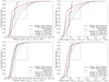 |
Fig. 1. Cumulative distribution of the binary masses (left) and the chirp masses (right). Top and bottom panels: results of the default and optimistic simulation setup, respectively. The solid red lines represent all formed double neutron star binaries in the simulation, which should be compared to the pulsar observations (solid black). The dashed black lines show the two reported merging events of neutron stars, which should be compared to the merging populations in the simulated data (dashed blue, dash dotted green, dash double-dotted purple). |
It is important to note that the pulsar population, observed in the Galactic disc, should be compared with all DNSs formed in the simulations, while the GW events should only resemble the simulated population, which merges at least within a Hubble time after star formation. The populations that merge faster tend to consist of more massive NSs, leading to a larger binary mass and chirp mass. While the default simulations better match the GW events (upper panels), the pulsar observations are better represented with the optimistic setup (lower panels). In both simulations, the merging DNS population contains fewer low-mass systems. The population merging within 0.1 Gyr after star formation contains the least less massive binaries. This can be seen in both mass distributions in Fig. 1 It should be noted that in both observational data sets, but especially for the GW events, the low number of observed systems may not represent the true population in the Universe.
3.2. Lower metallicity
At a lower metallicity, here close to that of the Large Magellanic Cloud (LMC, Z = 0.0047), DNS binaries seem to favour smaller masses (see Fig. 2). This even holds for the systems that merge fast enough to be observed as GW events. Here, it turns out that most systems formed with low mass would merge in such a low metallicity environment. This is mainly caused by the change in the envelope binding energy at lower metallicity.
It is important to be careful when comparing these results to the GW events as there is no information about the metallicity as long as there is no electromagnetic counterpart detected to identify the host galaxy. In the case of GW170817, the host galaxy has a metallicity comparable to that of the Milky Way, while in the case of GW190425 no host galaxy is identified. Furthermore, the different behaviour at lower metallicity requires more investigation in the future.
3.3. GW190425
The recently reported event GW190425 is likely to be a DNS merger, but the involvement of a black hole cannot be ruled out (Abbott et al. 2020; Kyutoku et al. 2020). The high mass of the system is thought to pose a problem for the formation of such a system and to be inconsistent with mass distribution of the known radio pulsars in the Milky Way (Abbott et al. 2020). Binary population synthesis calculations show that the formation of such a system at Milky Way-like metallicity is possible (see Fig. 3). Furthermore, the larger error bars compared to GW170817 provide weaker constrains to the binary and chirp mass, the best constrained masses of a GW event.
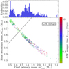 |
Fig. 3. Progenitor masses of GW190425 at Milky Way-like metallicity in the default simulation. The colour indicates the time until the GW merger. The models are selected according to the reported binary mass of |


The simulations cover progenitors with all kinds of merger delay times. There are two main populations. First, a population with the initially more massive star, here referred to as the primary, becoming an NS with a mass between 1.5 and 1.6 M⊙. In this case, the star with a lower zero-age main sequence mass gains mass during mass transfer episodes and finally becomes the more massive NS. This population prefers short delay times until merger. Second is a population with the primary’s mass mainly lying between 1.7 and 1.9 M⊙. Here, the primary is the more massive binary component. This population extends to masses of more than 2.1 M⊙. The more massive primaries prefer longer delay times, getting closer to the age of the Universe. The GW observations are incapable of differentiating between the two populations as these observations do not contain information about the formation order of the two NSs. A third, small population exceeds 2.3 M⊙ for the primary NS. In the simulations presented here, NS spin evolution is not followed. Abbott et al. (2020) predicted that the mass interval of the more massive component covers masses above 2.5 M⊙ for their high-spin prior. It is unclear whether such massive NSs exist (e.g. Özel & Freire 2016) and how they form.
The main formation channel for the GW190425 progenitors in the simulations contains a stable case B or case C mass transfer, in which the mass transfer initiates after the primary leaves the main sequence, onto its companion. After the primary explodes to form the first NS, the secondary evolves to fill its own Roche lobe. This leads to a CE phase, reducing the separation significantly. Before the CE, the binary needs a large separation in order to have the secondary star being evolved into a giant with a less tightly bound envelope when becoming the donor star. Only progenitor systems with longer delay times do not experience another mass transfer in terms of case BB, which is the mass transfer from a helium star after core helium exhaustion, leading to an ultra-stripped SN (Tauris et al. 2013). This formation channel including the case BB mass transfer is similar to the formation channel proposed by Romero-Shaw et al. (2020). In the default simulation the zero-age main sequence mass of the primary ranges from 16 to 30 M⊙, while the initial mass of the secondary is between 10 and 16 M⊙. The initial binary semi-major axis covers a range from 400 to 2000 R⊙, hence it is wide enough to initiate the first mass transfer only when the primary becomes a giant.
4. Discussions
At Milky Way metallicity, merging DNSs tend to have a larger binary and chirp mass than the entire formed DNS population. The set of DNSs, which is only part of the formed but not merging population, contains the systems that have a large separation. Those binaries require smaller kicks from the SN in order to remain bound. Electron-capture SNe are expected to have smaller kicks, as they eject less material. Thus, NSs formed in an electron-capture SN can more easily create wider DNSs. As the merging population did not include those systems, the relative abundance of more massive DNSs is larger for this population. This coincides with the fact that many DNSs from radio pulsar observations in the Milky Way have long merger delay times and would not merge within a Hubble time via GW radiation (Tauris et al. 2017). It should be noted that there is still a mass discrepancy between the most common population in the simulation, mainly formed via electron-capture SNe, and the pulsar observations (Kruckow et al. 2018). Beside this small mass discrepancy, the population from the optimistic simulation is similar to the distribution found in Farrow et al. (2019). The only other difference is that here the most massive DNSs are a bit more massive. Another possibility of enriching the massive binary content of the merging population is a dynamical tightening in star clusters (e.g. Ye et al. 2020).
The situation at lower metallicity differs from the simulations at Milky Way-like metallicity (cf. Figs. 1 and 2). The simulations at lower metallicity should be taken with a grain of salt as there are no strong constrains provided by observations of binaries containing NSs at lower metallicity and/or outside the Milky Way. There are no radio pulsar observations of DNSs or detailed observations of X-ray binaries as progenitors of those. Hence, the populations in the Milky Way and other galaxies may differ for other reasons (Pankow 2018).
The progenitor of GW190425 (see Fig. 3) shows possible component masses up to 2.3 M⊙, which is consistent with the recent results of Woosley et al. (2020) for NS masses from helium stars at solar metallicity. Other investigations of double neutron star mergers (e.g. Mapelli et al. 2019) suggest individual component masses are just below 2.0 M⊙. Masses up to 2.7 M⊙, as suggested by the high-spin analysis of GW190425 (Abbott et al. 2020), are not obtained by calculations of binary evolution. This may indicate a less massive fast spinning or a slow spinning NS as the more massive component in the merging event. Furthermore, a possible black hole origin cannot be ruled out. However, it should be noted that such a less massive black hole would challenge isolated binary evolution as well.
5. Conclusions
Using the default setup, the DNS population merging within 0.1 Gyr coincides well with GW170817 and GW190425. If these two events are representative of further GW detections of merging DNS, they match the simulations. At the same time, the simulations produce less massive systems in wider orbits. Those are more consistent with the radio pulsar population observed in the Milky Way. Because of the low number of observations, the mass distribution of merging DNSs is not finalised yet. However, it cannot be concluded that the pulsar population and the DNS merger population are not consistent.
The recently reported event GW190425 has possible progenitors from the current understanding of binary evolution. Depending on the detailed component masses, the delay time of the merger differs significantly. The simulations cannot reproduce the high-spin models with a very high-mass component. Due to its host galaxy having not been identified, no information about the metallicity of the progenitor and its possible delay time since star formation can be used to further narrow the mass estimate of the event.
Acknowledgments
I would like to thank Hailiang Chen and Yan Gao for some feedback to this paper. This work is partly supported by Grant No. 11521303 and 11733008 of the Natural Science Foundation of China.
References
- Abbott, B. P., Abbott, R., Abbott, T. D., et al. 2017, Phys. Rev. Lett., 119, 161101 [NASA ADS] [CrossRef] [PubMed] [Google Scholar]
- Abbott, B. P., Abbott, R., Abbott, T. D., et al. 2020, ApJ, 892, L3 [Google Scholar]
- Abt, H. A. 1983, ARA&A, 21, 343 [Google Scholar]
- Andrews, J. J., & Mandel, I. 2019, ApJ, 880, L8 [CrossRef] [Google Scholar]
- Cameron, A. D., Champion, D. J., Kramer, M., et al. 2018, MNRAS, 475, L57 [CrossRef] [Google Scholar]
- Champion, D. J., Lorimer, D. R., McLaughlin, M. A., et al. 2004, MNRAS, 350, L61 [NASA ADS] [CrossRef] [Google Scholar]
- Chattopadhyay, D., Stevenson, S., Hurley, J. R., Rossi, L. J., & Flynn, C. 2020, MNRAS, 494, 1587 [CrossRef] [Google Scholar]
- Corongiu, A., Kramer, M., Stappers, B. W., et al. 2007, A&A, 462, 703 [NASA ADS] [CrossRef] [EDP Sciences] [Google Scholar]
- de Kool, M. 1990, ApJ, 358, 189 [NASA ADS] [CrossRef] [Google Scholar]
- Farrow, N., Zhu, X.-J., & Thrane, E. 2019, ApJ, 876, 18 [CrossRef] [Google Scholar]
- Ferdman, R. D., Stairs, I. H., Kramer, M., et al. 2014, MNRAS, 443, 2183 [CrossRef] [Google Scholar]
- Fonseca, E., Stairs, I. H., & Thorsett, S. E. 2014, ApJ, 787, 82 [CrossRef] [Google Scholar]
- Kramer, M., Stairs, I. H., Manchester, R. N., et al. 2006, Science, 314, 97 [NASA ADS] [CrossRef] [PubMed] [Google Scholar]
- Kroupa, P. 2008, in The Cambridge N-Body Lectures, eds. S. J. Aarseth, C. A. Tout, & R. A. Mardling (Berlin Springer Verlag), Lect. Notes Phys., 760, 181 [NASA ADS] [CrossRef] [Google Scholar]
- Kruckow, M. U., Tauris, T. M., Langer, N., Kramer, M., & Izzard, R. G. 2018, MNRAS, 481, 1908 [NASA ADS] [CrossRef] [Google Scholar]
- Kuiper, G. P. 1935, PASP, 47, 15 [NASA ADS] [CrossRef] [Google Scholar]
- Kyutoku, K., Fujibayashi, S., Hayashi, K., et al. 2020, ApJ, 890, L4 [CrossRef] [Google Scholar]
- Lynch, R. S., Swiggum, J. K., Kondratiev, V. I., et al. 2018, ApJ, 859, 93 [NASA ADS] [CrossRef] [Google Scholar]
- Mapelli, M., Giacobbo, N., Santoliquido, F., & Artale, M. C. 2019, MNRAS, 487, 2 [NASA ADS] [CrossRef] [Google Scholar]
- Martinez, J. G., Stovall, K., Freire, P. C. C., et al. 2015, ApJ, 812, 143 [NASA ADS] [CrossRef] [Google Scholar]
- Martinez, J. G., Stovall, K., Freire, P. C. C., et al. 2017, ApJ, 851, L29 [CrossRef] [Google Scholar]
- Moriya, T. J., Mazzali, P. A., Tominaga, N., et al. 2017, MNRAS, 466, 2085 [NASA ADS] [CrossRef] [Google Scholar]
- Öpik, E. 1924, Pub. Tartu Astrofizica Observ., 25 [Google Scholar]
- Özel, F., & Freire, P. 2016, ARA&A, 54, 401 [Google Scholar]
- Pankow, C. 2018, ApJ, 866, 60 [CrossRef] [Google Scholar]
- PALFA Collaboration (Ferdman, R. D., et al.) 2018, in Pulsar Astrophysics the Next Fifty Years, eds. P. Weltevrede, B. B. P. Perera, L. L. Preston, et al., IAU Symp., 337, 146 [Google Scholar]
- Peters, P. C. 1964, Phys. Rev., 136, 1224 [Google Scholar]
- Romero-Shaw, I. M., Farrow, N., Stevenson, S., Thrane, E., & Zhu, X. J. 2020, MNRAS, 496, L64 [CrossRef] [Google Scholar]
- Salpeter, E. E. 1955, ApJ, 121, 161 [Google Scholar]
- Scalo, J. M. 1986, Fund. Cosmic Phys., 11, 1 [NASA ADS] [EDP Sciences] [Google Scholar]
- Soberman, G. E., Phinney, E. S., & van den Heuvel, E. P. J. 1997, A&A, 327, 620 [NASA ADS] [Google Scholar]
- Stovall, K., Freire, P. C. C., Chatterjee, S., et al. 2018, ApJ, 854, L22 [CrossRef] [Google Scholar]
- Suwa, Y., Yoshida, T., Shibata, M., Umeda, H., & Takahashi, K. 2015, MNRAS, 454, 3073 [CrossRef] [Google Scholar]
- Swiggum, J. K., Rosen, R., McLaughlin, M. A., et al. 2015, ApJ, 805, 156 [CrossRef] [Google Scholar]
- Tauris, T. M., & Takens, R. J. 1998, A&A, 330, 1047 [NASA ADS] [Google Scholar]
- Tauris, T. M., Langer, N., Moriya, T. J., et al. 2013, ApJ, 778, L23 [NASA ADS] [CrossRef] [Google Scholar]
- Tauris, T. M., Langer, N., & Podsiadlowski, P. 2015, MNRAS, 451, 2123 [NASA ADS] [CrossRef] [Google Scholar]
- Tauris, T. M., Kramer, M., Freire, P. C. C., et al. 2017, ApJ, 846, 170 [NASA ADS] [CrossRef] [Google Scholar]
- van Leeuwen, J., Kasian, L., Stairs, I. H., et al. 2015, ApJ, 798, 118 [NASA ADS] [CrossRef] [Google Scholar]
- Vigna-Gómez, A., Neijssel, C. J., Stevenson, S., et al. 2018, MNRAS, 481, 4009 [NASA ADS] [CrossRef] [Google Scholar]
- Webbink, R. F. 1984, ApJ, 277, 355 [NASA ADS] [CrossRef] [Google Scholar]
- Weisberg, J. M., Nice, D. J., & Taylor, J. H. 2010, ApJ, 722, 1030 [NASA ADS] [CrossRef] [Google Scholar]
- Woosley, S., Sukhbold, T., & Janka, H. T. 2020, ApJ, 896, 56 [CrossRef] [Google Scholar]
- Ye, C. S., Fong, W.-F., Kremer, K., et al. 2020, ApJ, 888, L10 [CrossRef] [Google Scholar]
Appendix A: Observational data
Information about DNSs are obtained from pulsar observation in the Milky Way and inferred from GW merging events. All the observational data on the masses of DNS can be found in Table A.1. The chirp masses for the DNSs in the Milky Way are calculated from the individual masses in the ten cases, where this data is available.
The pulsar observations are limited to the Milky Way, while the GW observations lack precise sky localisation. The pulsar observations are incomplete for binaries with very long orbital periods (>1 yr). Additionally, the discoveries of pulsars in a binary is more likely for systems with lower acceleration, hence not eccentric and/or not too tight. On the other hand, the GW observations provide no information about the local environment of an event as long as no electromagnetic counterpart is identified. The GW events with larger masses have a larger GW amplitude, which helps to identify them close to the detection limit.
First table: summary of the GW events. Second table: pulsar observations.
All Tables
Initial values and settings of key input physics parameters for the default and optimistic simulation, taken from Tables 2 and 8 of Kruckow et al. (2018).
All Figures
|
Fig. 1. Cumulative distribution of the binary masses (left) and the chirp masses (right). Top and bottom panels: results of the default and optimistic simulation setup, respectively. The solid red lines represent all formed double neutron star binaries in the simulation, which should be compared to the pulsar observations (solid black). The dashed black lines show the two reported merging events of neutron stars, which should be compared to the merging populations in the simulated data (dashed blue, dash dotted green, dash double-dotted purple). |
| In the text | |
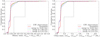 |
Fig. 2. Similar to the upper panels of Fig. 1 but for lower metallicity. |
| In the text | |
|
Fig. 3. Progenitor masses of GW190425 at Milky Way-like metallicity in the default simulation. The colour indicates the time until the GW merger. The models are selected according to the reported binary mass of |
| In the text | |
Current usage metrics show cumulative count of Article Views (full-text article views including HTML views, PDF and ePub downloads, according to the available data) and Abstracts Views on Vision4Press platform.
Data correspond to usage on the plateform after 2015. The current usage metrics is available 48-96 hours after online publication and is updated daily on week days.
Initial download of the metrics may take a while.