| Issue |
A&A
Volume 639, July 2020
|
|
|---|---|---|
| Article Number | A3 | |
| Number of page(s) | 13 | |
| Section | Planets and planetary systems | |
| DOI | https://doi.org/10.1051/0004-6361/201937267 | |
| Published online | 01 July 2020 | |
Aluminium oxide in the atmosphere of hot Jupiter WASP-43b
1
SRON Netherlands Institute for Space Research,
Sorbonnelaan 2,
3584
CA,
Utrecht, The Netherlands
e-mail: This email address is being protected from spambots. You need JavaScript enabled to view it.
2
Centre for Exoplanet Science, University of St Andrews,
Nort Haugh,
St Andrews,
KY169SS,
UK
3
Department of Physics and Astronomy, University College London,
London,
WC1E 6BT,
UK
Received:
5
December
2019
Accepted:
7
April
2020
Abstract
We have conducted a re-analysis of publicly available Hubble Space Telescope Wide Field Camera 3 (HST WFC3) transmission data for the hot-Jupiter exoplanet WASP-43b, using the Bayesian retrieval package Tau-REx. We report evidence of AlO in transmission to a high level of statistical significance (>5σ in comparison to a flat model, and 3.4σ in comparison to a model with H2O only). We find no evidence of the presence of CO, CO2, or CH4 based on the available HST WFC3 data or on Spitzer IRAC data. We demonstrate that AlO is the molecule that fits the data to the highest level of confidence out of all molecules for which high-temperature opacity data currently exists in the infrared region covered by the HST WFC3 instrument, and that the subsequent inclusion of Spitzer IRAC data points in our retrieval further supports the presence of AlO. H2O is the only other molecule we find to be statistically significant in this region. AlO is not expected from the equilibrium chemistry at the temperatures and pressures of the atmospheric layer that is being probed by the observed data. Its presence therefore implies direct evidence of some disequilibrium processes with links to atmospheric dynamics. Implications for future study using instruments such as the James Webb Space Telescope are discussed, along with future opacity needs. Comparisons are made with previous studies into WASP-43b.
Key words: planets and satellites: atmospheres / infrared: planetary systems / planets and satellites: gaseous planets / molecular data
© ESO 2020
1 Introduction
WASP-43b has been the subject of many scientific studies in recent years (e.g. Mendonça et al. 2018a; Louden & Kreidberg 2018; Gandhi & Madhusudhan 2017; Komacek et al. 2017; Keating & Cowan 2017; Kataria et al. 2015), largely because it is one of only a few exoplanets to have observed emission phase curve data (Stevenson et al. 2014) with strong evidence of molecular signatures, as demonstrated by Kreidberg et al. (2014). The planet is assumed to be tidally locked, which means that some information on atmospheric variability across the planet’s surface can be gained via analysis of this emission data at different phases of planetary transit, making it a strong candidate for detailed studies of atmospheric circulation models. It was discovered by Hellier et al. (2011) around an active K7V star, with deduced planetary parameters from radial velocity measurements and transit observations of 2.034 ± 0.052 MJ and 1.036 ± 0.019 RJ (Gillon et al. 2012). The presence of strong equatorial jets has been suggested by previous studies, such as Kataria et al. (2015), largely due to the strong day–night temperature contrast (Stevenson et al. 2014; Kataria et al. 2015; Gandhi & Madhusudhan 2017; Irwin et al. 2020) to explain the eastward hotspot shift of 12.3 ± 1° (corresponding to 40 min before the eclipse) observed by Stevenson et al. (2014).
The publicly available transmission and emission data for WASP-43b is primarily a result of observations by the Wide Field Camera 3 (WFC3) instrument on the Hubble Space Telescope (HST). WFC3 was used to observe three full-orbit phase curves, three primary transits, and two secondary eclipses (proposal ID 13467, PI: Jacob Bean; Bean 2013). The first light-curve fitting of the transmission data was carried out by Kreidberg et al. (2014), and later independently by Tsiaras et al. (2018). We consider both sets of data in this work. Spitzer IRAC data measured at 3.6 μm and 4.5 μm is available from Blecic et al. (2014), with an independent re-analysis of the transit depth from Morello et al. (2019). Previous analyses of the WFC3 data by Kreidberg et al. (2014) and Stevenson et al. (2017) have found evidence of H2O in both transmission and emission, with Stevenson et al. (2017) deducing the presence of CO and/or CO2 based on the Spitzer data points. Weaver et al. (2020) also find evidence of H2O in transmission. CH4 was found to vary in emission with phase by Stevenson et al. (2017), with some caution on the derived abundances demonstrated by Feng et al. (2016).
AlO has been detected in oxygen-rich stars (e.g. De Beck et al. 2017; Takigawa et al. 2017). There has, however, only been one previous observed indication of AlO in an exoplanet atmosphere, by von Essen et al. (2019) in the atmosphere of the highly irradiated “super-hot Jupiter” WASP-33b. They speculate about the presence of a thermalinversion; Gandhi & Madhusudhan (2019) have also recently proposed AlO as a species that could cause a thermal inversion. As well as giving insight into the atmosphere, detecting heavy elements such as Al in a planetary atmosphere also gives some insight into planet formation processes (Johnson & Li 2012; Hasegawa & Hirashita 2014).
Although not explicitly stated, it is assumed that the study of von Essen et al. (2019) uses the line list for AlO by Patrascu et al. (2015), which was computed in 2015 as part of the ExoMol project (Tennyson et al. 2016)and remains the only high-temperature line list for AlO suitable for retrievals of this kind. The line list is valid up to 8000 K, includes various electronic states (Patrascu et al. 2014), covers the region 0.28–100 μm, and consistsof over 5 million transitions, making it highly suitable for the characterisation of exoplanet or stellar atmospheres. The studies of De Beck et al. (2017) and Takigawa et al. (2017), on the other hand, rely on a handful of individual lines from rotational transitions and, although the source of their opacity data is again not explicitly stated, it is assumed that experimental data was used.
This paper is structured as follows. In Sect. 2, we provide details of our retrieval process and the statistical measures used, followed by the results in Sect. 3. We discuss various aspects of the results in Sect. 4, including the presence of clouds in Sect. 4.1, and equilibrium chemistry in Sect. 4.2. In Sect. 4.3 we discuss the effects of including available transmission spectra from other instruments in different wavelength regions, which is followed by a comment on the currently available opacity data in Sect. 4.4. Our summary is given in Sect. 5.
Free parameters used in the TauREx retrievals.
2 Methods
2.1 Transmission retrieval
For the retrievals presented in this work, we use the Bayesian retrieval package Tau-REx (Waldmann et al. 2015). Some preliminary tests and checks were conducted independently using Bayesian retrieval package ARCiS (Min et al. 2020). Both codes use the multinest (Feroz & Hobson 2008; Feroz et al. 2009, 2013) algorithm to sample the specified parameter space for the region of maximum likelihood. Of these two codes, only Tau-REx is currently publicly available. Full details on the ARCiS code are presented in a separate paper (Min et al. 2020). The most important information can be found in Ormel & Min (2019). The code consists of a forward modelling part based on correlated-k molecular opacities and cloud opacities using Mie and distribution of hollow spheres (DHS; see Min et al. 2005) computations. With ARCiS it is possible to compute cloud formation (Ormel & Min 2019) and chemistry (Woitke et al. 2018) from physical and chemical principles. The code has been benchmarked against petitCODE (Mollière et al. 2015) in Ormel & Min (2019). For the retrieval part the multinest algorithm is employed. Benchmarks for the retrieval have been performed in the framework of the ARIEL mission (Pascale et al. 2018) showing excellent agreement with multiple other retrieval codes.
We have recently converted all molecular line list data available from the ExoMol (Tennyson et al. 2016) and HITEMP (Rothman et al. 2010) databases into cross sections and k-tables, for input into both Tau-REx and ARCiS. Cross sections and k-tables were computed at R =  = 10 000 and R = 300, respectively, on a grid of 27 temperatures between 100 and 3400 K, and 22 pressures between 1×10⁻⁵ and 100 bar. Details of the parameters and file formats used for these opacity data, which were converted into cross sections using ExoCross (Yurchenko et al. 2018a), are outlined in Chubb et al. (2020a), along with the publicly available opacities.
In order to fully assess which of these molecules is most likely to be causing the absorption features observed in the transmission spectrum of WASP-43b, we carried out the following steps, going from simple to more complex retrieval procedures:
- 1.
We first carried out a set of simple free retrievals that each include only one molecule, in order to subsequently exclude those with no absorption features in the WFC3 HST wavelength region (1.1–1.7 μm).
- 2.
Forward models for individual species, computed using ARCiS, are given in Fig. B.1, plotted alongside the transmission data for WASP-43b from Kreidberg et al. (2014). These were used in order to help assess which molecules to include in subsequent retrievals. These figures are intended to give an indication of where absorption features would occur in the HST WFC3 region for each of these species, and are not the results of the free retrievals specified in step 1.
- 3.
We then assessed the reduced χ2 value for another set of simple retrievals, which each include only two molecules: H2O plus one other molecule. For this we consider all the molecules that were found to exhibit some absorption features in the WFC3 HST wavelength region, as determined in steps 1 and 2. ARCiS was used for steps 1–3.
- 4.
We set up more complex retrievals using Tau-REx, the results of which are presented in Sect. 3. Much of the set-up for these retrievals are as described in Tsiaras et al. (2018), with a summary of the free and fixed parameters used in the present work given in Tables 1 and 2, respectively. We used free retrievals here with regard to the molecular abundances; i.e. no chemistry was assumed, and the volume mixing ratio for each molecular or atomic species was allowed to vary within the bounds specified by Table 1.
Fixed parameters used in the TauREx retrievals.
2.2 Statistical measures
In order to assess which molecule, or combination of molecules, is most likely to be causing the absorption features observed in WASP-43b, we use the following statistical measures.
For step 3 of Sect. 2.1, the reduced χ2 value is used as part of the assessment to determine which molecules to include in subsequent retrievals. The reduced χ2 is a simple metric used to determine how well a particular model (in this case the results of our retrieval) fits a set of observed data. The use of reduced χ2, as opposed to χ2, means that retrievals using different number of molecular absorbers can be directly compared. The data we use here is the transmission spectra of WASP-43b from the HST WFC3 instrument, as analysed and presented in Kreidberg et al. (2014). A smaller reduced χ2 generally indicates a retrieval result that fits the observed data better, with a value <1 usually being an indication of over-fitting. Formally, models with a reduced χ2 closest to 1 are favoured over other models. However, we show through further assessments that this is not the case for, for example, the C2 H2 + H2O model. This model has a reduced χ2 close to 1, but the inclusion of C2 H2 is found not to be significant when considering the Bayes factors of various models (see discussion above and Sect. 3). We conclude that the use of reduced χ2 as a guide is limited and prone to error, and therefore a more rigorous approach is required. For this reason, we conduct the following Bayesian analysis for the full set of molecules used for this reduced χ2 assessment (see Sect. 3 and Tables 3 and A.1).
For step 4 of Sect. 2.1, we use a more rigorous way to determine the likelihood of a retrieval in comparison to the prior base set-up: the Nested Sampling Global Log-Evidence (log(E)). This is given as an output from the Multinest algorithm (Feroz & Hobson 2008; Feroz et al. 2009, 2013). This Bayesian log-evidence is then used to find the Bayes Factor (B01) (see e.g. Waldmann et al. 2015), which is a measure to assess the significance of one model against another (here “model” refers to the set of free parameters used, in particular which molecular absorbers and whether clouds are included). If the natural log of the Bayes Factor, ln(B01) > 5 then, according to Trotta (2008), the model can be considered significant with respect to the base model; ln(B01) > 5 corresponds to >3.6σ detection over the base model, while ln(B01) > 11 corresponds to >5σ detection over the base model.
3 Retrieval results
The reduced χ2 values found in step 2 of Sect. 2.1 are given in Table 3, along with the line list data used for each molecule. AlO and H2O were among the molecules with the smallest reduced χ2. It should be noted that the value of reduced χ2 itself is not exact and is prone to error, and so is only used here as a guide to which molecules to include in subsequent retrievals. The models with χ2 < 1 (usually an indicator of over-fitting) cannot be distinguished from one another.
The full retrievals that were outlined in step 3 of Sect. 2.1, were performed using Tau-REx (see Tables 1 and 2 for the free and fixed parameters used, respectively). Table 4 gives a summary of the Nested Sampling Global Log-Evidence (see Sect. 2.2) of various retrievals, along with the natural log of the Bayes factor, ln(B01), and σ likelihood against: a flat base retrieval (i.e. one with no molecular features), a retrieval with only H2O included, and a retrieval with only AlO included. Here the transmission spectra of WASP-43b from the HST WFC3 instrument is used, as analysed and presented in Kreidberg et al. (2014).
It can be seen that the best model against a flat spectra is that where both AlO and H2O are included in the retrieval, which is preferred over a flat-line base model at over 5σ. The findings of Table 4 show that the presence of AlO in the model gives more of a statistical improvement to the fit than the inclusion of H2O; a model with both H2O and AlO is preferred over a model with only H2O at a confidence level of 3.4σ, whereas a model with H2O and AlO is preferred over a model with only AlO at a confidence level of 2.6σ. Table A.1 gives ln(B01) for H2O + each molecule which is considered in Table 3. The line list sources are given in Table 3. In all these models we include Rayleigh scattering and collision induced absorption (CIA) of H2 –He and H2 –H2 (Gordon et al. 2017; Borysow et al. 2001). In order to check whether the inclusion of these continuum opacities has a significant effect on our results, we performed a series of retrievals with and without their inclusion. It can be seen from Table A.2 that although there is some small variation in the Nested Sampling Global Log-Evidence for different combinations of including or not including CIA, Rayleigh scattering and clouds (for models with H2O only and with H2O + AlO), we find that the inclusion of CIA and Rayleigh scattering does not significantly affect the results, and that the H2O + AlO model is preferred over the H2O-only model for all combinations.
Figure 1 shows the results of a retrieval which includes AlO and H2O (top panel) and a retrieval only including H2O (bottom panel). Figure 2 illustrates the contributions of molecular features in the former. The posterior distributions of this cloud-free model with AlO and H2O only are given in Fig. 3. For comparison, we ran the same models using the outputs (based on the same observations) of the transit light-curve fitting by Tsiaras et al. (2018). Although the Nested Sampling Global Log-Evidence was higher in all cases for the Tsiaras et al. (2018) data (most likely due to the higher number of derived data points), the Bayes factor was consistent with those presented in Table 4. We only include those models with the highest Bayes factors here;the inclusion of other molecules consistently gave negative (or <1) Bayes factors in comparison to the H2O + AlO model, indicating that their inclusion is not statistically favoured (see Table A.1 for the full list). The only exception here is that a model with H2O + AlO + Na gave aweak-to-moderate detection of Na when using the high-res data from Tsiaras et al. (2018) (a Bayes factor of 2.2, corresponding to ~2.6σ, in comparison to the same model with Na discluded). The same finding does not apply when using the data from Kreidberg et al. (2014); the far left data point on the former is not included in the latter, presumably due to concerns about the reliability of data fromthe edges of the WFC3 wavelength window. We therefore do not find any strong justification to include Na in our models. We also tried various retrievals with and without clouds, and found no strong evidence to justify including clouds in our model; the inclusion of clouds resulted in a negative Bayes factor, which demonstrates that the inclusion of extra parameters is not justified (based on the present data quality and number of observed data points) by a corresponding improvement in the fit.
Reduced χ2 for different combinations of molecules (in addition to H2O) included in a cloud-free retrieval using ARCiS, and references for the line lists used.
Nested sampling global log-evidence (log(E)) of various retrievals of the HST/WFC3 data, along with the natural log of the Bayes factor, ln(B01), and σ likelihood against: a flat “base” retrieval (i.e. with no molecular features), a retrieval with only H2O included, and a retrieval with only AlO included.
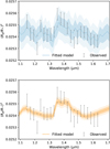 |
Fig. 1 Cloud-free Tau-REx transmission retrieval results with H2O and AlO (top) and with H2O only (bottom). The different shading corresponds to 1σ and 2σ regions. |
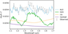 |
Fig. 2 Contributions of molecular features to the cloud-free Tau-REx retrieval results that include AlO and H2O only. |
4 Results
No other molecules apart from H2O and AlO were found to be statistically significant from our retrievals of the HST WFC3 data (or from the inclusion of Spitzer IRAC data) for WASP-43b. This is most likely either because other molecular species that are present do not have strong absorption features in the region of the WFC3 data or because they do but they are present in an abundance too low to be strongly detectable. It should be noted that the WFC3 transmission data is only probing a small layer in the upper atmosphere at the terminator regions of the planet, mainly in the region of 10−3–10−1 bar. In this section we discuss various aspects of our findings.
4.1 Clouds
Although we did not find any statistical reason to include clouds in these retrievals, it is of interest to explore further the presence and type of clouds present on WASP-43b, as is done in Helling et al. (2020). It is possible that there are clouds, but they are either lower in the atmosphere, they do not cover the whole planetary surface, or they are so thin as to appear transparent. The models of Parmentier et al. (2016) suggest that clouds are expected to always be present on the nightside of hot Jupiters, and previous studies such as Mendonça et al. (2018b) and Komacek et al. (2017) indicate that there is a thick cloud layer on the nightside of WASP-43b. Works such as Venot et al. (2020) point out the difficulty in differentiating between a cloudy and cloud-free model by retrieving HST/WFC3 data alone. Their models suggest the nightside of WASP-43b is cloudy, and the cloud coverage of the dayside depends on various microphysical processes and dynamics.
Cloud formation in giant gas planets occurs from a chemically very rich atmospheric gas causing the formation of cloud particles that are made of a whole mix of materials, including Mg/Si/Fe/O-solids and also high-temperature condensates like TiO2[s] and Al2 O3[s], e.g. in HD 189733 b and HD 209458 b (Helling et al. 2016). The amount by which these cloud particles deplete the local element abundance depends on the local thermodynamic properties of the atmosphere, which in turn determines the gas composition, and hence the abundance of gas species such as AlO. A variety of cloud species are thought likely to be present in the atmosphere of WASP-43b, including corundum, Al2 O3[s] (Helling et al. 2020). More detailed studies are required to determine in detail the interplay between local thermodynamics and cloud formation which would allow the presence of AlO in sufficient amounts to explain the findings of this work.
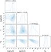 |
Fig. 3 TauRex transmission retrieval posteriors for H2O and AlO, with no clouds. |
4.2 Chemistry
There are a few aluminium hosting molecules that equilibrium chemistry models such as GGchem (Woitke et al. 2018) predict are more abundant than AlO at the temperatures and pressures expected in the region of the atmosphere being probed by the WFC3 transmission spectrum of WASP-43b, if solar elemental abundances are assumed. The most notable of these molecules are AlH, AlCl, AlF, Al2O, AlOH, and atomic Al (which does not become Al+ until higher temperatures, around 3000 K). These would all ideally be included in further retrievals for the transmission spectra of WASP-43b. The availability of opacity data for these and other molecules will be discussed in Sect. 4.4.
The presence of AlO in the region of the atmosphere we are probing (at the terminator regions, around 10−3–10−1 bar, i.e. relatively high in the atmosphere) is an indication of some disequilibrium processes at work in the atmosphere of WASP-43b; there has been speculation about such processes in the atmospheres of hot-Jupiter exoplanets similar to WASP-43b (see e.g. Stevenson et al. 2010). Although we do not know the exact cause of the disequilibrium processes at work in WASP-43b, the presence of AlO is most likely due to either vertical or horizontal mixing; equilibrium chemistry models predict AlO to be present at high abundance deeper in the atmosphere than the relatively high-up layers being probed by HST WFC3, and aluminium-bearing cloud species such as Al2O3[s] are expected to be present across the planet’s atmosphere (Helling et al. 2020). It is therefore either possible for turbulence to be dredging up gases towards the top of the atmosphere, and therefore causing the apparent deviation from equilibrium chemistry, or for the evaporation of clouds to be creating AlO gas in the hottest parts of the atmosphere, which could be horizontally transported to the terminator regions we are observing by the strong equatorial jets which have been suggested by previous studies, such as Kataria et al. (2015). It has also been shown by Agúndez et al. (2014) that, for hot Jupiters similar to WASP-43b, horizontal mixing causes the volume mixing ratio of molecules at the terminator regions to become quenched towards values typical of the hottest dayside region. More detailed studies, however, are required to determine in detail the interplay between local thermodynamics and cloud formation which would allow the presence of AlO in sufficient amounts to explain the findings of this work. Although, as mentioned above, the dominant Al-binding species in equilibrium is AlOH, relatively little is known about the kinetic and photochemistry of such metal binding species. It has been demonstrated the AlO plays a key role in forming clusters such as (Al2 O3)n in AGB staroutflows (Boulangier et al. 2019), and that AlO has been identified in the cold envelopes of AGB star R Dor based on kinetic gas-phase simulations (Decin et al. 2017). It is therefore possible that AlO in an exoplanet atmosphere could be a indicator of kinetic chemistry, which affects metal-containing species. We thus plan to assess the potential effect of mixing for WASP-43b in future work, combined with more detailed cloud formation models, in order to assess the validity of various disequilibrium processes.
The asymmetry of the phase curve emission data for WASP-43b suggests some variation in molecular signatures across the planetary surface (Stevenson et al. 2017), as has been recently demonstrated for HAT-P-7b (Helling et al. 2019). It should be noted that this planet is considerably more irradiated than WASP-43b. More investigation is needed to determine whether AlO is observed in emission and in transmission, which, due to available emission phase spectroscopic data for WASP-43b, would give further insight into the varying abundances of different gases throughout different latitudes and altitudes of the planetary atmosphere.
4.3 Spitzer and other observational data
As mentioned above, Spitzer data measured at 3.6 and 4.5 μm are available from Blecic et al. (2014), with an independent re-analysis of the transit depth from Morello et al. (2019). We did not include these points in the initial retrieval due to large variation in their deduced transit depths depending on the method used to fit the data (see e.g. Morello et al. 2019). The dip at 3.6 microns and increased absorption at 4.5 microns was found by Kreidberg et al. (2014) to be consistent with either CO or CO2. It should be noted that this dip is less pronounced with the Spitzer data analysed by Morello et al. (2019). Other molecules that exhibit a similar dip at 3.6 μm and increased absorption at 4.5 μm include SiO (Barton et al. 2013), AlF (Yousefi & Bernath 2018), CaF (Hou & Bernath 2018), LiCl (Bittner & Bernath 2018), NS (Yurchenko et al. 2018b), PO, and PS (Prajapat et al. 2017). The current data availability for these molecules is discussed in Sect. 4.4.
We ran some retrievals including the Spitzer points of Blecic et al. (2014). Figure 4 shows the resulting cloud-free retrieval and molecular contributions for AlO and H2O only. Figure 5 shows the resulting cloud-free retrieval and molecular contributions for CO2 and H2O only. The model with H2O and AlO is very strongly preferred over that with H2O and CO2; it gives a Bayes Factor of 12.4, corresponding to a significance of higher than 5σ. A model with H2O and AlO gives a similar Bayes factor of 12.0 when compared to one with H2O only. We tried all the molecules mentioned above and did not find any evidence to include any of them. We arrive at the same conclusion when using the Spitzer points from Morello et al. (2019), and when replacing CO2 with CO (Li et al. 2015).
Some ground-based observations of WASP-43b have also been made, with available data in the optical region from ground-based instruments from Murgas et al. (2014) and Weaver et al. (2020), and broad-band data from Chen et al. (2014) and Valyavin et al. (2018); we also did not use them for our retrievals, due to their large uncertainties and issues with combining data from different instruments. The most notable AlO absorption feature can be seen in the top panel of Fig. 6, at around 0.4–0.5 μm. More accurate observations in this region would help confirm our findings and constrain AlO abundances. Evidence was found by Murgas et al. (2014) for the Na I doublet around 589 nm at around 2.9σ confidence, but no evidence of K. Weaver et al. (2020) recently found no evidence of either Na or K. The data of both studies do not cover the region of AlO absorption at around 0.4–0.5 μm.
Figure 6 illustrates some absorption features in the wavelength region of James Webb Space Telescope (JWST) (0.6–28 μm) and ARIEL (0.5–7.8 μm), which could help confirm our detections and constrain the molecular abundances and other retrieved parameters, which we note cannot be constrained by WFC3 data alone. For simplicity, we compare best fit forward models, based on retrievals using H2O only, AlO only, H2O + AlO, and H2O only, H2O + CO2, H2O + CO2 + AlO. Unfortunately, one of the most prominent absorption features of AlO occurs just below 0.5 μm (see the top panel of Fig. 6), which would therefore not be observable by either JWST or ARIEL. The Twinkle space telescope, however, which is due for launch in early 2022, has two spectrometers (visible, 0.4–1 μm, and infrared, 1.3–4.5 μm) (Edwards et al. 2019), and so should be able to observe this feature. The Hubble STIS instrument is currently available, with an observational wavelength region which also covers that of the strong AlO absorption feature.
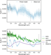 |
Fig. 4 Tau-REx transmission retrieval results, including Spitzer points from Blecic et al. (2014), with H2O and AlO (top) and the contributions of each molecule to the retrieval result (bottom). The different shading in the first panel corresponds to 1σ and 2σ regions. |
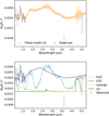 |
Fig. 5 Tau-REx transmission retrieval results, including Spitzer points from Blecic et al. (2014), with H2O and CO2 (top) and the contributions of each molecule to the retrieval result (bottom). The different shading in the first panel corresponds to 1σ and 2σ regions. |
4.4 Opacity data requirements
Of the above-mentioned Al-containing species that are expected from chemical equilibrium processes (see Sect. 4.2), opacity line list data in the IR region covered by HST and Spitzer data exist for AlH (Yurchenko et al. 2018c) and AlO (Patrascu et al. 2015) only. There are no significant absorption features in the 1.1–1.7 μm region for AlH, but there is some absorption in the region where the Spitzer data covers, around 3.6 μm. There is data available from MoLLIST (Bernath 2020), which can be found in ExoMol format (Wang et al. 2020) on the ExoMol website, for AlF and AlCl (Yousefi & Bernath 2018). This data, however, only extends up to around 2350 cm−1 for AlCl and 3900 cm−1 for AlF (i.e. it does not cover below 4.2 or 2.5 μm for AlCl and AlF, respectively). There is currently no line list data available in the literature for Al2 O or AlOH.
Regarding the species mentioned in Sect. 4.3, which could potentially be used to explain the Spitzer data points, the line list data for SiO (Barton et al. 2013), AlF (Yousefi & Bernath 2018), and CaF (Hou & Bernath 2018) are currently not computed up to a high enough energy (relating to a low enough wavelength) to cover the region of the WFC3 data, or into the visible. The line list data for NS (Yurchenko et al. 2018b), PH (Langleben et al. 2019), and PS (Prajapat et al. 2017) do already cover the WFC3 wavelength region; however, there are no significant absorption features that can be used to detect these molecules in this region. The ExoMol group (Tennyson et al. 2016, and in prep.) are working on theoretical calculations that would extend some of these line lists, which will aid future investigations
This work shows that Al2O or AlOH, along with AlCl and AlF, could be interesting molecules to have opacity data for in the IR region, in order to facilitate more in-depth studies into aluminium bearing atmospheres in the future. This would be particularly useful in the era of JWST (Gardner et al. 2006) and ARIEL (Pascale et al. 2018). Tennyson & Yurchenko (2018) give a good summary of the line lists available from ExoMol (as of 2018; the project is ongoing, with periodic additions of new molecular line lists and updates to existing ones), and of their level of completeness and data coverage.
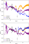 |
Fig. 6 Best fit forward models between 0.3–30 μm, from our retrievals including both HST WFC3 and Spitzer IRAC data, indicating some absorption features which could be identified from transmission spectra of future missions such as JWST or ARIEL. Top: H2O only, AlO only, and H2O + AlO. Bottom: H2O only, H2O + CO2, and H2O + CO2 + AlO. The HST WFC3 and Spitzer IRAC data are included for reference. |
4.5 Comparison to previous work
Our simplest model includes H2O and AlO only and is cloud-free. We can compare the retrieved parameters that are given in Fig. 3 to previous studies of the same transmission spectra. We retrieve a temperature of  K, compared to
  K from Kreidberg et al. (2014). Another study of 30 exoplanets from Tsiaras et al. (2018) yielded 957 ± 343 K for WASP-43b, which used the transmission spectra generated from their own data reduction methods. This same data for WASP-43b was used by Fisher & Heng (2018) in a recent study of 38 exoplanets; they retrieved a temperature of
  K.
K.
Our retrieved molecular abundances (within 1σ ranges) are 2.9 × 10⁻⁷–3.8 × 10⁻³ and 7.6 × 10⁻⁸–4.2 × 10⁻⁴ for H2O and AlO, respectively. The water vapour volume mixing ratio was found to be 3.2 × 10⁻⁵–1.6 × 10⁻³ by Kreidberg et al. (2014), 1.1 × 10⁻⁶–1.7 × 10⁻² by Fisher & Heng (2018), 3.5 × 10⁻⁷–5.5 × 10⁻³ by Tsiaras et al. (2018), 3.6 × 10⁻⁵–3.9 × 10⁻² by Weaver et al. (2020), and 1 × 10⁻⁴–1 × 10⁻³ by Irwin et al. (2020). We can only compare the retrieved H2O abundance to previous studies, as AlO was not included in any previous retrievals.
While all the values are roughly in agreement, within the error bars, there are huge uncertainties on the retrieved parameters. We note that there is degeneracy between the retrieved radius, temperature, and molecular abundances. For example, a lower temperaturecan be compensated by a higher radius and higher abundances without much variation in the final spectra. This is sometimes referred to as the “normalisation degeneracy” (see e.g. Benneke & Seager 2012; Griffith 2014; Heng & Kitzmann 2017; Fisher & Heng 2018). As our retrieval is based on HST WFC3 data alone, we are not able to place any tight constraints on the retrieved parameters. Figure 3 does, however, show that there is a positive correlation between H2O and AlO, which means that the ratio of the two should be better constrained than the absolute abundances of each. We can use some approximations to compare this to solar abundances. Based on the solar elemental abundances given in Asplund et al. (2009), solar log(Al/O) = −2.24. We can compare this to our retrieved value of log(AlO/(AlO+H2O)) =  . This is assuming that most of the oxygen is in H2O, and all the aluminium is contained within AlO. In reality, oxygen would likely also be locked into silicate and other species, although this would not be expected to have a significant effect. If Al were contained within other species, this would be lower than the actual abundance of Al/O, but if oxygen were contained in other species our estimate would be higher than the true value.
5 Summary
In this workwe have performed a re-analysis of the HST WFC3 transmission spectrum of WASP-43b between 1.1–1.7 μm. We have tested the statistical significance of including every molecule for which high-temperature opacity data exists in this wavelength region. We find strong evidence (>5σ) to justify the inclusion of AlO and H2O in our model, but not for any other molecules in this region. We investigate the effects of including Spitzer IRAC data points at 3.6 μm and 4.5 μm, and find the inclusion of these points gives strength to our AlO and H2O detection. The presence of AlO at the temperatures and pressures that these transmission observations are probing is not expected from equilibrium chemistry; its presence is therefore evidence of disequilibrium processes in the atmosphere of WASP-43b. Detecting heavy elements such as Al in a planetary atmosphere also gives some insight into planet formation processes (Johnson & Li 2012; Hasegawa & Hirashita 2014). None of the previous studies analysing the transmission spectra of WASP-43b considered AlO as a potential molecule to include in their retrieval process, and only a small set of the molecules for which there is data available were included. It should be noted that the AlO line list was not available when the atmosphere of WASP-43b was first analysed by Kreidberg et al. (2014). Our approach of considering all molecules for which data currently exists highlights the importance of projects such as ExoMol and HITEMP for expanding our knowledge of high-temperature exoplanet atmospheres, in particular in the era of space missions such as JWST and ARIEL. We note that molecular abundances and other retrieved parameters cannot be accurately constrained by WFC3 data alone, as has previously been pointed out by works such as Heng & Kitzmann (2017), and observations across a wide range of wavelengths are essential for expanding on this and other works on WASP-43b.
Acknowledgements
This project has received funding from the European Union’s Horizon 2020 Research and Innovation Programme, under Grant Agreement 776403, and from the European Research Council (ERC) under the European Union’s Horizon 2020 research and innovation programme under grant agreement No 758892, ExoAI. We thank the referee for their constructive comments on the manuscript.
Appendix A Additional retrieval data
Nested sampling global log-evidence (log(E)) of various retrievals of the HST/WFC3 data, along with the natural log of the Bayes factor, ln(B01), and σ likelihood against: a flat “base” retrieval (i.e. with no molecular features), a retrieval with only H2O included, and a retrieval with only AlO included.
Nested sampling global log-evidence (log(E)) of various retrievals of the HST/WFC3 data, with various combinations of including Rayleigh scattering, collision induced absorption (CIA) of H2-He and H2-H2 (Gordon et al. 2017; Borysow et al. 2001), or clouds.
Appendix B Individual ARCiS forward models
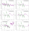 |
Fig. B.1 ARCiS forward models, each including one individual species, plotted alongside the transmission data for WASP-43b from Kreidberg et al. (2014) in order to help assess which molecules to include in subsequent retrievals. |
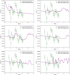 |
Fig. B.1 continued. |
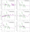 |
Fig. B.1 continued. |
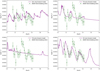 |
Fig. B.1 continued. |
References
- Agúndez, M., Parmentier, V., Venot, O., Hersant, F., & Selsis, F. 2014, A&A, 564, A73 [NASA ADS] [CrossRef] [EDP Sciences] [Google Scholar]
- Al-Refaie, A. F., Yachmenev, A., Tennyson, J., & Yurchenko, S. N. 2015, MNRAS, 448, 1704 [NASA ADS] [CrossRef] [Google Scholar]
- Amaral, P. H. R., Diniz, L. G., Jones, K. A., et al. 2019, ApJ, 878, 95 [CrossRef] [Google Scholar]
- Asplund, M., Grevesse, N., Sauval, A. J., & Scott, P. 2009, ARA&A, 47, 481 [NASA ADS] [CrossRef] [Google Scholar]
- Azzam, A. A. A., Yurchenko, S. N., Tennyson, J., & Naumenko, O. V. 2016, MNRAS, 460, 4063 [NASA ADS] [CrossRef] [Google Scholar]
- Barber, R. J., Strange, J. K., Hill, C., et al. 2014, MNRAS, 437, 1828 [NASA ADS] [CrossRef] [Google Scholar]
- Barton, E. J., Yurchenko, S. N., & Tennyson, J. 2013, MNRAS, 434, 1469 [NASA ADS] [CrossRef] [Google Scholar]
- Bean, J. 2013, Follow The Water: The Ultimate WFC3 Exoplanet Atmosphere Survey, HST Proposal [Google Scholar]
- Benneke, B., & Seager, S. 2012, ApJ, 753, 100 [NASA ADS] [CrossRef] [Google Scholar]
- Bernath, P. F. 2020, J. Quant. Spectr. Rad. Transf., 240, 106687 [CrossRef] [Google Scholar]
- Bittner, D. M., & Bernath, P. F. 2018, ApJS, 235, 8 [NASA ADS] [CrossRef] [Google Scholar]
- Blecic, J., Harrington, J., Madhusudhan, N., et al. 2014, ApJ, 781, 116 [NASA ADS] [CrossRef] [Google Scholar]
- Borysow, A., Jørgensen, U. G., & Fu, Y. 2001, J. Quant. Spectr. Rad. Transf., 68, 235 [NASA ADS] [CrossRef] [Google Scholar]
- Boulangier, J., Gobrecht, D., Decin, L., de Koter, A., & Yates, J. 2019, MNRAS, 489, 4890 [NASA ADS] [CrossRef] [Google Scholar]
- Burrows, A., Dulick, M., C. W. Bauschlicher, J., et al. 2005, ApJ, 624, 988 [NASA ADS] [CrossRef] [Google Scholar]
- Chen, G., van Boekel, R., Wang, H., et al. 2014, A&A, 563, A40 [NASA ADS] [CrossRef] [EDP Sciences] [Google Scholar]
- Chubb, K. L., Rocchetto, M., Yurchenko, S. N., et al. 2020a, A&A, submitted [Google Scholar]
- Chubb, K. L., Tennyson, J., & Yurchenko, S. N. 2020b, MNRAS, 493, 1531 [CrossRef] [Google Scholar]
- Coles, P. A., Yurchenko, S. N., & Tennyson, J. 2019, MNRAS, 490, 4638 [CrossRef] [Google Scholar]
- De Beck, E., Decin, L., Ramstedt, S., et al. 2017, A&A, 598, A53 [NASA ADS] [CrossRef] [EDP Sciences] [Google Scholar]
- Decin, L., Richards, A. M. S., Waters, L. B. F. M., et al. 2017, A&A, 608, A55 [NASA ADS] [CrossRef] [EDP Sciences] [Google Scholar]
- Edwards, B., Rice, M., Zingales, T., et al. 2019, Exp. Astron., 47, 29 [CrossRef] [Google Scholar]
- Feng, Y. K., Line, M. R., Fortney, J. J., et al. 2016, ApJ, 829, 52 [NASA ADS] [CrossRef] [Google Scholar]
- Feroz, F., & Hobson, M. P. 2008, MNRAS, 384, 449 [NASA ADS] [CrossRef] [Google Scholar]
- Feroz, F., Gair, J. R., Hobson, M. P., & Porter, E. K. 2009, Class. Quantum Gravity, 26, 215003 [NASA ADS] [CrossRef] [Google Scholar]
- Feroz, F., Hobson, M. P., Cameron, E., & Pettitt, A. N. 2013, in Importance Nested Sampling and the MultiNest Algorithm [Google Scholar]
- Fisher, C., & Heng, K. 2018, MNRAS, 481, 4698 [Google Scholar]
- Gandhi, S., & Madhusudhan, N. 2017, MNRAS, 474, 271 [NASA ADS] [CrossRef] [Google Scholar]
- Gandhi, S., & Madhusudhan, N. 2019, MNRAS, 485, 5817 [NASA ADS] [CrossRef] [Google Scholar]
- Gardner, J. P., Mather, J. C., Clampin, M., et al. 2006, Space Sci. Rev., 123, 485 [NASA ADS] [CrossRef] [Google Scholar]
- Gillon, M., Triaud, A. H. M. J., Fortney, J. J., et al. 2012, A&A, 542, A4 [NASA ADS] [CrossRef] [EDP Sciences] [Google Scholar]
- Gordon, I. E., Rothmana, L. S., Hill, C., et al. 2017, J. Quant. Spectr. Rad. Transf., 203, 3 [Google Scholar]
- Griffith, C. A. 2014, Phil. Trans. R. Soc. A Math. Phys. Eng. Sci., 372, 20130086 [NASA ADS] [CrossRef] [Google Scholar]
- Hasegawa, Y., & Hirashita, H. 2014, ApJ, 788, 62 [NASA ADS] [CrossRef] [Google Scholar]
- Hellier, C., Anderson, D. R., Collier Cameron, A., et al. 2011, A&A, 535, L7 [NASA ADS] [CrossRef] [EDP Sciences] [Google Scholar]
- Helling, C., Lee, G., Dobbs-Dixon, I., et al. 2016, MNRAS, 460, 855 [NASA ADS] [CrossRef] [Google Scholar]
- Helling, C., Iro, N., Corrales, L., et al. 2019, A&A, 631, A79 [NASA ADS] [CrossRef] [EDP Sciences] [Google Scholar]
- Helling, C., Graham, V., Samra, D., et al. 2020, A&A, submitted [Google Scholar]
- Heng, K., & Kitzmann, D. 2017, MNRAS, 470, 2972 [NASA ADS] [CrossRef] [Google Scholar]
- Hou, S., & Bernath, P. F. 2018, J. Quant. Spectr. Rad. Transf., 210, 44 [CrossRef] [Google Scholar]
- Irwin, P. G. J., Parmentier, V., Taylor, J., et al. 2020, MNRAS, 493, 106 [CrossRef] [Google Scholar]
- Johnson, J. L., & Li, H. 2012, ApJ, 751, 81 [NASA ADS] [CrossRef] [Google Scholar]
- Kataria, T., Showman, A. P., Fortney, J. J., et al. 2015, ApJ, 801, 86 [NASA ADS] [CrossRef] [Google Scholar]
- Keating, D., & Cowan, N. B. 2017, ApJ, 849, L5 [Google Scholar]
- Komacek, T. D., Showman, A. P., & Tan, X. 2017, ApJ, 835, 198 [NASA ADS] [CrossRef] [Google Scholar]
- Kramida, A., Ralchenko, Y., & Reader, J. 2013, NIST Atomic Spectra Database – Version 5 [Google Scholar]
- Kreidberg, L., Bean, J. L., Désert, J.-M., et al. 2014, ApJ, 793, L27 [NASA ADS] [CrossRef] [Google Scholar]
- Langleben, J., Tennyson, J., Yurchenko, S. N., & Bernath, P. 2019, MNRAS, 488, 2332 [CrossRef] [Google Scholar]
- Li, G., Gordon, I. E., Rothman, L. S., et al. 2015, ApJS, 216, 15 [NASA ADS] [CrossRef] [Google Scholar]
- Li, H. Y., Tennyson, J., & Yurchenko, S. N. 2019, MNRAS, 486, 2351 [CrossRef] [Google Scholar]
- Lodi, L., Yurchenko, S. N., & Tennyson, J. 2015, Mol. Phys., 113, 1998 [NASA ADS] [CrossRef] [Google Scholar]
- Louden, T., & Kreidberg, L. 2018, MNRAS, 477, 2613 [NASA ADS] [CrossRef] [Google Scholar]
- Mant, B. P., Yachmenev, A., Tennyson, J., & Yurchenko, S. N. 2018, MNRAS, 478, 3220 [CrossRef] [Google Scholar]
- Masseron, T., Plez, B., Van Eck, S., et al. 2014, A&A, 571, A47 [NASA ADS] [CrossRef] [EDP Sciences] [Google Scholar]
- McKemmish, L. K., Yurchenko, S. N., & Tennyson, J. 2016, MNRAS, 463, 771 [NASA ADS] [CrossRef] [Google Scholar]
- McKemmish, L. K., Masseron, T., Hoeijmakers, J., et al. 2019, MNRAS, 488, 2836 [NASA ADS] [CrossRef] [Google Scholar]
- Mendonça, J. M., min Tsai, S., Malik, M., Grimm, S. L., & Heng, K. 2018a, ApJ, 869, 107 [NASA ADS] [CrossRef] [Google Scholar]
- Mendonça, J. M., Malik, M., Demory, B.-O., & Heng, K. 2018b, AJ, 155, 150 [CrossRef] [Google Scholar]
- Min, M., Hovenier, J. W., & de Koter, A. 2005, A&A, 432, 909 [NASA ADS] [CrossRef] [EDP Sciences] [Google Scholar]
- Min, M., Ormel, C. W., Chubb, K. L., Helling, C., & Kawashima, Y. 2020, A&A, (in revision) [Google Scholar]
- Mollière, P., van Boekel, R., Dullemond, C., Henning, T., & Mordasini, C. 2015, ApJ, 813, 47 [NASA ADS] [CrossRef] [Google Scholar]
- Morello, G., Danielski, C., Dickens, D., Tremblin, P., & Lagage, P.-O. 2019, AJ, 157, 205 [CrossRef] [Google Scholar]
- Murgas, F., Pallé, E., Zapatero Osorio, M. R., et al. 2014, A&A, 563, A41 [NASA ADS] [CrossRef] [EDP Sciences] [Google Scholar]
- Ormel, C. W., & Min, M. 2019, A&A, 622, A121 [NASA ADS] [CrossRef] [EDP Sciences] [Google Scholar]
- Parmentier, V., Fortney, J. J., Showman, A. P., Morley, C., & Marley, M. S. 2016, ApJ, 828, 22 [NASA ADS] [CrossRef] [Google Scholar]
- Pascale, E., Bezawada, N., Barstow, J., et al. 2018, Proc. SPIE 10698, 169 [Google Scholar]
- Patrascu, A. T., Hill, C., Tennyson, J., & Yurchenko, S. N. 2014, J. Chem. Phys., 141, 144312 [CrossRef] [Google Scholar]
- Patrascu, A. T., Yurchenko, S. N., & Tennyson, J. 2015, MNRAS, 449, 3613 [NASA ADS] [CrossRef] [Google Scholar]
- Pavlyuchko, A. I., Yurchenko, S. N., & Tennyson, J. 2015, MNRAS, 452, 1702 [CrossRef] [Google Scholar]
- Polyansky, O. L., Kyuberis, A. A., Zobov, N. F., et al. 2018, MNRAS, 480, 2597 [NASA ADS] [CrossRef] [Google Scholar]
- Prajapat, L., Jagoda, P., Lodi, L., et al. 2017, MNRAS, 472, 3648 [CrossRef] [Google Scholar]
- Rothman, L. S., Gordon, I. E., Barber, R. J., et al. 2010, J. Quant. Spectr. Rad. Transf., 111, 2139 [NASA ADS] [CrossRef] [Google Scholar]
- Stevenson, K. B., Harrington, J., Nymeyer, S., et al. 2010, Nature, 464, 1161 [NASA ADS] [CrossRef] [PubMed] [Google Scholar]
- Stevenson, K. B., Désert, J.-M., Line, M. R., et al. 2014, Science, 346, 838 [NASA ADS] [CrossRef] [Google Scholar]
- Stevenson, K. B., Line, M. R., Bean, J. L., et al. 2017, ApJ, 153, 68 [Google Scholar]
- Takigawa, A., Kamizuka, T., Tachibana, S., & Yamamura, I. 2017, Sci. Adv., 3, 2149 [CrossRef] [Google Scholar]
- Tennyson, J., & Yurchenko, S. N. 2018, Atoms, 6, 26 [NASA ADS] [CrossRef] [Google Scholar]
- Tennyson, J., Yurchenko, S. N., Al-Refaie, A. F., et al. 2016, J. Mol. Spectr., 327, 73 [NASA ADS] [CrossRef] [Google Scholar]
- Trotta, R. 2008, Contemp. Phys., 49, 71 [Google Scholar]
- Tsiaras, A., Waldmann, I. P., Zingales, T., et al. 2018, AJ, 155, 156 [NASA ADS] [CrossRef] [Google Scholar]
- Valyavin, G. G., Gadelshin, D. R., Valeev, A. F., et al. 2018, Astrophys. Bull., 73, 225 [CrossRef] [Google Scholar]
- Venot, O., Parmentier, V., Blecic, J., et al. 2020, ApJ, 890, 176 [CrossRef] [Google Scholar]
- von Essen, C., Mallonn, M., Welbanks, L., et al. 2019, A&A, 622, A71 [NASA ADS] [CrossRef] [EDP Sciences] [Google Scholar]
- Waldmann, I. P., Tinetti, G., Rocchetto, M., et al. 2015, ApJ, 802, 107 [NASA ADS] [CrossRef] [Google Scholar]
- Wang, Y., Tennyson, J., & Yurchenko, S. N. 2020, Atoms, 8, 7 [CrossRef] [Google Scholar]
- Weaver, I. C., López-Morales, M., Espinoza, N., et al. 2020, AJ, 159, 13 [Google Scholar]
- Wende, S., Reiners, A., Seifahrt, A., & Bernath, P. F. 2010, A&A, 523, A58 [NASA ADS] [CrossRef] [EDP Sciences] [Google Scholar]
- Woitke, P., Helling, C., Hunter, G. H., et al. 2018, A&A, 614, A1 [NASA ADS] [CrossRef] [EDP Sciences] [Google Scholar]
- Yousefi, M., & Bernath, P. F. 2018, ApJS, 237, 8 [CrossRef] [Google Scholar]
- Yousefi, M., Bernath, P. F., Hodges, J., & Masseron, T. 2018, J. Quant. Spectr. Rad. Transf., 217, 416 [Google Scholar]
- Yurchenko, S. N., Amundsen, D. S., Tennyson, J., & Waldmann, I. P. 2017, A&A, 605, A95 [NASA ADS] [CrossRef] [EDP Sciences] [Google Scholar]
- Yurchenko, S. N., Al-Refaie, A. F., & Tennyson, J. 2018a, A&A, 614, A131 [NASA ADS] [CrossRef] [EDP Sciences] [Google Scholar]
- Yurchenko, S. N., Bond, W., Gorman, M. N., et al. 2018b, MNRAS, 478, 270 [CrossRef] [Google Scholar]
- Yurchenko, S. N., Williams, H., Leyland, P. C., Lodi, L., & Tennyson, J. 2018c, MNRAS, 479, 1401 [CrossRef] [Google Scholar]
All Tables
Reduced χ2 for different combinations of molecules (in addition to H2O) included in a cloud-free retrieval using ARCiS, and references for the line lists used.
Nested sampling global log-evidence (log(E)) of various retrievals of the HST/WFC3 data, along with the natural log of the Bayes factor, ln(B01), and σ likelihood against: a flat “base” retrieval (i.e. with no molecular features), a retrieval with only H2O included, and a retrieval with only AlO included.
Nested sampling global log-evidence (log(E)) of various retrievals of the HST/WFC3 data, along with the natural log of the Bayes factor, ln(B01), and σ likelihood against: a flat “base” retrieval (i.e. with no molecular features), a retrieval with only H2O included, and a retrieval with only AlO included.
Nested sampling global log-evidence (log(E)) of various retrievals of the HST/WFC3 data, with various combinations of including Rayleigh scattering, collision induced absorption (CIA) of H2-He and H2-H2 (Gordon et al. 2017; Borysow et al. 2001), or clouds.
All Figures
|
Fig. 1 Cloud-free Tau-REx transmission retrieval results with H2O and AlO (top) and with H2O only (bottom). The different shading corresponds to 1σ and 2σ regions. |
| In the text | |
|
Fig. 2 Contributions of molecular features to the cloud-free Tau-REx retrieval results that include AlO and H2O only. |
| In the text | |
|
Fig. 3 TauRex transmission retrieval posteriors for H2O and AlO, with no clouds. |
| In the text | |
|
Fig. 4 Tau-REx transmission retrieval results, including Spitzer points from Blecic et al. (2014), with H2O and AlO (top) and the contributions of each molecule to the retrieval result (bottom). The different shading in the first panel corresponds to 1σ and 2σ regions. |
| In the text | |
|
Fig. 5 Tau-REx transmission retrieval results, including Spitzer points from Blecic et al. (2014), with H2O and CO2 (top) and the contributions of each molecule to the retrieval result (bottom). The different shading in the first panel corresponds to 1σ and 2σ regions. |
| In the text | |
|
Fig. 6 Best fit forward models between 0.3–30 μm, from our retrievals including both HST WFC3 and Spitzer IRAC data, indicating some absorption features which could be identified from transmission spectra of future missions such as JWST or ARIEL. Top: H2O only, AlO only, and H2O + AlO. Bottom: H2O only, H2O + CO2, and H2O + CO2 + AlO. The HST WFC3 and Spitzer IRAC data are included for reference. |
| In the text | |
|
Fig. B.1 ARCiS forward models, each including one individual species, plotted alongside the transmission data for WASP-43b from Kreidberg et al. (2014) in order to help assess which molecules to include in subsequent retrievals. |
| In the text | |
|
Fig. B.1 continued. |
| In the text | |
|
Fig. B.1 continued. |
| In the text | |
|
Fig. B.1 continued. |
| In the text | |
Current usage metrics show cumulative count of Article Views (full-text article views including HTML views, PDF and ePub downloads, according to the available data) and Abstracts Views on Vision4Press platform.
Data correspond to usage on the plateform after 2015. The current usage metrics is available 48-96 hours after online publication and is updated daily on week days.
Initial download of the metrics may take a while.