© ESO 2020

1 Introduction

Astronomical datasets, like most datasets, are contaminated by various sources of noise, such as photon noise, the intrinsic variability of the object of interest, contamination by the Earth’s atmosphere, instrumental noise, etc. While the photon noise is purely white (i.e., uncorrelated), most of the other sources of noise have temporal or spatial correlations. When neglected, these correlations can lead to spurious signal detections.

In the context of exoplanet detection with radial velocity time series, stellar variability could induce signals that mimic planetary signatures (e.g., Queloz et al. 2001). The mitigation of stellar variability has become a major subject in planet search studies and is now routinely achieved by modeling it as correlated Gaussian noise. Adopting such models significantly improves the robustness of planet detection (e.g., Haywood et al. 2014; Rajpaul et al. 2015; Faria et al. 2016). Correlated noise also affects the determination of a planet’s parameters and can induce, in particular, spurious eccentricities when it is not properly accounted for (e.g., Hara et al. 2019).

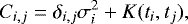
In many cases, the physical processes inducing correlated noise cannot be modeled precisely but qualitative properties, typical timescales, and amplitudes can be estimated. Thus, a common approach is to use simple parametric noise models. For a time series of size n with observations taken at times t_i (i < n), the covariance matrix of the noise is typically modeled as: $$C_{i,j}={\delta }_{i,j}{\sigma }_i^2+K(t_i,t_j),$$(1)

where σ_i are individual errorbars (e.g., photon noise) and K is the kernel of the correlated noise. The noise is often assumed to be stationary, such that K(t_i, t_j) only depends on |t_i − t_j|, $$K(t_i,t_j)=k(|t_i-t_j|).$$(2)

A simple, widespread model assumes the correlation to decrease exponentially with time, with a timescale of τ, $$k(\Delta t)={\sigma }_{\text{corr}.}^2{e}^{-\frac{\Delta t}{\tau }},$$(3)

but it is sometimes chosen to decrease as a squared exponential (Schwarzenberg-Czerny 1991), $$k(\Delta t)={\sigma }_{\text{corr}.}^2{e}^{-\frac{\Delta t^2}{2{\tau }^2}},$$(4)

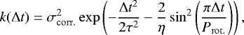
or other similar functions. Slightly more complex models have also been proposed, for instance, quasiperiodic kernels, such as that of Haywood et al. (2014) $$k(\Delta t)={\sigma }_{\text{corr}.}^2\exp \left(-\frac{\Delta t^2}{2{\tau }^2}-\frac{2}{\eta }{\sin }^2\left(\frac{\pi \Delta t}{P_{\text{rot}.}}\right)\right),$$(5)

which allow for a more flexible modeling of the underlying physical processes.

In the case of a poorly understood noise source, the choice of a kernel is somewhat arbitrary but nonetheless, it should be governed by the qualitative properties that the noise is expected to present (typical timescales, periodicities, etc.). For instance, quasiperiodic kernels are well-suited to model the radial velocity signal induced by stellar spots coming in and out of view due to the rotation of the star (see Haywood et al. 2014). Even if the connection to the exact physics of the process is loose, the qualitative properties of quasiperiodic kernels are sufficient to bring a significant improvement in detection reliability.

While correlated noise models improve detection robustness, they might be prohibitive in terms of computational cost and memory footprint. Indeed, for a dataset of size n, the covariance matrix of the noise is of size n × n. In the general case, the memory footprint of storing C is thus $\mathcal{O}\left(n^2\right)$. Then some operations must be performed with this matrix to compute useful quantities (such as the χ² or the likelihood of a model). 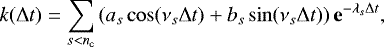The computational cost of these operations (e.g., inversion, dot product, determinant) typically scales as $\mathcal{O}\left(n^2\right)$ to $\mathcal{O}\left(n^3\right)$ in the general case. These scalings make a correct modeling of the noise intractable for large datasets. To address this issue, Ambikasaran (2015) and Foreman-Mackey et al. (2017) proposed a flexible parametric noise model, which allow a linear scaling of the memory footprint and computational cost of the correlated noise. This so-called celerite model is capable of handling a mixture of quasiperiodic covariance kernels of the form: $$k(\Delta t)={\sum }_{s<n_{\text{c}}}\left(a_s\cos ({\nu }_s\Delta t)+b_s\sin ({\nu }_s\Delta t)\right)e^{-{\lambda }_s\Delta t},$$(6)

where n_c is an arbitrarily high number of components in the model. This model has the property to be semiseparable, which allows a scaling of the computational cost as $\mathcal{O}\left(n{n}_{\text{c}}^2\right)$ (Ambikasaran 2015). It is similar to the quasiperiodic kernel of Haywood et al. (2014) which is detailed in Eq. (5). The celerite model is well-suited to represent stellar signals modulated by the rotation period of the star (e.g., Foreman-Mackey et al. 2017). It has been used, in particular, for the analysis of radial velocity and photometric time series.

The star is not the only source of noise in the data. Instruments also introduce a correlated signature. For instance, for precise radial velocity time series (and in other fields), the instrument must be calibrated periodically, typically once per night. Several scientific measurements might use the same calibration and, therefore, share the same calibration noise. The covariance matrix of the calibration noise is then block-diagonal with the blocks corresponding to each calibration (each night). This calibration noise is not stationary and, thus, it is not well represented by the celerite model (see Eq. (6)). More generally, when considering various sources of noise together, the complete covariance matrix might present quasiperiodic components and sparse (block diagonal, banded, etc.) components. While efficient dedicated algorithms exist for both quasiperiodic (semiseparable) and sparse covariance matrices, they cannot be applied in a straightforward way for a mixture of both.

In this article, we extend the method described by Foreman-Mackey et al. (2017) to correlated noise with a semiseparable component plus a sparse component. We introduce the notion of LEAF matrices, a general class of sparse, “close to diagonal” symmetric matrices encompassing banded, block-diagonal, staircase matrices, etc. Our complete model, which we call the S + LEAF model, is the sum of a semiseparable component and a LEAF component.

In Sect. 2, we present the S + LEAF correlated noise model and dedicated algorithms. In Sect. 3, we illustrate our methods using the HARPS radial velocities of HD 136352. We discuss our results in Sect. 4. We provide an open-source reference implementation of S + LEAF matrices and related algorithms as a C library with python wrappers¹.

2 The S + LEAF noise model

The likelihood (i.e., the probability of the data assuming a given model is correct) is a common tool for assessing the agreement of a given model to a dataset. In a Bayesian approach, the quantity of interest is the posterior probability (probability of a model given the data), but the computation of the likelihood is still required as an intermediate step. In this section, we describe the S + LEAF noise model and dedicated algorithms which allow, in particular, for the efficient computation of the likelihood and its derivatives.

In Sect. 2.1, we introduce notations and describe the computation of the likelihood in the general case. We define S + LEAF matrices in Sect. 2.2, and we present dedicated algorithms for S + LEAF matrices in Sect. 2.3.

2.1 Likelihood computation, general case

Let us assume that a given dataset y_i (0 ≤ i < n) can be modeled with a deterministic component (the model) m with parameters θ, and a correlated Gaussian noise component ɛ with parameters α: $$\begin{array}{l}{y}_i=m_i(\theta )+{\varepsilon }_i,\\ \varepsilon ~\mathcal{G}(0,C(\alpha )).\end{array}$$(7)

The log-likelihood of a given set of parameters (θ, α) is read as: $$\begin{array}{ll}\ln \mathcal{L}(\theta ,\alpha )\hfill & =\ln p(y|\theta ,\alpha )\hfill \\ \hfill & =-\frac{1}{2}{(y-m(\theta ))}^{\text{T}}{C}^{-1}(\alpha )(y-m(\theta ))\hfill \\ \hfill & -\frac{1}{2}\ln \det (2\pi C(\alpha )),\hfill \end{array}$$(8)

where C(α) is the n × n covariance matrix of the correlated noise ɛ.

The computational cost of evaluating the log-likelihood obviously depends on the cost of evaluating the model m(θ). However, once the model is obtained, we still have to compute the χ² = r^TC⁻¹r (where r represents the residuals, r = y − m) and the determinant of C.

An efficient and robust way to compute the log-likelihood in the general case is to compute the Cholesky decomposition of C as an intermediate step. By definition, the covariance matrix C is symmetric, positive, and definite. It could, in principle, be singular (only semi-definite) but this would mean that some almost-certain affine relation exists in the noise component. This almost-certain relation could thus be included in the deterministic part of the model. Assuming C to be invertible (non-singular), its Cholesky decomposition can be read as: $$C=LD{L}^{\text{T}},$$(9)

where D is diagonal and L is lower triangular with ones on the diagonal. The classical Cholesky decomposition is actually C = ΛΛ^T, where $\Lambda =L\sqrt{D}$ is also lower triangular. However, we use the alternative form of Eq. (9) throughout the article since this notation is more convenient in our case. The computational cost of the Cholesky decomposition is $\mathcal{O}\left(n^3\right)$ in the general case. Once the Cholesky decomposition is obtained, the determinant of C is easily computed (in $\mathcal{O}\left(n\right)$) since ln detC = lndetD = ∑_i lnD_i. The computation of the χ² is performed in $\mathcal{O}\left(n^2\right)$ in the general case by first solving u = L⁻¹r and then computing u^TDu.

2.2 Symmetric S + LEAF covariance matrix

A common method for improving the computational cost and memory footprint of correlated noise models is to obtain a sparse representation of the covariance matrix and to then use dedicated algorithms for solving, computing the determinant, and other functions that make use of this sparsity. For instance, dedicated representations and algorithms for banded matrices, block-diagonal matrices, etc., exist, allowing for the linear scaling in n of the computational cost and footprint of the model ($\mathcal{O}\left(\alpha n\right)$, where α depends on the bandwidth, block size, etc.). In Delisle et al. (2018), the covariance matrix was truncated and approximated by a banded matrix. This representation improved the computational speed of the Markov chain Monte Carlo (MCMC) algorithm used to compute the posterior densities of the orbital elements and noise parameters.

2.2.1 LEAF matrix

Here we introduce a general class of sparse, “close to diagonal” matrices, called LEAF matrices, that encompasses banded, block-diagonal, staircase matrices, etc. A symmetric LEAF matrix F must verify: $$F_{i,j}=F_{j,i}=0\text{for}j<i-b_i,$$(10)

where b_i is the number of non-zero entries left to the diagonal at line i. A sketch of a symmetric LEAF matrix is shown in Fig. 1.

2.2.2 Semiseparable matrix

For efficient computations (typically linear in n), the covariance matrix does not need to be sparse itself, but it should be expressed as a function of sparse matrices (sum, product, inverse, etc.). For instance, Rybicki & Press (1995) showed that exponential matrices, defined as: $$C_{i,j}=e^{-\lambda \Delta t_{i,j}},$$(11)

with Δt_i,j = |t_i − t_j|, possess a tridiagonal inverse T which can be computed directly, without requiring to compute C first (see Rybicki & Press 1995). While the covariance matrix C is not sparse, using the property C = T⁻¹ allows for a very efficient (i.e., in $\mathcal{O}\left(n\right)$) representation and computation. These exponential matrices (as defined in Eq. (11)) are also a particular example of semiseparable matrices which makes it possible to obtain another sparse representation. Indeed, assuming t to be ordered increasingly, and defining u = e^−λt and v = e^λt (vectors of size n), C can be decomposed as: $$C=1+\left(u{v}^{\text{T}}\right)+\text{triu}\left(v{u}^{\text{T}}\right),$$(12)

where tril (respectively triu) stands for the strictly lower (respectively upper) triangular part. The two sparse representations of the exponential matrix of Eq. (11) (i.e., tridiagonal inverse and semiseparable form) are actually linked one to the other, since the inverse of invertible tridiagonal matrices are rank one semiseparable matrices and vice versa (e.g., Vandebril et al. 2005, and references therein).

More generally, a symmetric semiseparable matrix is defined as: $$C=\text{diag}(A)+\text{tril}\left(U{V}^{\text{T}}\right)+\text{triu}\left(V{U}^{\text{T}}\right),$$(13)

where diag(A) is the diagonal matrix built from the vector A (size n), U, and V are (n × r) matrices, and r is the rank of the semiseparable matrix C. Semiseparable matrices can represent a large class of correlated noise models. For instance, the celerite model (see Eq. (6)) proposed by Foreman-Mackey et al. (2017) can be represented as a semiseparable matrix of rank r = 2n_c, with: 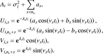$$\begin{array}{l}{A}_i={\sigma }_i^2+{\sum }_{s<n_{\text{c}}}{a}_s,\\ U_{i,s}=e^{-{\lambda }_s{t}_i}\left(a_s\cos ({\nu }_s{t}_i)+b_s\sin ({\nu }_s{t}_i)\right),\\ U_{i,n_{\text{c}}+s}=e^{-{\lambda }_s{t}_i}\left(a_s\sin ({\nu }_s{t}_i)-b_s\cos ({\nu }_s{t}_i)\right),\\ V_{i,s}=e^{{\lambda }_s{t}_i}\cos ({\nu }_s{t}_i),\\ V_{i,n_{\text{c}}+s}=e^{{\lambda }_s{t}_i}\sin ({\nu }_s{t}_i).\end{array}$$(14)

The computational cost and memory footprint of a semiseparable noise model are linear in n (footprint in $\mathcal{O}\left(rn\right)$ and cost in $\mathcal{O}\left(r^{2}n\right)$, see Ambikasaran 2015; Foreman-Mackey et al. 2017).

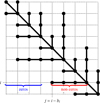Fig. 1 Sketch of a symmetric LEAF matrix.

2.2.3 S + LEAF matrix

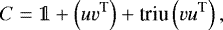
We define a S + LEAF matrix simply as the sum of a semiseparable and a LEAF matrix. A symmetric S + LEAF matrix takes, thus, the form of: $$C=\text{diag}(A)+\text{tril}\left(U{V}^{\text{T}}\right)+\text{triu}\left(V{U}^{\text{T}}\right)+F,$$(15)

where A is a vector of size n representing the diagonalpart of C; U and V are n × r matrices representing the symmetric semiseparable part of C; and F is the symmetric LEAF part of C, as defined in Eq. (10). Since the diagonal part of C is represented by the vector A, we assume the diagonal of F to be filled with zeros. As in Eq. (10), we denote by b_i the number of non-zero entries left to the diagonal, at line i of F (see also Fig. 1). The sparse matrix F can thus be stored in a compact way (i.e., storing only non-zero entries, and using its symmetry) with $\overline{b}n$ values. The memory footprint of the S + LEAF model scales as $\mathcal{O}\left(\left(r+\overline{b}\right)n\right)$ and the computational cost as 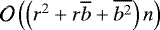$\mathcal{O}\left(\left(r^2+r\overline{b}+\overline{b^2}\right)n\right)$, where r is the number of components in the semiseparable part and for any vector x, $\overline{x}$ stands for the mean of x.

2.3 Likelihood computation with S + LEAF matrices

2.3.1 Cholesky decomposition

We then look for a sparse representation and an efficient computation of the matrices D and L involved in the Cholesky decomposition (see Eq. (9)) of C as defined by Eq. (15). In the case F = 0, Foreman-Mackey et al. (2017) showed that L can be written as: $$L=1+\text{tril}\left(U{W}^{\text{T}}\right),$$(16)

where W is a new n × r matrix which need to be determined. In the case F≠0, this decomposition does not hold but we can prove that there exist a n × r matrix W and a strictly lower triangular LEAF matrix G with the same shape as F (i.e., same values of b_i), such that: 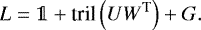$$L=1+\text{tril}\left(U{W}^{\text{T}}\right)+G.$$(17)

Let us first simply assume that G is strictly lower triangular (not necessarily LEAF). In this case, the decomposition is degenerated but always exists. Replacing L by the expression of Eq. (17) in the Cholesky decomposition of C (Eq. (9)) and equating it to Eq. (15), we obtain (for j < i): $$\begin{array}{ll}{C}_{i,i}\hfill & =A_i=D_i+{\sum }_{k<i}{\left({\sum }_s{U}_{i,s}{W}_{k,s}+G_{i,k}\right)}^2{D}_k\hfill \\ \hfill & =D_i+{\sum }_s{U}_{i,s}\left({\sum }_t{S}_{i,s,t}{U}_{i,t}+2Z_{i,i,s}\right)+{\sum }_{k<i}{G}_{i,k}^2{D}_k,\hfill \\ C_{i,j}\hfill & ={\sum }_s{U}_{i,s}{V}_{j,s}+F_{i,j}\hfill \\ \hfill & =\left({\sum }_s{U}_{i,s}{W}_{j,s}+G_{i,j}\right)D_j\hfill \\ \hfill & +{\sum }_{k<j}\left({\sum }_s{U}_{i,s}{W}_{k,s}+G_{i,k}\right)\left({\sum }_t{U}_{j,t}{W}_{k,t}+G_{j,k}\right)D_k\hfill \\ \hfill & ={\sum }_s{U}_{i,s}\left(W_{j,s}{D}_j+{\sum }_t{U}_{j,t}{S}_{j,s,t}+Z_{j,j,s}\right)\hfill \\ \hfill & +G_{i,j}{D}_j+{\sum }_{k<j}{G}_{i,k}{G}_{j,k}{D}_k+{\sum }_s{U}_{j,s}{Z}_{i,j,s},\hfill \end{array}$$

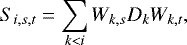
where S is defined following Foreman-Mackey et al. (2017), $$S_{i,s,t}={\sum }_{k<i}{W}_{k,s}{D}_k{W}_{k,t},$$(20)

and Z is defined as: $$Z_{i,j,s}={\sum }_{k<j}{G}_{i,k}{D}_k{W}_{k,s}.$$(21)

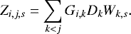
We then break the degeneracy in the expression of L by identifying the terms in front of U_i,s in Eq. (19). Thus we obtain: $$\begin{array}{ll}{V}_{j,s}\hfill & =W_{j,s}{D}_j+{\sum }_t{U}_{j,t}{S}_{j,s,t}+Z_{j,j,s},\hfill \\ F_{i,j}\hfill & =G_{i,j}{D}_j+{\sum }_{k<j}{G}_{i,k}{G}_{j,k}{D}_k+{\sum }_s{U}_{j,s}{Z}_{i,j,s}.\hfill \end{array}$$(22)

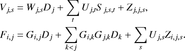
We deduce the following expressions for D, W, and G (for j < i): $$\begin{array}{l}{D}_i=A_i-{\sum }_s{U}_{i,s}\left({\sum }_t{S}_{i,s,t}{U}_{i,t}+2Z_{i,i,s}\right)-{\sum }_{k<i}{G}_{i,k}^2{D}_k,\\ W_{i,s}=\frac{1}{D_i}\left(V_{i,s}-{\sum }_t{S}_{i,s,t}{U}_{i,t}-Z_{i,i,s}\right),\\ G_{i,j}=\frac{1}{D_j}\left(F_{i,j}-{\sum }_{k<j}{G}_{i,k}{G}_{j,k}{D}_k-{\sum }_s{U}_{j,s}{Z}_{i,j,s}\right).\end{array}$$

From Eqs. (21) and (25), we can check by induction that G_i,j = Z_i,j,s = 0 for j < i − b_i. Therefore, G and Z have the same LEAF shape as F, which proves that the decomposition of Eq. (17) always exists.

Using this property, we are able to compute compact recursion formulas for the expression of S, Z, G, D, and W. We find that for increasing values of i and increasing values of j at i fixed (with i − b_i ≤ j < i): $$\begin{array}{l}{S}_{0,s,t}=0,\\ S_{i,s,t}=S_{i-1,s,t}+W_{i-1,s}{D}_{i-1}{W}_{i-1,t}(i>0),\\ Z_{i,i-b_i,s}=0,\\ Z_{i,j,s}=Z_{i,j-1,s}+G_{i,j-1}{D}_{j-1}{W}_{j-1,s}(j>i-b_i),\\ G_{i,j}=\frac{1}{D_j}\left(F_{i,j}-{\sum }_{k=\max (i-b_i,j-b_j)}^{j-1}{G}_{i,k}{G}_{j,k}{D}_k-{\sum }_s{U}_{j,s}{Z}_{i,j,s}\right),\\ D_i=A_i-{\sum }_s{U}_{i,s}\left({\sum }_t{S}_{i,s,t}{U}_{i,t}+2Z_{i,i,s}\right)-{\sum }_{k=i-b_i}^{i-1}{G}_{i,k}^2{D}_k,\\ W_{i,s}=\frac{1}{D_i}\left(V_{i,s}-{\sum }_t{S}_{i,s,t}{U}_{i,t}-Z_{i,i,s}\right).\end{array}$$

While S is a n × r× r tensor, it is not necessary to keep all its values in memory, and S can be stored as a r × r matrix which is updated in place for increasing values of i. The same reasoning holds for Z, which can be stored as a vector of size r, and updated for increasing values of i and j. However, if the backpropagation of the gradient is required, all the values of S and Z should be stored for reasons of stability and performance (see Sect. 2.3.4). In this case, the memory footprint of the S + LEAF model increases but remains linear in n (i.e., $\mathcal{O}\left(\left(r+\overline{b}\right)rn\right)$ instead of $\mathcal{O}\left(\left(r+\overline{b}\right)n\right)$).

2.3.2 Computing the determinant and solving

As explained in Sect. 2.1, once the Cholesky decomposition of the covariance matrix C is known, we need to compute its determinant and solve for x = L⁻¹y to compute the likelihood of a set of parameters. The determinant is trivially obtained in $\mathcal{O}(n)$ operations, $$\ln \det (C)=\ln \det (D)={\sum }_i\ln D_i.$$(31)

We can then describe how to solve for x = L⁻¹y (with L defined as in Eq. (17)). Since y = Lx, we have: $$\begin{array}{ll}{y}_i\hfill & =x_i+{\sum }_{j<i}\left({\sum }_s{U}_{i,s}{W}_{j,s}+G_{i,j}\right)x_j\hfill \\ \hfill & =x_i+{\sum }_s{U}_{i,s}{f}_{i,s}+{\sum }_{j=i-b_i}^{i-1}{G}_{i,j}{x}_j,\hfill \end{array}$$(32)

with f defined as in Foreman-Mackey et al. (2017), $$f_{i,s}={\sum }_{j<i}{W}_{j,s}{x}_j.$$(33)

We thus obtain the following recursion formulas for increasing values of i: $$\begin{array}{l}{f}_{0,s}=0,\\ f_{i,s}=f_{i-1,s}+W_{i-1,s}{x}_{i-1}(i>0),\\ x_i=y_i-{\sum }_s{U}_{i,s}{f}_{i,s}-{\sum }_{j=i-b_i}^{i-1}{G}_{i,j}{x}_j.\end{array}$$

As for the Cholesky factorization, the values of f can be stored in a vector of size r and updated in place for increasing values of i, except in the case where the backpropagation of the gradient is required (see Sect. 2.3.4). The computational cost of this solving is in $\mathcal{O}\left(\left(r+\overline{b}\right)n\right)$.

While it is not needed in the calculation of the likelihood, the computation of the dot product y = Lx is very similar to the solving problem (x = L⁻¹y). For increasing values of i, we compute: $$\begin{array}{l}{f}_{0,s}=0,\\ f_{i,s}=f_{i-1,s}+W_{i-1,s}{x}_{i-1}(i>0),\\ y_i=x_i+{\sum }_s{U}_{i,s}{f}_{i,s}+{\sum }_{j=i-b_i}^{i-1}{G}_{i,j}{x}_j.\end{array}$$

Similar recursion formulas for the dot product y = L^Tx and the solving of x = L^-Ty are easily obtained.

2.3.3 Overflows and preconditioning

As noted byAmbikasaran (2015); Foreman-Mackey et al. (2017), a naive computer implementation of exponential semiseparable matrices can lead to numerical underflows and overflows. Indeed, the separation of the exponential e^{−λ_s|t_i−t_j|} in U_i,s= e^−λ_st_i and V_j,s= e^λ_st_j exhibits very interesting theoretical properties (semiseparable matrix) but in practical applications, λ_s t_i and λ_s t_j can reach values that are much larger than λ_s|t_i − t_j|, which causes underflows for U and overflows for V.

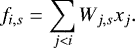
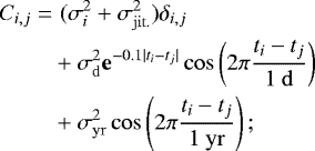
To circumvent this numerical issue, we follow Foreman-Mackey et al. (2017) and introduce the (n − 1) × r preconditioning matrix ϕ, and the preconditioned matrices Ũ and Ṽ, such that $$U_{i,s}{V}_{j,s}={\tilde{U}}_{i,s}{\tilde{V}}_{j,s}{\displaystyle \prod _{k=j}^{i-1}{\varphi }_{k,s}}.$$(38)

For instance, in the case of the celerite model – Eqs. (6) and (14) – Foreman-Mackey et al. (2017) proposed the following preconditioning: $$\begin{array}{l}{\tilde{U}}_{i,s}=a_s\cos ({\nu }_s{t}_i)+b_s\sin ({\nu }_s{t}_i),\\ {\tilde{U}}_{i,n_{\text{c}}+s}=a_s\sin ({\nu }_s{t}_i)-b_s\cos ({\nu }_s{t}_i),\\ {\tilde{V}}_{i,s}=\cos ({\nu }_s{t}_i),\\ {\tilde{V}}_{i,n_{\text{c}}+s}=\sin ({\nu }_s{t}_i),\\ {\varphi }_{i,s}={\varphi }_{i,n_{\text{c}}+s}=e^{-{\lambda }_s(t_{i+1}-t_i)},\end{array}$$(39)

which avoids the computation of exponentials with large exponents. All the algorithms presented above (Cholesky decomposition, dot product and solving) can be adapted to take into account this preconditioning. We refer the reader to Appendix A for more details.

2.3.4 Efficient computation of the likelihood derivatives

Once the model is chosen, we typically need to determine a point estimate or the posterior distribution of the parameters. In order to use efficient optimization or exploration algorithms, it might be useful to compute the gradient of the log-likelihood (Eq. (8)) with respect to the model parameters (θ) and the noise parameters (α). Foreman-Mackey (2018) provided gradient backpropagation algorithms for the Cholesky decomposition, dot product, and solving problem in the case of semiseparable matrices (F = 0 in our notations). These algorithms allow to very efficiently compute (in $\mathcal{O}\left(r^{2}n\right)$, see Foreman-Mackey 2018) the gradient of the log-likelihood using analytical formulas. The generalization of this method to S + LEAF matrices is straightforward and we provide more details in Appendix B.

3 Application to the analysis of radial velocities

In this section, we illustrate the use of the S + LEAF noise model by reanalyzing the HARPS radial velocity time series of HD 136352 (see Udry et al. 2019). The star HD 136352 is a quiet G4V star known to host three super-Earth planets, at periods of 11.5824 d, 27.5821 d, and 107.6 d, and with minimum masses of 4.8, 10.8, and 8.6 M_⊕ respectively (see Udry et al. 2019). These results were obtained by binning the data and only searching for planets with periods above 1 d. This is a common practice that allows to damp many instrumental and stellar short-term variations (Dumusque et al. 2011). However, it does not allow us to characterize these short-term variations and to fully correct for them. Moreover, binning the data could significantly damp the amplitude of short period planets. Here we reanalyze the raw radial velocities and do not restrict our study to periods above 1 d.

The radial velocities of HD 136352 taken with HARPS consist of 648 points, taken over almost 11 yr (2004–2015), and spread over 238 distinct nights. The number of points per night varies between one and ten, with an average of 2.7 points per night.

We describe the different noise models we use for our study in Sect. 3.1 and present our reanalysis of the HD 136352 system in Sect. 3.2.

3.1 Noise models

To illustratethe role of each component in our S + LEAF noise model, we analyze the data using five different noise models:

• 1.

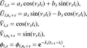
  diag.: a diagonal matrix, with the observational errorbars σ_i plus a jitter term (σ_jit.) added inquadrature (same value for all data points) $$C_{i,j}=({\sigma }_i^2+{\sigma }_{\text{jit}.}^2){\delta }_{i,j};$$(40)

• 2.

  bin.: same as diag. but using nightly binned radial velocity data;

• 3.

  celerite: same as diag. plus quasiperiodic terms at 1 d and 1 yr, $$\begin{array}{ll}{C}_{i,j}=\hfill & ({\sigma }_i^2+{\sigma }_{\text{jit}.}^2){\delta }_{i,j}\hfill \\ \hfill & +{\sigma }_{\text{d}}^2{e}^{-0.1|t_i-t_j|}\cos \left(2\pi \frac{t_i-t_j}{1 \text{d}}\right)\hfill \\ \hfill & +{\sigma }_{\text{yr}}^2\cos \left(2\pi \frac{t_i-t_j}{1 \text{yr}}\right);\hfill \end{array}$$(41)

• 4.

  LEAF: same as diag. but the estimated calibration error ${\sigma }_{b_i}$ (which is part of the observational error σ_i) is shared by night blocks (identified by b_i), and an additional calibration error term (σ_cal.) is added in quadrature to these blocks (same value for all blocks), 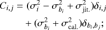$$\begin{array}{ll}{C}_{i,j}=\hfill & ({\sigma }_i^2-{\sigma }_{b_i}^2+{\sigma }_{\text{jit}.}^2){\delta }_{i,j}\hfill \\ \hfill & +({\sigma }_{b_i}^2+{\sigma }_{\text{cal}.}^2){\delta }_{b_i,b_j};\hfill \end{array}$$(42)

• 5.

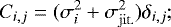
  S + LEAF: same as LEAF plus the two quasiperiodic terms at 1 d and 1 yr as in the celerite model, 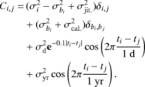$$\begin{array}{ll}{C}_{i,j}=\hfill & ({\sigma }_i^2-{\sigma }_{b_i}^2+{\sigma }_{\text{jit}.}^2){\delta }_{i,j}\hfill \\ \hfill & +({\sigma }_{b_i}^2+{\sigma }_{\text{cal}.}^2){\delta }_{b_i,b_j}\hfill \\ \hfill & +{\sigma }_{\text{d}}^2{e}^{-0.1|t_i-t_j|}\cos \left(2\pi \frac{t_i-t_j}{1 \text{d}}\right)\hfill \\ \hfill & +{\sigma }_{\text{yr}}^2\cos \left(2\pi \frac{t_i-t_j}{1 \text{yr}}\right).\hfill \end{array}$$(43)

The quasiperiodic terms of the celerite and S + LEAF models are modeled according to Eq. (6) and could represent instrumental systematics (CCD stitching, wavelength solution instabilities, incorrect BERV correction, incorrect airmass corrections, etc.; see Dumusque et al. 2015). The HARPS radial velocities of HD 136352 are already corrected from the CCD stitching issue using the method of Dumusque et al. (2015), but remaining systematics could still be present. The amplitudes of the cosines (a_s in Eq. (6)) are noted σ_d and σ_yr. For the sake of simplicity, we fix the amplitudes of the sines to zero (b_s = 0), such that the correlation is always maximum for Δt = 0 (see Eq. (6)). The exponential decay timescale is fixed to 10 d for the daily term (λ_d = 1∕10) and is infinite for the yearly term (λ_yr = 0).

The noise parameters that remain to be determined are, thus, $\alpha =({\sigma }_{\text{jit}.}^2,{\sigma }_{\text{cal}.}^2,{\sigma }_{\text{d}}^2,{\sigma }_{\text{yr}}^2)$, or a subset of it depending on the chosen noise model. The components of the covariance matrices corresponding to each of these four parameters are illustrated in Fig. 2. For these illustrations, the matrices are expanded as full n × n matrices, but we use their sparse representation (as described in Sect. 2) in the following computations.

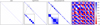Fig. 2 Shapes of the four components of the noise models used for the analysis of the HD 136352 system (Sect. 3).

3.2 Reanalysis of the HD 136352 system

We analyze the HARPS radial velocity time series of HD 136352 using each of the five noise models of Sect. 3.1. The deterministic part of the model is read as: 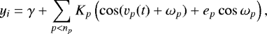$$y_i=\gamma +{\sum }_{p<n_p}{K}_p\left(\cos (v_p(t)+{\omega }_p)+e_p\cos {\omega }_p\right),$$(44)

where γ is the velocity offset, n_p is the number of planets, and, for each planet p, K_p is its semi-amplitude, v_p its true anomaly, e_p its eccentricity, and ω_p its argument of periastron. We start our study by considering a model without any planet and add them gradually, one after the other, by computing a periodogram of the residuals. At each step of this process, we adjust all the free parameters (deterministic and noise parameters). The deterministic parameters (vector θ) are the offset γ and the orbital parmeters P, K, M₀ (mean anomaly at a reference epoch), e, and ω for each planet included in the model. The noise parameters α are a subset of 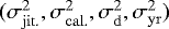$({\sigma }_{\text{jit}.}^2,{\sigma }_{\text{cal}.}^2,{\sigma }_{\text{d}}^2,{\sigma }_{\text{yr}}^2)$ depending on the chosen noise model. We use the L-BFGS-B algorithm (Byrd et al. 1995) to maximize the likelihood (Eq. (8)) and we make use of the backpropagation algorithms described in Sect. 2.3.4 (see also Appendix B) to compute the derivatives of the log-likelihood with respect to the free parameters. We also use classical analytical expressions for the derivatives of the Keplerian model (Eq. (44)) with respect to the orbital parameters of the planets. Then we compute a periodogram of the residuals of this maximum likelihood solution. The offset γ is readjusted for each frequency explored in the periodogram, but the previous planets and noise parameters are fixed (at the values obtained with the last fit).

We compute the periodograms and associated false alarm probability (FAP) using the analytical method of Delisle et al. (2020), based on the previous work by Baluev (2008). For a frequency ν, we define the normalized power as: 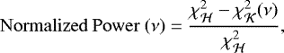$$\text{Normalized}\text{Power}(\nu )=\frac{{\chi }_{\mathcal{H}}^2-{\chi }_{\mathcal{K}}^2(\nu )}{{\chi }_{\mathcal{H}}^2},$$(45)

which corresponds to the definition of the Generalized Lomb-Scargle periodogram (GLS, see Ferraz-Mello 1981; Zechmeister & Kürster 2009), and to $(2/n_{\mathcal{H}})z_1(\nu )$ in the notations of Baluev (2008) and Delisle et al. (2020). In this definition, $\mathcal{H}$ stands for the base model (only the offset γ is adjusted) and $\mathcal{K}$ stands for the model with frequency ν (γ plus the amplitudes of the sine and cosine at frequency ν are adjusted). The χ² of a model m(θ) is defined as: 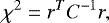$${\chi }^2=r^T{C}^{-1}r,$$(46)

where r is the vector of the model residuals (r = y − m(θ)).

The resulting periodograms are shown in Fig. 3. For the sake of readability, we do not show the first two periodograms since the first two planets (at 11.5824 d and 27.5821 d) are unambiguously detected (highest peaks and FAP < 10⁻¹⁰) independently of the noise model. We additionally provide in Table 1 the values of the noise parameters used to compute each of the periodograms of Fig. 3.

We observe in Fig. 3 (left column) that the last planet (HD 136352 d) is well revovered (highest peak and low FAP) by all models except the celerite model. With the celerite model, the peak corresponding to the planet is not the highest peak and the FAP is high (0.4). We see in Table 1, that the amplitude of the daily quasiperiodic term of the celerite model is adjusted to a high value (3.23 m² s⁻²). On the contrary, for the S + LEAF model, the amplitude of the noise is shared between the daily quasiperiodic term (1.69 m² s⁻²) and the calibration noise (0.56 m² s⁻²). It thus seems that the daily quasiperiodic term of the celerite model is overestimated due to the presence of the unmodeled calibration noise. This shows that the way the calibration noise is accounted for in the S + LEAF model is well suited and does correspond to the behavior of the HARPS instrument.

The periodograms of the residuals of HD 136352 after subtracting all known planets (Fig. 3, right) do not show any significant peak for the celerite (FAP = 0.168) and S + LEAF (FAP = 0.213) models. On the contrary, the diag., bin., and LEAF models show significant peaks (with a low FAP) around 0.5 sd and 1 sd, as well as around 1 yr (see Fig. 3, right). These signals could be of planetary origin but are more probably due to instrumental systematics (CCD stitching, wavelength solution instabilities, incorrect BERV correction, incorrect airmass corrections, etc.; see Dumusque et al. 2015). They could also originate from a combination of stellar correlated noise and aliasing. These potential systematics are taken into account in the celerite and S + LEAF models withthe daily and yearly quasiperiodic terms. While the amplitude of the daily quasiperiodic term is adjusted to significant values in the celerite and S + LEAF models, the amplitude of the yearly quasiperiodic term is completely negligible in both cases (see Table 1). We performed a similar analysis on the HARPS radial velocities of HD 136352 without the stitching correction and obtained higher values for the yearly term (${\sigma }_{\text{yr}}^2\approx 0.25{\text{m}}^2{\text{s}}^{-2}$). This highlights the improvements in the radial velocities obtained with this correction. In the S + LEAF model, the final levels (after substracting all known planets) of the daily quasiperiodic term and the calibration term are of the same order of magnitude (respectively, 0.7 and 0.78 m² s⁻², see Table 1). This provides a good illustration of the importance of taking into account both components in the noise model.

The modeling of the systematics using daily and yearly quasiperiodic terms is a rough approximation, and a further investigation is necessary to confirm that these signals are instrumental systematics, to better characterize the systematics for several systems, to understand the mechanisms that might introduce them, and to correct for them, ideally directly in the HARPS data reduction software (DRS). However, this is beyond the scope of this study, and we simply highlight the ability of the S + LEAF model to roughly account for these systematics.

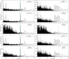Fig. 3 Periodograms of the radial velocity residuals of HD 136352 after subtracting the two first planets (at 11.5824 d and 27.5821 d, left), and after subtracting the three known planets (11.5824 d, 27.5821 d, and 107.6 d right), for the fivenoise models defined in Sect. 3.1. The noise parameters are set to the values provided in Table 1. The vertical blue line highlights the period of the third planet (107.6 d), and the dashed blue lines highlight its aliases at 1 yr. The dotted vertical red lines highlight 0.5 sd, 1 sd, and 1 yr. For the sake of readability, we do not show here the two first periodograms (raw time series and after subtracting the first planet), since the two first planets (11.5824 d and 27.5821 d) are unambiguously detected (highest peaks and FAP < 10−10) independently of the noise model. Assuming that the 107.6 d signal is due to a planet while the signals at 0.5 sd, 1 sd, and around 1 yr are due to correlated noise, we expect the correct noise model to show a low FAP in the left column and a high FAP in the right column.

4 Conclusion

In this article, we present the S + LEAF correlated noise model. While in the general case, accounting for correlated noise in a dataset of size n has a cost of $\mathcal{O}\left(n^3\right)$ and a footprint of $\mathcal{O}\left(n^2\right)$, the S + LEAF noise model scales linearly (i.e., in $\mathcal{O}\left(n\right)$). This linear scaling is made possible by the sparse properties of the S + LEAF covariance matrices (see Sect. 2). The S + LEAF model incorporates a mixture of quasiperiodic components (see Eq. (6)) as the celerite model (Foreman-Mackey et al. 2017) but it additionally takes into account a LEAF component. We call LEAF matrix a general class of “close to diagonal” matrices which encompasses banded, block-diagonal, and staircase matrices (see Eq. (10) and Fig. 1). For instance, the LEAF component of our model is well suited to account for calibration noise in radial velocity time series.

We illustrate the use of the S + LEAF model in the context of radial velocity time series but the model is more general and could be adapted to other fields. We reanalyze the HARPS radial velocity time series of HD 136352 using different noise models (see Sect. 3.2) and observe that the periodograms and FAP levels strongly depend on the chosen noise model. We find that neglecting the short term correlated noise (short period quasiperiodic noise or calibration noise) can lead to spurious detections of signals (underestimation of the FAP), or to a poor detection power (over estimation of the FAP). We thus show that the calibration noise, which can be included in the S + LEAF model, has a substantial effect on detections.

Acknowledgements

We thank the anonymous referee for their useful comments. We thank X. Dumusque and C. Lovis for fruitful discussions, and V. Bourrier for finding the name LEAF while advocating against the use of S + LEAF. We acknowledge financial support from the Swiss National Science Foundation (SNSF). This work has, in part, been carried out within the framework of the National Centre for Competence in Research PlanetS supported by SNSF.

Appendix A Cholesky decomposition and solving in the preconditioned case

In this appendix, we show how to adapt the algorithms of the Cholesky decomposition (Sect. 2.3.1) and solving (Sect. 2.3.2) to the preconditioned case. As explained in Sect. 2.3.3 (and following Foreman-Mackey et al. 2017), we introduce the (n − 1) × r preconditioning matrix ϕ, and the preconditioned matrices Ũ and Ṽ, such that: $$U_{i,s}{V}_{j,s}={\tilde{U}}_{i,s}{\tilde{V}}_{j,s}{\displaystyle \prod _{k=j}^{i-1}{\varphi }_{k,s}}.$$(A.1)

To stay consistent with this preconditioning, we additionally define $\tilde{W}$, $\tilde{S}$, and $\tilde{Z}$ such that: $$\begin{array}{l}{U}_{i,s}{W}_{j,s}={\tilde{U}}_{i,s}{\tilde{W}}_{j,s}{\displaystyle \prod _{k=j}^{i-1}{\varphi }_{k,s}},\\ U_{i,s}{S}_{i,s,t}{U}_{i,t}={\tilde{U}}_{i,s}{\tilde{S}}_{i,s,t}{\tilde{U}}_{i,t},\\ U_{j,s}{Z}_{i,j,s}={\tilde{U}}_{j,s}{\tilde{Z}}_{i,j,s}.\end{array}$$(A.2)

The recursion formulas for the Cholesky decomposition in the preconditioned case (see Eqs. (26)–(30)) are: $$\begin{array}{l}{\tilde{S}}_{0,s,t}=0,\\ {\tilde{S}}_{i,s,t}={\varphi }_{i-1,s}{\varphi }_{i-1,t}\left({\tilde{S}}_{i-1,s,t}+{\tilde{W}}_{i-1,s}{D}_{i-1}{\tilde{W}}_{i-1,t}\right)(i>0),\\ {\tilde{Z}}_{i,i-b_i,s}=0,\\ {\tilde{Z}}_{i,j,s}={\varphi }_{j-1,s}\left({\tilde{Z}}_{i,j-1,s}+G_{i,j-1}{D}_{j-1}{\tilde{W}}_{j-1,s}\right)(j>i-b_i),\\ G_{i,j}=\frac{1}{D_j}\left(F_{i,j}-{\sum }_{k=\max (i-b_i,j-b_j)}^{j-1}{G}_{i,k}{G}_{j,k}{D}_k-{\sum }_s{\tilde{U}}_{j,s}{\tilde{Z}}_{i,j,s}\right),\\ D_i=A_i-{\sum }_s{\tilde{U}}_{i,s}\left({\sum }_t{\tilde{S}}_{i,s,t}{\tilde{U}}_{i,t}+2{\tilde{Z}}_{i,i,s}\right)-{\sum }_{k=i-b_i}^{i-1}{G}_{i,k}^2{D}_k,\\ {\tilde{W}}_{i,s}=\frac{1}{D_i}\left({\tilde{V}}_{i,s}-{\sum }_t{\tilde{S}}_{i,s,t}{\tilde{U}}_{i,t}-{\tilde{Z}}_{i,i,s}\right).\end{array}$$

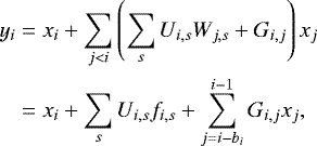
The recursion formulas for the solving (x = L⁻¹y) in the preconditioned case (see Eqs. (34) and (35)) are: $$\begin{array}{l}{\tilde{f}}_{0,s}=0,\\ {\tilde{f}}_{i,s}={\varphi }_{i-1,s}\left({\tilde{f}}_{i-1,s}+{\tilde{W}}_{i-1,s}{x}_{i-1}\right)(i>0),\\ x_i=y_i-{\sum }_s{\tilde{U}}_{i,s}{\tilde{f}}_{i,s}-{\sum }_{j=i-b_i}^{i-1}{G}_{i,j}{x}_j,\end{array}$$

where $\tilde{f}$ is defined such that $$U_{i,s}{f}_{i,s}={\tilde{U}}_{i,s}{\tilde{f}}_{i,s}.$$(A.10)

The case of the dot product is very similar to the above (see Eqs. (36) and (37)) as well as the dot product and solving with L^T.

Appendix B Backpropagation of the gradient for the S + LEAF model

In this section, we explain how to obtain gradient backpropagation algorithms for the S + LEAF model. Foreman-Mackey (2018) provided backpropagation algorithms for the Cholesky decomposition and solving in the case of semiseparable matrices (F = 0 in our notations). We generalize this method to S + LEAF matrices. We do not detail here the full algorithms but we rather describe the method used to obtain them and refer the reader to the reference implementation² for further details.

Let us first recall the steps required to evaluate the log-likelihood (see Sect. 2.1):

• Compute the deterministic part of the model m(θ), and the residuals r = y − m(θ);

• Compute the S + LEAF representation of the covariance matrix A(α), Ũ(α), Ṽ(α), ϕ(α), F(α);

• Compute the Cholesky decomposition of the covariance matrix D, $\tilde{W}$, G;

• Compute the log-determinant ln det(C) = ${\sum }_i$ ln D_i;

• Solve for u = L⁻¹r;

• Compute ${\chi }^2=u^{\text{T}}{D}^{-1}u={\sum }_i\frac{u_i^2}{D_i}$;

• Compute $\ln \mathcal{L}=-\frac{1}{2}\left({\chi }^2+\ln \det (C)+n\ln \det (2\pi )\right)$.

We then need to compute the derivatives $\frac{\partial \ln \mathcal{L}}{\partial \theta }$ and $\frac{\partial \ln \mathcal{L}}{\partial \alpha }$. There are typically two ways to achieve this, the forward and backward propagation of the gradient. In the forward approach, computing the gradient (or the Jacobian matrix) of y_n (x) = f_n○…○f₂○f₁(x) is performed by first computing ∇f₁(x) and propagating it using the relation, $$\nabla y_{k+1}(x)=\nabla f_{k+1}(y_k(x))\nabla y_k(x),$$(B.1)

for k = 1…n − 1. In the backward approach, we first compute ∇f_n(y_n−1(x)), and propagate it using the relation: $$\nabla g_k(y_k(x))=\nabla g_{k+1}(y_{k+1}(x))\nabla f_{k+1}(y_k(x)),$$(B.2)

for k = n − 1…1, with g_k = f_n○…○f_k+1. In both methods, we need to compute the gradient of each function appearing in the composition (each f_i). The relative efficiency of both methods depends on the number of dimension of the parameter space and of the output space. Let us note p the number of parameters, and m_k the number of dimension of y_k (x) = f_k○…○f₂○f₁(x). In the forward approach, each step consists in the computation of a m_k × p matrix as the dot product of a m_k × m_k−1 and a m_k−1 × p matrices. In the backward approach, each step consists of computing a m_n × m_k matrix as the dot product of am_n × m_k+1 and a m_k+1 × m_k matrices (with m₀ = p). Therefore, in the case p < m_n, the forward method should be more efficient, while in the case m_n < p, the backward method should be faster.

In the case of the log-likelihood, we have m_n = 1 (the log-likelihood is a scalar function), and the backward propagation should be preferred. The backpropagation method to compute the gradient of the log-likelihood can be decomposed in the following steps:

• Compute $\frac{\partial \ln \mathcal{L}}{\partial u_i}=-\frac{u_i}{D_i}$;

• Compute $\frac{\partial \ln \mathcal{L}}{\partial D_i}=\frac{1}{2}\left({\left(\frac{u_i}{D_i}\right)}^2-\frac{1}{D_i}\right)$;

• Compute the gradient of $\ln \mathcal{L}$ with respect to Ũ, $\tilde{W}$, ϕ, G, and r by using a backpropagation algorithm for the solving (u = L⁻¹r), and the values of $\frac{\partial \ln \mathcal{L}}{\partial u_i}$;

• Use a backpropagation algorithm for the Cholesky decomposition to compute the gradient of $\ln \mathcal{L}$ with respect to A, Ũ, Ṽ, ϕ, and F;

• Backpropagate the gradient of $\ln \mathcal{L}$ with respect to the residuals to compute $\frac{\partial \ln \mathcal{L}}{\partial \theta }=\frac{\partial \ln \mathcal{L}}{\partial r}\frac{\partial r}{\partial \theta }$;

• Backpropagate the gradient of $\ln \mathcal{L}$ with respect to the S + LEAF decomposition of the covariance to compute $\frac{\partial \ln \mathcal{L}}{\partial \alpha }$.

The kth line of code appearing in the implementation of an algorithm (Cholesky decomposition, dot product y = Lx, solving, etc.) can be seen as a function f_k, while the full code is the composition y_n(x) = f_n○…○f₂○f₁(x). In the case of the Cholesky decomposition, the vector x represents all the entries of A, Ũ, Ṽ, ϕ, and F, while the output y_n(x) represents D, Ũ, $\tilde{W}$, ϕ, and G. The backpropagation of the gradient for the Cholesky decomposition consists in computing the derivatives $\frac{\partial h}{\partial A_i}$, etc., from the values of $\frac{\partial h}{\partial D_i}$, etc., for some function h. Applying the backpropagation method described above (Eq. (B.2)) is equivalent to reading the code of the algorithm in the reverse order (starting from the last line, and reversing the order of each loop) and backpropagating the gradient for each line.

Special care should be taken to ensure the stability of the method. For instance, divisions by zero (or small numbers) should be avoided. The only divisions that appear in the computation of the log-likelihood are the divisions by D_i (in the Cholesky decomposition and in the computation of the χ²) which are unavoidable but not problematic for a well conditioned matrix. In the backpropagation algorithms, we also avoid any division other than divisions by D_i. Let us illustrate why this is preferable with the update formula for the tensor $\tilde{S}$ involved in the Cholesky decomposition algorithm (see Eq. (A.3)). As mentioned in Sect. 2.3.1, when computing the Cholesky decomposition of a S + LEAF matrix, the n × r × r tensor $\tilde{S}$ could be stored in memory as a much smaller r × r matrix and updated in place using Eq. (A.3). Then the final value of this r × r matrix ${\tilde{S}}_{n-1}$ could be used as an initial value in the backpropagation algorithm and updated in place by computing ${\tilde{S}}_{i-1}$ from ${\tilde{S}}_i$ (see Eq. (A.3)), $${\tilde{S}}_{i-1,s,t}=\frac{{\tilde{S}}_{i,s,t}}{{\varphi }_{i-1,s}{\varphi }_{i-1,t}}-{\tilde{W}}_{i-1,s}{D}_{i-1}{\tilde{W}}_{i-1,t}.$$(B.3)

This is done in the celerite code (Foreman-Mackey 2018) as it has a smaller memory footprint. However, looking at the update formula (B.3), we can see that when ϕ_i−1,sϕ_i−1,t ≈ 0, this turns out to be unstable numerically. This issue could thus induce a wrong determination of the gradient, which could slow down or prevent the convergence of minimization algorithms. We thus store the full $\tilde{S}$ tensor in the Cholesky decomposition algorithm, which increases the memory footprint of the algorithm but improves the efficiency and stability of the backpropagation method.

References

All Tables

All Figures

	Fig. 1 Sketch of a symmetric LEAF matrix.
In the text

	Fig. 2 Shapes of the four components of the noise models used for the analysis of the HD 136352 system (Sect. 3).
In the text

Fig. 3 Periodograms of the radial velocity residuals of HD 136352 after subtracting the two first planets (at 11.5824 d and 27.5821 d, left), and after subtracting the three known planets (11.5824 d, 27.5821 d, and 107.6 d right), for the fivenoise models defined in Sect. 3.1. The noise parameters are set to the values provided in Table 1. The vertical blue line highlights the period of the third planet (107.6 d), and the dashed blue lines highlight its aliases at 1 yr. The dotted vertical red lines highlight 0.5 sd, 1 sd, and 1 yr. For the sake of readability, we do not show here the two first periodograms (raw time series and after subtracting the first planet), since the two first planets (11.5824 d and 27.5821 d) are unambiguously detected (highest peaks and FAP < 10−10) independently of the noise model. Assuming that the 107.6 d signal is due to a planet while the signals at 0.5 sd, 1 sd, and around 1 yr are due to correlated noise, we expect the correct noise model to show a low FAP in the left column and a high FAP in the right column.

In the text

References

- Ambikasaran, S. 2015, Numer. Linear Algebra Appl., 22, 1102 [CrossRef] [Google Scholar]
- Baluev, R. V. 2008, MNRAS, 385, 1279 [NASA ADS] [CrossRef] [Google Scholar]
- Byrd, R., Lu, P., Nocedal, J., & Zhu, C. 1995, SIAM J. Sci. Comput., 16, 1190 [Google Scholar]
- Delisle, J.-B., Ségransan, D., Dumusque, X., et al. 2018, A&A, 614, A133 [NASA ADS] [CrossRef] [EDP Sciences] [Google Scholar]
- Delisle, J. B., Hara, N., & Ségransan, D. 2020, A&A, 635, A83 [NASA ADS] [CrossRef] [EDP Sciences] [Google Scholar]
- Dumusque, X., Udry, S., Lovis, C., Santos, N. C., & Monteiro, M. J. P. F. G. 2011, A&A, 525, A140 [NASA ADS] [CrossRef] [EDP Sciences] [Google Scholar]
- Dumusque, X., Pepe, F., Lovis, C., & Latham, D. W. 2015, ApJ, 808, 171 [NASA ADS] [CrossRef] [Google Scholar]
- Faria, J. P., Haywood, R. D., Brewer, B. J., et al. 2016, A&A, 588, A31 [NASA ADS] [CrossRef] [EDP Sciences] [Google Scholar]
- Ferraz-Mello, S. 1981, AJ, 86, 619 [NASA ADS] [CrossRef] [Google Scholar]
- Foreman-Mackey, D. 2018, Res. Notes Am. Astron. Soc., 2, 31 [CrossRef] [Google Scholar]
- Foreman-Mackey, D., Agol, E., Ambikasaran, S., & Angus, R. 2017, AJ, 154, 220 [NASA ADS] [CrossRef] [Google Scholar]
- Hara, N. C., Boué, G., Laskar, J., Delisle, J. B., & Unger, N. 2019, MNRAS, 489, 738 [NASA ADS] [CrossRef] [Google Scholar]
- Haywood, R. D., Collier Cameron, A., Queloz, D., et al. 2014, MNRAS, 443, 2517 [NASA ADS] [CrossRef] [Google Scholar]
- Queloz, D., Henry, G. W., Sivan, J. P., et al. 2001, A&A, 379, 279 [NASA ADS] [CrossRef] [EDP Sciences] [Google Scholar]
- Rajpaul, V., Aigrain, S., Osborne, M. A., Reece, S., & Roberts, S. 2015, MNRAS, 452, 2269 [NASA ADS] [CrossRef] [Google Scholar]
- Rybicki, G. B., & Press, W. H. 1995, Phys. Rev. Lett., 74, 1060 [NASA ADS] [CrossRef] [Google Scholar]
- Schwarzenberg-Czerny, A. 1991, MNRAS, 253, 198 [NASA ADS] [CrossRef] [Google Scholar]
- Udry, S., Dumusque, X., Lovis, C., et al. 2019, A&A, 622, A37 [NASA ADS] [CrossRef] [EDP Sciences] [Google Scholar]
- Vandebril, R., Barel, M. V., Golub, G., & Mastronardi, N. 2005, CALCOLO, 42, 249 [CrossRef] [Google Scholar]
- Zechmeister, M., & Kürster, M. 2009, A&A, 496, 577 [NASA ADS] [CrossRef] [EDP Sciences] [Google Scholar]
Available at https://gitlab.unige.ch/jean-baptiste.delisle/spleaf