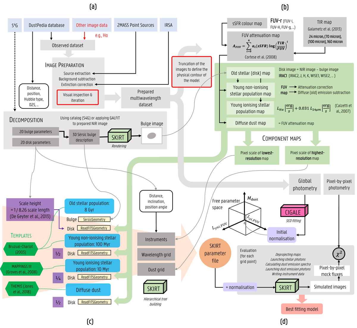
Semi-automatic modelling approach, as implemented in the Python code PTS. Indicated in red are steps that require manual intervention. At the top of the diagram, the different input sources are displayed. These include the DustPedia archive, but also other image data can be included in the modelling environment. The images are prepared uniformly by the pipeline, using the 2MASS point sources catalogue and IRSA service for dust extinction. If Spitzer 3.6 μm or 4.5 μm data is available, a 2D decomposition is retrieved from the S⁴G catalogue; or else custom decomposition parameters can be specified. The prepared images are used to obtain a map of the different stellar and disc components based on well-established prescriptions. What is crucial in the map-making process is the FUV attenuation map which, in turn, is based on an sSFR colour map (the preferential colour is indicated in bold, though other colours can be used depending on the availability and quality of the data) and a TIR map (created by combining multiple MIR/FIR bands with a consideration of the resolution). The maps and 3D bulge description define the geometry of the RT model, together with appropriate scale heights for each of the disc components. The RT model is further defined by a wavelength grid, an instrument setup, and a dust grid. Given this basic model, SKIRT is used to determine the best normalisations of stellar and dust components. For more details, we refer to the main text in Sect. 3. (a) Preparation and decomposition, (b) map making, (c) model construction, and (d) model normalisation (fitting).