| Issue |
A&A
Volume 636, April 2020
|
|
|---|---|---|
| Article Number | A27 | |
| Number of page(s) | 9 | |
| Section | Celestial mechanics and astrometry | |
| DOI | https://doi.org/10.1051/0004-6361/202037446 | |
| Published online | 09 April 2020 | |
An elastic model of Phobos’ libration
1
State Key Laboratory of Information Engineering in Surveying, Mapping and Remote Sensing, Wuhan University, Wuhan 430070, PR China
e-mail: This email address is being protected from spambots. You need JavaScript enabled to view it.
, This email address is being protected from spambots. You need JavaScript enabled to view it.
2
Observatoire géodésique de Tahiti, BP 6570, 98702 Faa’a, Tahiti, French Polynesia, France
Received:
5
January
2020
Accepted:
25
February
2020
Abstract
Context. Study the rotation of a celestial body is an efficient way to infer its interior structure, and then may give information of its origin and evolution. In this study, based on the latest shape model of Phobos from Mars Express (MEX) mission, the polyhedron approximation approach was used to simulate the gravity field of Phobos. Then, the gravity information was combined with the newest geophysical parameters such as GM and k2 to construct the numerical model of Phobos’ rotation. And with an appropriate angles transformation, we got the librational series respect to Martian mean equator of date.
Aims. The purpose of this paper is to develop a numerical model of Phobos’ rotational motion that includes the elastic properties of Phobos. The frequencies analysis of the librational angles calculated from the numerical integration results emphasize the relationship between geophysical properties and dynamics of Phobos. This work will also be useful for a future space mission dedicated to Phobos.
Methods. Based on the latest shape model of Phobos from MEX mission, we firstly modeled the gravity field of Phobos, then the gravity coefficients were combined with some of the newest geophysical parameters to simulate the rotational motion of Phobos. To investigate how the elastic properties of Phobos affect its librational motion, we adopted various k2 into our numerical integration. Then the analysis was performed by iterating a frequency analysis and linear least-squares fit of Phobos’ physical librations. From this analysis, we identified the influence of k2 on the largest librational amplitude and its phase.
Results. We showed the first ten periods of the librational angles and found that they agree well with the previous numerical results which Phobos was treated as a perfectly rigid body. We also found that the maximum amplitudes of the three parameters of libration are also close to the results from a rigid model, which is mainly due to the inclination of Phobos and moments of inertia. The other amplitudes are slightly different, since the physics contained in our model is different to that of a previous study, specifically, the different low-degree gravity coefficients and ephemeris. The libration in longitude τ has the same quadratic term with previous numerical study, which is consistent with the secular acceleration of Phobos falling onto Mars. We investigated the influence of the tidal Love number k2 on Phobos’ rotation and found a detectable amplitude changes (0.0005°) expected in the future space mission on τ, which provided a potential possibility to constrain the k2 of Phobos by observing its rotation. We also studied the influence of Phobos’ orbit accuracy on its libration and suggested a simultaneous integration of orbit and rotation in future work.
Key words: methods: data analysis / celestial mechanics / astrometry / methods: numerical / ephemerides / planets and satellites: dynamical evolution and stability
© ESO 2020
1. Introduction
As one of the two Martian natural moons, Phobos has been an important exploration objective since the very beginning of Mars exploration. The first approximation of its rotational motion was determined by Duxbury & Callahan (1981) using the photographs provided by the Viking orbiter. Considering that the study of a celestial body’s rotation can give access to vital information about its interior structure, such a technique has already been used successfully to infer the interior properties of, for example, the Moon, Mercury, and Earth (Margot et al. 2007; Mathews et al. 2002; Williams et al. 2001). It makes researchers pay a lot of attention to the study of the rotation of Phobos (Rambaux et al. 2012; Pesek 1991; Chapront-Touzé 1990; Borderies & Yoder 1990).
Like the Moon goes around the Earth in a synchronous rotation state, Phobos is in synchronous spin-orbit resonance around Mars. According to the previous understanding of Phobos, similar to the Moon, its rotational motion also deviates from Cassini’s law known as the physical libration. This phenomenon describes Phobos’ oscillation during the rotation, it is a key to studying the rotation of Phobos. Willner et al. (2010) expanded the control points of Phobos by analyzing the image data obtained by the super resolution channel (SRC) on board the European Mars Express (MEX) mission. In addition to the shape model, these researchers derived the amplitude of Phobos’ forced libration at 1.24°. Recently, Willner et al. (2014) updated Phobos’ control points set with the new high super resolution channel (HSRC) images from MEX project, and gave a new estimate for the forced libration amplitude of Phobos with 1.14°. These values deduced from the shape model are not only highly consistent with each other, but also in agreement with the value of 1.03° from the orbital motion of Phobos by Jacobson (2010).
The behavior of Phobos’ physical librations can be mainly explored in two typical schemes: one method is to study through semi-analytical theory. In order to support the Phobos exploration project called Phobos 2, implemented by Russia in 1990s, Pesek (1991), Chapront-Touzé (1990), and Borderies & Yoder (1990) developed analytical theories and computed the physical librations of Phobos. The moment of inertia derived from the analysis of the Viking images by Duxbury (1989) were used, and a Phobos analytical orbital ephemeris called ESAPHO created by Chapront-Touzé (1988) was employed in their elegant studies.
The other approach to study the physical librations of Phobos is based on a purely numerical method. Using a set of numerically integrated dynamical equations and the knowledge of Phobos’ gravity deduced from the shape model, we are able to simulate the rotation of Phobos around Mars. Compared to the semi-analytical one, numerical integration is a more flexible strategy on account of the nonlinear or generally ignored effects during the theoretical analysis. Rambaux et al. (2012) firstly developed a numerical approach to investigate Phobos’ physical librations. In their work, Phobos was treated as an ideally rigid body, the degree of its harmonics coefficients was truncated at three, and also contained the effect of Mars’ oblateness.
Motivated by the latest results on the internal structure of Phobos (Le Maistre et al. 2013, 2019), we developed a new numerical model of Phobos’ rotation that regards Phobos as an elastic body, considering the deformation of Phobos during its motion around Mars. This model enables us to simulate the physical librations of Phobos with a more realistic case. We first describe the modeling framework of Phobos’ rotation and compute the physical librations in Sect. 2. Section 3 presents the physical librations of an elastic Phobos, shows how the amplitude of the primary term libration responses to the tidal deformation parameter k2, and compares the effects of the newest numerical ephemeris with an error on amplitudes of the librational angles. We briefly discuss the results of this paper and gather the main results and conclusions of the paper in Sect. 4.
2. Modeling framework
To numerically analyze the physical libration of Phobos, we first introduce the modeling process in this work. We present the model by dividing the inputs: geophysical parameters, orbital motion, and rotational motion.
2.1. Geophysical model
The gravity field is represented as a spherical harmonic expansion with normalized coefficients ( ,
,  ), and is given by (Kaula 1966):
![Mathematical equation: $$ \begin{aligned} \begin{split}&U(r, \delta , \lambda ) = \frac{\mathrm{GM}}{r} \times \sum _{l=0}^{l_{\max }}{\left(\frac{R_{\rm Pho}}{r}\right)^{l}} \\&\qquad \ \ \qquad \times \sum _{m=0}^{l}\bar{P}_{lm}{(\sin \delta )}[\bar{C}_{lm}\cos m\lambda + \bar{S}_{lm}\sin m\lambda ], \end{split} \end{aligned} $$](/articles/aa/full_html/2020/04/aa37446-20/aa37446-20-eq3.gif) (1)
(1)
where GM is the gravitational constant times the mass of Phobos, l is the degree, m is the order,  are the fully normalized Legendre polynomials, RPho is the reference radius of Phobos, and (r, ϕlat, λ) (where ϕlat for the latitude to distinguish from libration angle ϕ below) are the radius, latitude and longitude in body-fixed coordinates of Phobos, respectively. The spherical coefficients are fully normalized and are related to the unnormalized coefficients as in (Kaula 1966):
 (2)
(2)
where the δ0m is the Kronecker Delta. The corresponding normalized Legendre polynomials  are thus related to the unnormalized polynomials Plm by
  .
.
During the MEX mission, the highly elliptical near polar orbit allowed several close flybys of Phobos every five months (Witasse et al. 2014; Pätzold et al. 2016). This makes it possible to investigate the geophysical parameters of Phobos such as GM and gravity field coefficients  and
and  (Pätzold et al. 2014a). Andert et al. (2010) and Pätzold et al. (2014b) processed the 2006, 2008, and 2010 MEX flyby data and gave a high-precision value of GM for Phobos at (0.7072 ± 0.0013) × 10−3 km3 s−2. However, the second degree gravity field of Phobos (C20, C22) could not be solved for at sufficient accuracy (Pätzold et al. 2014b; Yang et al. 2019a).
In order to determine Phobos’ gravity field coefficients and moment of inertia, which are crucial values in the rotational motion of Phobos, a recently determined precise shape model with 100 m/pixel resolution (Willner et al. 2014) was used to compute its gravity field and moment of inertia. Under the assumption that Phobos has a homogeneous interior, we employed the polyhedron approximation approach (PAA) (Shi et al. 2012; Werner & Scheeres 1996) to calculate the gravity filed of Phobos up to degree 80 (Guo et al., in prep.). The volume of Phobos computed by Willner et al. (2014) is (5.741 ± 0.035) × 103 km3, from the volume and GM of Phobos the average density ρp is calculated to be 1.845 ± 0.012 g cm−3. During the computation, we rotated the reference coordinate system of the shape model into the principal axis frame. Moreover, We used R = 14.0 km instead of 10.993 km (Willner et al. 2014) as the reference radius to compute the gravity field of Phobos. The normalized spherical coefficient C20 value is −0.029395 ± 0.00024, and C22 value is 0.015254 ± 0.00055, consistent with the values developed by Le Maistre et al. (2019) (discrepancy is less than 2%). However, in the calculation below, only the gravity coefficients up to degree eight are used. We found that the integration result no longer changes with higher degrees under current double precision condition. Therefore, the gravity model is truncated at the eighth degree in this work (see Appendix A).
On the other hand, the librational motion has a close relationship with the moment of inertia defined as A, B, and C (A ≤ B ≤ C), which are the principal moments of inertia of Phobos. Specifically, the amplitude of the librational motion in longitude of Phobos depends on the relative moment of inertia γ, where  . According to Chao & Rubincam (1989):
 (3)
(3)
where e = 0.01511 (Jacobson 2010) is the orbital eccentricity of Phobos. To compute the libration, we derived the A, B, and C from the shape model of Phobos with values of 0.355447 ± 0.000011, 0.418102 ± 0.000056, 0.491336 ± 0.000013, which are consistent with the results of Le Maistre et al. (2019) (0.5% discrepancy). The amplitude of the libration is 1.073° ±0.034°.
2.2. Model of Phobos’ orbit
In general, for a celestial body in synchronous spin-orbit resonance around its central body, like the Moon around the Earth, the rotation of the body is strongly coupled with its orbital motion. In this state of motion, any deviation from uniform orbital motion affects the rotational motion immediately, and vice versa. For this reason, the orbital motion and rotational motion of the Moon is usually integrated simultaneously (Folkner et al. 2008, 2014; Viswanathan et al. 2017; Yang et al. 2018). However, due to a lack of observational data of Phobos, the orbital perturbations have only been deliberated in Chapront-Touzé (1990), and Phobos’ rotation rate is set to match the orbit’s mean longitude rate (synchronous rotation) in generating Phobos’s numerical ephemerides (Lainey et al. 2007, 2016; Jacobson 2010). For the first time, Rambaux et al. (2012) established a rotation model of rigid Phobos. To study the physical librations numerically, the numerical ephemerides (Lainey et al. 2007) were employed to provide the relative distance between Phobos and Mars during their analysis. In this study, we used a revised ephemerides of Martian moons developed by Lainey et al. (2016) in our computation. Compared with the previous ephemeris, the accuracy has increased from one kilometer to about 200 m (Yan et al. 2018). The reference frame of the numerical ephemeris is connected to J2000.0.
2.3. Model of Phobos’ rotation
In this work, our numerical model is described by Euler’s rotational equations, which are also often used in investigating the rotation of the terrestrial planets such as the Moon and Mars (Van Hoolst 2010). We adopted a right-handed body-fixed coordinates system with its origin at Phobos’ center of mass and its axes aligned along Phobos’ principal axes of inertia. We used an inertial coordinate system as our fundamental reference. The angular velocity ω, which describes the relation between the principle axis system and inertia system is defined by three angles ϕ, θ, and ψ, which are the Euler angles. A classical sequence Z–X–Z of rotation angles describes the transformation of the two systems. The Euler angle ϕ is the angle along the inertial plane, θ is the angle between the inertial plane and Phobos’ equator plane, meaning the precession and nutation angle, respectively, and ψ is the rotation angle along Phobos’ equator plane. The components of the angular velocity vector ω in the principal axes (PA) system can be described by Euler angles (Goldstein 2011).
 (4)
(4)
Through the Euler equation of rotation, the angular velocity ω depends on the total torques Γ from external bodies. The relation governing the rate of change of angular momentum of a body in an inertial coordinate system can be written succinctly as:
 (5)
(5)
where I represents the moment of inertia tensor, Γ is the torques from external bodies, and t is time. But, in a frame rotating at angular velocity ω, the equation should be written in the following form (where “×” = cross product):
 (6)
(6)
Combined, the mathematical relationship (Eq. (4)) between ω and Euler angles together with physical law (Eq. (5): theorem of angular momentum) we can construct the numerical rotational model of Phobos. In these formulas, the key question lies in modeling the inertia tensor I and total torques Γ from external bodies.
In Rambaux’s (2012) paper, Phobos was treated as a perfectly rigid body. Since the numerical equations are constructed in a reference frame tied to the body and defined by the orientation of the principal moment of inertia. In that situation, the moment of inertia is a diagonal matrix with diagonal elements A, B, and C (defined above). However, this is not the end of the story. In reality, the elastic properties of the material that make up Phobos will react to its spin and tidal potential induced by Mars. Consequently, the moment of inertia of Phobos will change and not keep in diagonal form due to its elastic properties.
In order to study the influence of the elastic properties of Phobos on its rotational motion, we referred to strategy on the Moon by Williams et al. (2001) for full descriptions to construct the equation of Phobos’ rotation. The moment of inertia is spilt into three parts: a fixed part for rigid, a part for tidal deformation due to the attraction of Mars, and a part for spin distortion:
 (7)
(7)
where
![Mathematical equation: $$ \begin{aligned} I_{\rm rigid} = \left[ \begin{matrix} A&0&0\\ 0&B&0\\ 0&0&C \end{matrix} \right], \end{aligned} $$](/articles/aa/full_html/2020/04/aa37446-20/aa37446-20-eq16.gif) (8)
(8)
for the tidal part of the moment, the nine elements of the matrix (indices i, j) are
 (9)
(9)
for the tide-raising body (Mars), M is the mass, and r is Phobos-centered position vector (u is the unit vector, components ui), R is the radius of Phobos, k2 is the second degree Love potential number of Phobos, and δij is Kronecker delta function, which modifies the diagonal components.
As the elastic body will be also distorted from a rotation, which in turn causes a change in the moment of inertia,
![Mathematical equation: $$ \begin{aligned} I_{\rm spin} = \frac{R^5}{3G}\left[ k_2 \left( \omega _i \omega _j - \frac{\omega ^2}{3} \delta _{ij} \right) +s \omega ^2 \delta _{ij} \right]. \end{aligned} $$](/articles/aa/full_html/2020/04/aa37446-20/aa37446-20-eq18.gif) (10)
(10)
The angular velocity vector is ω (components ωi) and the spherical parameters s usually takes values  ,
,  and
and  , respectively (Williams et al. 2001), where n is the mean motion of Phobos.
The torques Γ acting on the rotational motion of Phobos are generally split into two groups: the gravitational interaction of Phobos’ figure with external point-mass (body) and a torque from Mars’ oblateness (J2) to Phobos’ figure, namely, the figure–point mass torque and figure–figure torque.
 (11)
(11)
The torque from a single point mass A acting upon Phobos figure is given as:
 (12)
(12)
where MPho is the mass of Phobos, rpmA is the position of the point mass relative to Phobos, and U is the gravitational potential. Torques are computed for the dynamical figure of Phobos interacting with Mars, Deimos, the Sun, Jupiter, Saturn, and the Earth–Moon system.
The Mars-figure torque is originally referred to in the study of the Moon by Breedlove (1977). This torque results from the interaction of the second zonal harmonic of gravity field of Mars with the gravity field of Phobos. The force acting on a Phobos’ mass element is fdm, where f is Phobos’ potential and is expanded at the second degree of Mars’ gravity filed. The contribution of this element to Phobos’ center of mass (CoM) is dΓ = r × fdm, where r ≡ (r1, r2, r3) is the vector from the CoM to the element. Thus, the total Mars-figure torque is computed by integrating dΓ over the entire mass distribution of Phobos:
 (13)
(13)
Given the zonal gravity coefficients of Mars varying with time, due to the seasonal evaporation and sublimation of the polar ice caps over the Mars year (Konopliv et al. 2006), we used a periodic term given by Konopliv et al. (2011) to get the value of J2.
Therefore, the complete numerical equation of the rotational motion for Phobos is then given as:
![Mathematical equation: $$ \begin{aligned} \frac{\mathrm{d}{{\omega }} }{\mathrm{d}t}= \mathbf I ^\mathbf{-1 }\times \left[ \sum _{i} \mathbf \Gamma _{\text{ fig}{\rm -}\text{pm}} + \mathbf \Gamma _{\text{ fig}{\rm -}\text{fig}} - \frac{\mathrm{d}\mathbf I }{\mathrm{d}t} {\omega } - \mathbf \omega \times \mathbf I {\omega } \right]. \end{aligned} $$](/articles/aa/full_html/2020/04/aa37446-20/aa37446-20-eq25.gif) (14)
(14)
We list the key parameters of our model in Table 1.
Parameters in our numerical model.
3. Physical libration
In this section, the librational motion of Phobos is obtained by integrating the numerical model established in Sect. 2. Then, we thoroughly analyze the influence of tidal deformation parameter k2 and orbital ephemeris on the librational spectrum.
3.1. Introduction
The physical librations are small and are extracted from the three Euler angles describing the orientation and spin rotation of Phobos. The three Euler angles (ϕ, θ, ψ) express the transformation between the inertial reference frame and the principal axis (PA) frame. However, the libration angles designated by Iσ, ρ, and τ (Eckhardt 1981), which describe the small corrections to Cassini’s law of Phobos, are defined with respect to the Martian mean equator of date, but not the inertial frame. Thus, the Euler angles (ϕ, θ, ψ) expressed in the inertial reference system are transformed into the Euler angles (ϕc, θc, ψc) expressed with respect to the Martian mean equator of date by applying the appropriate rotation matrices (Rambaux et al. 2012). The libration angles are defined as:
 (15)
(15)
where Ω denotes the mean longitude of the ascending node of Phobos’ orbit, I represents the constant tilt of Phobos’ equator and λ Phobos’ mean longitude. (Iσ, ρ, τ) are components of physical librations in node, inclination, and longitude, respectively. In practice, the first two components are also well described by using the two components of the unit vector (P1, P2). The direction points towards the mean pole of the Martian mean equator of date on Phobos’ equatorial plane and is defined as:
 (16)
(16)
which make the integration of the theoretical equations of motion easier and are often described in the analytical theories (Petrova 1996; Pesek 1991; Chapront-Touzé 1990). In this paper, based on the previous studies (Eckhardt 1981; Petrova 1996; Rambaux & Williams 2011; Rambaux et al. 2012; Yang et al. 2017), we used P1, P2, and τ to describe the librational motion of Phobos.
3.2. Determination of the free libration
Following the analysis of Eckhardt (1981), by applying a linear operator ℒ on Eq. (6), a linearized equation governing the rotation of the spin-orbit resonant Phobos can be written at the first order as:
 (17)
(17)
here ℱ is the torque, X ≡ [P1, P2, τ]T, and ℒ is the linear operator which can be written as:
![Mathematical equation: $$ \begin{aligned} \left[ \begin{matrix} -\frac{\mathrm{d}^2}{\mathrm{d}t^2} - 4\beta n^2&n(1-\beta )\frac{\mathrm{d}}{\mathrm{d}t}&0\\ n(1-\alpha ) \frac{\mathrm{d}}{\mathrm{d}t}&\alpha n^2 + \frac{\mathrm{d}^2}{\mathrm{d}t^2}&0\\ 0&0&\frac{\mathrm{d}^2}{\mathrm{d}t^2} + 3\gamma \end{matrix} \right], \end{aligned} $$](/articles/aa/full_html/2020/04/aa37446-20/aa37446-20-eq30.gif) (18)
(18)
where  and
and  are the relative moment of inertia. The frequency approximations of the free librations can be obtained from the eigenfrequencies of the ℒ. Thus, the fP1, fP2 are two positive roots of
 (19)
(19)
and
 (20)
(20)
The frequencies fP1, fP2, and fτ correspond to the latitude, wobble, and longitude of the rotation of Phobos, respectively. Based on different results of moment of inertia (Le Maistre et al. 2019; Willner et al. 2014, 2010), approximate values for free modes are listed in Table 2.
Numerical values of Phobos’ free libration modes from moment of inertia.
3.3. Forced librations
To investigate the librations of Phobos numerically, we integrated the numerical equations via single-step Runge–Kutta–Fehlberg (RKF) and multi-steps Adams–Bashforth–Moulton (ABM) (Yang et al. 2018), the integration step is set at 1/24 day (1 h). The initial values of Phobos’ rotation are quoted from Archinal & Acton (2018). However, for a spin-orbit resonant system, the inconsistency between the initial orbital and rotational conditions will generate the excitation of the free modes of libration. To remove the influence of the free libration, we adopted the method proposed by Rambaux et al. (2012) to find the consistent initial condition. The numerical integration is to be performed over 100 years. Figure 1 shows the evolution of the Euler angles defined with respect to the inertial reference frame system over 100 years from 1 Jan 2000 to 2100.
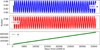 |
Fig. 1. Temporal evolution of Phobos’ Euler angles over about 100 years. |
The libration angles are defined with respect to the Martian mean equator of date and not the inertial reference system as in our numerical results. Thus, we transformed the Euler angles expressed in the inertial reference system to those expressed in the Martian mean equator of date by applying the successive rotation matrices given in Chapront-Touzé (1990). Figures 2 and 3 show the polar coordinates and libration angles, respectively. As shown in Fig. 3, the first librational amplitudes dominating the three curves are nearly 0.02 rad. This value agrees well with the amplitude given by Eq. (3). The (P1, P2) coordinates are plotted in Fig. 2. Its amplitude is equal to about 250 m at the surface of Phobos (using the longest axis of Phobos oriented towards Mars, equal to 13.0 km, Willner et al. 2014).
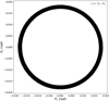 |
Fig. 2. Temporal evolution of latitudinal librations over about 3 years. |
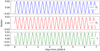 |
Fig. 3. Temporal evolution of libration parameters in 7 days. |
If Phobos followed Cassini’s laws perfectly, the libration in inclination ρ in Eq. (15) would be zero, and the obliquity angle I is expected to be a constant. Here, we fit the θc with a linear function and get the I equal to about 1.0774°, the evolution of the librational angle ρ is plotted in Fig. 4. It indicates that the tilt of the mean equator of Phobos to the Martian equator of date has an oscillating amplitude of 75 arcsec.
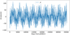 |
Fig. 4. Temporal evolution of libration angle ρ. |
3.4. The fitting method
To estimate the components of the libration parameters P1, P2, and τ, a frequency analysis algorithm and fitting model are needed. We employ the method used in Yang et al. (2017, 2019b) and assume that the solutions of the three quantities have a mathematical form,
![Mathematical equation: $$ \begin{aligned} \begin{split} \mathrm{libr}(t) = \sum _{i = 0}^{3}{a_i t^i} + \sum _{j = 1}^{n} (1 + \mu _j t) \left[C_j \cos (\omega _j t) + S_j \sin (\omega _j t) \right], \end{split} \end{aligned} $$](/articles/aa/full_html/2020/04/aa37446-20/aa37446-20-eq35.gif) (21)
(21)
where ai are the polynomial coefficients, Poisson terms μj are introduced to allow for a time-varying amplitude, ωj are the frequencies, and Cj, Sj are the Fourier series coefficients. All the coefficients < were estimated using a least-squares method.
The physical librations in latitude are described through the pole position with respect to the Martian mean equator of date. We applied the frequency analysis for P1 and P2 to characterize the main librations. Tables 3 and 4 list the periods, amplitudes and phases of the first 10 physical libration spectrums for P1 and P2. These terms are sorted by decreasing amplitude. We also used the analytical description by Chapront-Touzé (1990) to identify the origin of each libration, who provided a constructive description of the orbit of Phobos using Delaunay arguments (l, l′, D, F) in the mean Martian equator of date. These parameters were introduced in detail by Rambaux et al. (2012), and we used the results directly here. The biggest libration is related to the latitudinal argument F that corresponds to the draconic month. This spectrum has an amplitude of 1.0789° and 1.0785° for P1 and P2, respectively. These values are consistent with the equatorial inclination of Phobos. Moreover, the periods of 0.23137 days, 0.84383 days, and 0.84211 days are estimated to be stimulated by the proximity of free modes.
Frequency analysis for P1.
Frequency analysis for P2.
When fitting the angle of libration τ, we found the quadratic coefficient a2 = 0.001276 deg year−2, which is the same value of Rambaux et al. (2012), corresponding to the secular acceleration of Phobos’ orbital motion around Mars. A coupling phenomenon is observed, although the orbital and rotational motion are not simulated simultaneously. The list of librations is detailed below and shown in Table 5. The maximum librational amplitude of τ due to the nonzero eccentricity of Phobos’ orbit is more than one hundred times larger than that of the second spectrum. The amplitude 1.1248° agrees with the value given in Eq. (3) based on the values of moment of inertia. The last term (12.2408 days) of Table 5 is close to the free libration of τ, which may help to constrain the interior structure of Phobos in future (Rambaux et al. 2012).
Frequency analysis for τ.
3.5. Tidal Love number k2
There is still uncertainty about the internal structure of Phobos. In this work, Phobos was treated as an elastic body to construct the numerical model of rotational motion. Consequently, the tidal and spin deformations will affect the rotational motion of Phobos. There are both elastic and dissipation effects. Williams et al. (2001) gave an analytical approximation of how the tidal dissipation influences the librational motion of the Moon. Therefore, to examine the effect of different k2 on Phobos’ rotation, we used various k2 to compute Phobos’ rotation. By considering a range of plausible value for k2 ∈ [10−7, 10−3] (Le Maistre et al. 2013), the largest (main) librational amplitude and its phase of P1, P2, and τ varying with k2, are plotted in Figs. 5, 6 and 7, respectively. As shown in these figures, the shift in the amplitudes of librations are less than 1.0° × 10−6 for P1 and P2, and 0.0005° for τ, respectively. Although the amplitude shifts for P1 and P2 are too small to be detectable, the 0.0005° shift in τ when k2 varies in [10−4, 10−3] is larger than the accuracy expected on geodetic equipment performed with a future landed mission (Le Maistre et al. 2013). In other words, it indicates some potential possibilities to constrain Phobos’ k2 via observing the rotational motion of Phobos with high precision in the future Phobos exploration missions. In this case of Phobos being regarded as an elastic body, there is a time lag between Phobos-Mars direction that will affect the rotation of Phobos, but this factor is not considered in current numerical integration.
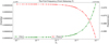 |
Fig. 5. Phobos’ first librational phase (arcsec) and amplitude (deg) of P1 as a function of Love number k2. |
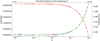 |
Fig. 6. Phobos’ first librational phase (arcsec) and amplitude (deg) of P2 as a function of Love number k2. |
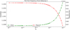 |
Fig. 7. Phobos’ first librational phase (arcsec) and amplitude (deg) of τ as a function of Love number k2. |
3.6. Orbit of Phobos
As pointed out in Sect. 2.2, Phobos’ synchronous spin-orbit resonance state suggests that we should simulate its rotational motion and orbital motion simultaneously. However, due to the lack of high-precision directly observed data, we utilized an independent orbit ephemeris of Phobos in hope of maintaining the accuracies during our numerical computation. Based on the current accuracy of ephemeris, we explore the influence of the ephemeris errors on the rotation of Phobos. Instead of using the past version ephemerides, we added an artificial error directly to the newest ephemeris since we assumed the newest ephemeris has the best accuracy. The error is set as a constant of ±100 m for three directions of x, y, and z in Cartesian coordinates. We subtracted the librational angles containing errors from the those without errors, and then use the mean and root mean square (RMS) of the differences to evaluate its influence on the three librational angles. Tables 6 and 7 present the comparison of the three librational angles using the ephemeris directly and adding a constant error to the ephemeris. The mean differences of P1, P2 and τ in the third case, for example, are 2.743790″, −0.093440″, and −0.000362″, but with RMSs of 0.107513″, 0.086477″, and 0.524639″, respectively. It shows that the P2 is relatively less sensitive to changes in position compared to P1 and τ. Here, we give a semi-analytical explanation of this: frequency analysis shows that the main (first) spectrum of sin θc and sin ψc(cosψc) are exactly the same as 0.3188 days, the phase of period 0.3188 days are fitted as −5.21° and −3.11°, respectively. Thus, we can rewrite them as the following approximations:
 (22)
(22)
where ω0 = 19.7088 rad day−1, ϕ0, (ϕ0 + δϕ) are the phase, and δϕ = 2.1°. Then, the P1 and P2 defined in Eq. (16) can be expressed as:
 (23)
(23)
or, equivalently:
![Mathematical equation: $$ \begin{aligned}&P_1 = \sin ^{2}(\omega _{0}t + \phi _{0}) \cos \delta \phi + \frac{1}{2}\sin [2(\omega _{0}t + \phi _{0})]\sin \delta \phi ,\nonumber \\&P_2 = -\sin ^{2}(\omega _{0}t + \phi _{0}) \sin \delta \phi + \frac{1}{2}\sin [2(\omega _{0}t + \phi _{0})]\cos \delta \phi . \end{aligned} $$](/articles/aa/full_html/2020/04/aa37446-20/aa37446-20-eq38.gif) (24)
(24)
Orbit errors on librational angles of Phobos (mean value).
Orbit errors on librational angles of Phobos (RMS).
Such a recombination of the trigonometric functions indicates the mean value of P1 and P2 have the following relationship:
 (25)
(25)
which agrees well with the value −26.74 calculated directly from the librational series.
Furthermore, we define
 (26)
(26)
where  ,
,  denote the P1 and P2 series containing constant orbit error, δθ and δψ are small. Considering the θc is also small, cosθc is much larger than sin θc. Finally, we retain the main term as:
 (27)
(27)
Similar to Eq. (23), we can conclude the mean difference also satisfy a relationship such as that in Eq. (25), and Table 6 shows the consistency (where ΔP1/ΔP2 ≈ −29) with the analysis. Due to the complex nonlinear expression of τ, it is not analyzed in this work.
4. Discussion and conclusions
The rotation of a celestial body provides remote observers clues as to its interior structure, origins, and evolution. This paper sheds light on the rotation of Phobos’ poorly understood satellite of Mars, by optimizing an existing numerical model to account for elastic properties of Phobos. In contrast to a theoretical model, a numerical model provides an opportunity to explore the nonlinear attributes of rotation, which are usually difficult to consider in theoretical analysis, and computationally efficient. Based on our preliminary analysis, we extended our research to the rotational motion of Phobos to include the librational frequencies, tidal Love number, and the effect of orbit accuracy on our rotation model.
We extracted the first ten librational frequencies sorted by amplitude from our integration results for P1, P2, and τ. The frequencies agree with the rigid body model by Rambaux et al. (2012). Moreover, we also find that the maximum amplitudes of the three parameters are close to the results from rigid model, probably since these are mainly affected by the inclination and the moments of inertia of Phobos. The other amplitudes are slightly different due to the different low-degree gravity coefficients, especially the third degree coefficients (Rambaux et al. 2012) and different ephemeris of Phobos used in calculation.
Mars induces tidal deformation and therefore additional torque on Phobos. Hence, the tidal Love number k2 was taken into account when estimating maximum librational angles. We used a set of values of k2 from 10−7 to 10−3 to explore how the amplitude change of the librational angles. We find that the maximum amplitude changes of P1 and P2 were less than 1.0° × 10−6 and very difficult to detect. When k2 varies from 10−4 to 10−3, the amplitude change for the τ reaches about 0.0005° and at the equal magnitude of precision expected in future mission. Therefore, these results provided a potential method to study the k2 of Phobos by observing its rotation.
To investigate how much the orbit accuracy affects the libration, we added a constant error to the ephemeris of Phobos. A direct comparison indicated that the P2 was relatively less sensitive to the orbit accuracy of Phobos in our test case, relative to P1 and τ. Although our results do not clearly show how the coupling of orbit and rotation affect the rotational motion of Phobos, nevertheless, future high-precision orbit will undoubtedly give more convincing rotation models. A simultaneous integration of orbit and rotation in our future work will also give a clear answer to this problem.
The results of this work provide a useful reference on the numerical study of Phobos’ rotation. In the future, a dedicated geodetic mission to Phobos such as Phobos-Soil and also Martian Moons Exploration (MMX) will help us to take full advantage of the relationship between the interior and dynamics.
Acknowledgments
This research is supported by the National Natural Science Foundation of China (U1831132), Grant of Hubei Province Natural Science (2018CFA087), Open Project of Lunar and Planetary Science Laboratory, Macau University of Science and Technology (FDCT 119/2017/A3). J. P. Barriot is founded by a DAR grant in planetology from the French Space Agency (CNES). Y. Yang thanks Dr. Nicolas Rambaux who kindly provided the analytical results by Chapront-Touzé (1990) and Mr. Xuan Yang on the discussion to utilize the SPICE Toolkit.
References
- Andert, T., Rosenblatt, P., Pätzold, M., et al. 2010, Geophys. Res. Lett., 37, L09202 [NASA ADS] [CrossRef] [Google Scholar]
- Archinal, B., Acton, C., A’Hearn, M., et al. 2018, Mech. Dyn. Astron., 130, 22 [Google Scholar]
- Borderies, N., & Yoder, C. F. 1990, A&A, 233, 235 [NASA ADS] [Google Scholar]
- Breedlove, W. 1977, Scientific Applications of Lunar Laser Ranging (Springer), 65 [NASA ADS] [CrossRef] [Google Scholar]
- Chao, B. F., & Rubincam, D. P. 1989, Geophys. Res. Lett., 16, 859 [NASA ADS] [CrossRef] [Google Scholar]
- Chapront-Touzé, M. 1988, A&A, 200, 255 [NASA ADS] [Google Scholar]
- Chapront-Touzé, M. 1990, A&A, 235, 447 [NASA ADS] [Google Scholar]
- Duxbury, T. C. 1989, Icarus, 78, 169 [NASA ADS] [CrossRef] [Google Scholar]
- Duxbury, T. C., & Callahan, J. D. 1981, AJ, 86, 1722 [NASA ADS] [CrossRef] [Google Scholar]
- Eckhardt, D. H. 1981, Moon Planets, 25, 3 [NASA ADS] [CrossRef] [Google Scholar]
- Folkner, W. M., Williams, J. G., & Boggs, D. H. 2008, IPN Prog. Rep., 42, 178 [Google Scholar]
- Folkner, W. M., Williams, J. G., Boggs, D. H., Park, R. S., & Kuchynka, P. 2014, Interplanet. Network Prog. Rep., 196, 1 [Google Scholar]
- Goldstein, H. 2011, Classical Mechanics (Pearson Education India) [Google Scholar]
- Jacobson, R. 2010, AJ, 139, 668 [Google Scholar]
- Kaula, W. M. 1966, Theory of Satellite Geodesy (Waltham, MA: Blaisdell Publ. Co) [Google Scholar]
- Konopliv, A. S., Yoder, C. F., Standish, E. M., Yuan, D.-N., & Sjogren, W. L. 2006, Icarus, 182, 23 [NASA ADS] [CrossRef] [Google Scholar]
- Konopliv, A. S., Asmar, S. W., Folkner, W. M., et al. 2011, Icarus, 211, 401 [NASA ADS] [CrossRef] [Google Scholar]
- Lainey, V., Dehant, V., & Pätzold, M. 2007, A&A, 465, 1075 [NASA ADS] [CrossRef] [EDP Sciences] [Google Scholar]
- Lainey, V., Pasewaldt, A., Robert, V., et al. 2016, A&A, submitted [Google Scholar]
- Le Maistre, S., Rosenblatt, P., Rambaux, N., et al. 2013, Planet. Space Sci., 85, 106 [NASA ADS] [CrossRef] [Google Scholar]
- Le Maistre, S., Rivoldini, A., & Rosenblatt, P. 2019, Icarus, 321, 272 [NASA ADS] [CrossRef] [Google Scholar]
- Margot, J., Peale, S. J., Jurgens, R. F., Slade, M. A., & Holin, I. V. 2007, Science, 316, 710 [NASA ADS] [CrossRef] [PubMed] [Google Scholar]
- Mathews, P. M., Herring, T. A., & Buffett, B. A. 2002, J. Geophys. Res., 107, ETG-3 [Google Scholar]
- Pätzold, M., Andert, T., Jacobson, R., Rosenblatt, P., & Dehant, V. 2014a, Planet. Space Sci., 102, 86 [NASA ADS] [CrossRef] [Google Scholar]
- Pätzold, M., Andert, T., Tyler, G., et al. 2014b, Icarus, 229, 92 [NASA ADS] [CrossRef] [Google Scholar]
- Pätzold, M., Häusler, B., Tyler, G., et al. 2016, Planet. Space Sci., 127, 44 [NASA ADS] [CrossRef] [Google Scholar]
- Pesek, I. 1991, Bull. Astr. Inst. Czechosl., 42, 271 [NASA ADS] [Google Scholar]
- Petrova, N. 1996, Earth Moon Planets, 73, 71 [NASA ADS] [CrossRef] [Google Scholar]
- Rambaux, N., & Williams, J. 2011, Celest. Mech. Dyn. Astron., 109, 85 [NASA ADS] [CrossRef] [Google Scholar]
- Rambaux, N., Castillo-Rogez, J. C., Maistre, S. L., & Rosenblatt, P. 2012, A&A, 548, A14 [NASA ADS] [CrossRef] [EDP Sciences] [Google Scholar]
- Shi, X., Willner, K., Oberst, J., Ping, J., & Ye, S. 2012, Sci. Chin. Phys. Mech. Astron., 55, 358 [NASA ADS] [CrossRef] [Google Scholar]
- Van Hoolst, T. 2010, Treatise Geophys., 10, 123 [NASA ADS] [CrossRef] [Google Scholar]
- Viswanathan, V., Fienga, A., Gastineau, M., & Laskar, J. 2017, Notes Sci. Inst. Mech. Celest. Tech., 108 [Google Scholar]
- Werner, R. A., & Scheeres, D. J. 1996, Celest. Mech. Dyn. Astron., 65, 313 [NASA ADS] [Google Scholar]
- Williams, J. G., Boggs, D. H., Yoder, C. F., Ratcliff, J. T., & Dickey, J. O. 2001, J. Geophys. Res., 106, 27933 [NASA ADS] [CrossRef] [Google Scholar]
- Willner, K., Oberst, J., Hussmann, H., et al. 2010, Earth Planet. Sci. Lett., 294, 541 [NASA ADS] [CrossRef] [Google Scholar]
- Willner, K., Shi, X., & Oberst, J. 2014, Planet. Space Sci., 102, 51 [NASA ADS] [CrossRef] [Google Scholar]
- Witasse, O., Duxbury, T., Chicarro, A., et al. 2014, Planet. Space Sci., 102, 18 [NASA ADS] [CrossRef] [Google Scholar]
- Yan, J., Yang, X., Ye, M., et al. 2018, MNRAS, 481, 4361 [NASA ADS] [CrossRef] [Google Scholar]
- Yang, Y.-Z., Li, J.-L., Ping, J.-S., & Hanada, H. 2017, Res. Astron. Astrophys., 17, 127 [NASA ADS] [CrossRef] [Google Scholar]
- Yang, Y., Ping, J., Yan, J., & Li, J. 2018, Ap&SS, 363, 190 [NASA ADS] [CrossRef] [Google Scholar]
- Yang, X., Yan, J., Andert, T., et al. 2019a, MNRAS, 490, 2007 [NASA ADS] [CrossRef] [Google Scholar]
- Yang, Y., He, Q., Ping, J., Yan, J., & Zhang, W. 2019b, Ap&SS, 364, 218 [NASA ADS] [CrossRef] [Google Scholar]
Appendix A: Gravity coefficients for a homogeneous Phobos
Table A.1 lists the gravity coefficients for a homogeneous Phobos obtained with the PAA described in Sect. 2 up to degree eight.
Gravity coefficients for a homogeneous Phobos obtained with the PAA described in Sect. 2.
All Tables
Gravity coefficients for a homogeneous Phobos obtained with the PAA described in Sect. 2.
All Figures
|
Fig. 1. Temporal evolution of Phobos’ Euler angles over about 100 years. |
| In the text | |
|
Fig. 2. Temporal evolution of latitudinal librations over about 3 years. |
| In the text | |
|
Fig. 3. Temporal evolution of libration parameters in 7 days. |
| In the text | |
|
Fig. 4. Temporal evolution of libration angle ρ. |
| In the text | |
|
Fig. 5. Phobos’ first librational phase (arcsec) and amplitude (deg) of P1 as a function of Love number k2. |
| In the text | |
|
Fig. 6. Phobos’ first librational phase (arcsec) and amplitude (deg) of P2 as a function of Love number k2. |
| In the text | |
|
Fig. 7. Phobos’ first librational phase (arcsec) and amplitude (deg) of τ as a function of Love number k2. |
| In the text | |
Current usage metrics show cumulative count of Article Views (full-text article views including HTML views, PDF and ePub downloads, according to the available data) and Abstracts Views on Vision4Press platform.
Data correspond to usage on the plateform after 2015. The current usage metrics is available 48-96 hours after online publication and is updated daily on week days.
Initial download of the metrics may take a while.