| Issue |
A&A
Volume 635, March 2020
|
|
|---|---|---|
| Article Number | A180 | |
| Number of page(s) | 14 | |
| Section | Stellar atmospheres | |
| DOI | https://doi.org/10.1051/0004-6361/201937413 | |
| Published online | 31 March 2020 | |
Hydrogen ionization equilibrium in magnetic fields
Instituto de Ciencias Astronómicas, de la Tierra y del Espacio (CONICET),
Av. España 1512 (sur), 5400 San Juan, Argentina
e-mail: rene.rohrmann@conicet.gov.ar
Received:
24
December
2019
Accepted:
10
February
2020
We assess the partition function and ionization degree of magnetized hydrogen atoms at thermodynamic equilibrium for a wide range of field intensities, B ≈ 105–1012 G. Evaluations include fitting formulae for an arbitrary number of binding energies, the coupling between the internal atomic structure and the center-of-mass motion across the magnetic field, and the formation of the so-called decentered states (bound states with the electron shifted from the Coulomb well). Non-ideal gas effects are treated within the occupational probability method. We also present general mathematical expressions for the bound state correspondence between the limits of zero-field and high-field. This let us evaluate the atomic partition function in a continuous way from the Zeeman perturbative regime to very strong fields. Results are shown for conditions found in atmospheres of magnetic white dwarf (MWD) stars, with temperatures T ≈ 5000–80 000 K and densities ρ ≈ 10−12–10−3 g cm3. Our evaluations show a marked reduction of the gas ionization due to the magnetic field in the atmospheres of strong MWDs. We also found that decentered states could be present in the atmospheres of currently known hot MWDs, giving a significant contribution to the partition function in the strongest magnetized atmospheres.
Key words: atomic processes / magnetic fields / stars: atmospheres
© ESO 2020
1 Introduction
The strongest magnetic fields are found in stellar objects, including magnetic white dwarf (MWD) stars with field strengths in a broad range B ≈ 103–109 G, the lower value likely being a result of detection method limits (Ferrario et al. 2015); neutron stars 108–1013 G (Konar 2017); and magnetars, i.e., highly magnetized neutron stars, 1014–1015 G (Harding & Lai 2006; Kaspi & Beloborodov 2017). In comparison, sunspots usually have B≲103 G; Ap- or Bp-type main-sequence stars have 103–104 G; and the strongest stable magnetic fields generated in terrestrial experiments reach about 105 G (Crow et al. 1995), although higher fields (≈107 G) can be produced in magnetic-flux compressions with very short lifetimes τ≲10−7 s (Herlach 1999; Gotchev et al. 2009). Among the mentioned magnetic systems, only magnetars have fields above the critical value Bc = 4.414 × 10¹³ G where the cyclotron energy exceeds the electron rest energy and particle motions become relativistic (Bc is defined by setting ℏωe = mec2, where ωe = eB∕mec is the cyclotron frequency and conventional notation is used).
Most compact stars have hydrogen in the outer layers, mainly because the element segregation in their strong gravitational fields. The structure of atoms is considerably modified in magnetized compact stars beyond the Zeeman-type perturbative approach. These changes have consequences on the internal partition function, energy level populations, ionization equilibrium, and radiative cross-sections, which through the radiative transport give form to the thermal radiation emerging from the stellar surface. The study of atoms in high magnetic field is, therefore, essential for interpretation of emergent spectra from atmospheres and radiating surfaces of compact stars (Külebi et al. 2009; Potekhin 2014). It also has considerable interest for solid state physics (Elliott & Loudon 1960; Orton 2004; Bartnik et al. 2010) and fundamental physics (Friedrich & Wintgen 1989).
The effects of magnetic fields over the atomic structure are usually measured with the parameter β = B∕B0, where B0 ≈ 4.70103 × 10⁹ G is set by equating the Bohr radius (aB = ℏ2∕ mec2) to the characteristic magnetic length  (the mean value of the cyclotron radius in the lowest Landau state). Thus, β ≪ 1 includes the regime of weak magnetic fields, β ≈ 1 the regime where Coulomb and magnetic forces in the atom have comparable strengths, and β ≫ 1 the domain of the magnetic field on particle dynamics transverse to the field direction.
The properties of hydrogen atoms in an external magnetic field have been the subject of investigations over many decades (Garstang 1977; Johnson et al. 1983; Lai 2001; Thirumalai & Heyl 2014). It has already been recognized in studies of excitons (electron–hole pairs) in semiconductors (Elliott & Loudon 1960; Hasegawa & Howard 1961) that, for very strong fields (β ≫ 1), the energy eigenfunctions can be approximated by the product of a Landau orbital (an energy eigenstate corresponding to a free-electron in the field B) and a function depending on the coordinate parallel to the field. This is known as the adiabatic approximation, introduced by Schiff & Snyder (1939), which becomes exact in the limit β →∞, where the behavior of the (non-relativistic) atomic states is reproduced by analytical results based on the one-dimensional hydrogen atom (Loudon 1959, 2016; Haines & Roberts 1969).
Motivated by the discovery of pulsars (β ≳ 1) and magnetic white dwarfs (β≲1), energy evaluations were obtained with variational techniques using trial wavefunctions (Cohen et al. 1970; Smith et al. 1972), followed by more detailed numerical calculations at β ≫ 1 using the adiabatic approximation (e.g., Canuto & Kelly 1972). Corrections to previous results were progressively obtained to reach a comprehensive account of the first low-energy levels from appropriate wavefunction expansions in terms of spherical harmonics (β≲1) or Landau states (β ≳ 1) (Roesner et al. 1984). More recently, some authors (e.g., Kravchenko et al. 1996) found very accurate non-relativistic solutions for a few H states in constant fields of arbitrary strength. Currently, high-precision values are known for a large number of energy states over the whole range of magnetic field strengths using a wavefunction expansion in terms of B-splines (Schimeczek & Wunner 2014).
The above-cited studies assume an infinite nuclear mass and neglect the motion of the atoms. However, astrophysical fluid models require taking finite temperatures and hence the thermal motion of particles into account. Pavlov-Verevkin & Zhilinskii (1980) found simple energy scaling rules to account for the effects of finite proton mass for atoms at rest, but considerations of the particle movement effects are more complex. Motion perpendicular to a magnetic field breaks the axial symmetry that characterizes an atom at rest and makes this problem fully three-dimensional. Gor’kov & Dzyaloshinskii (1968) showed that the motion of an atom across a magnetic field affects its internal energies. They found a conserved quantity, the so-called pseudo-momentum K introduced by Johnson & Lippmann (1949) for single charges, which makes the separation of the center-of-mass (CM) motion from the relative electron-proton motion possible. At large enough values of the pseudo-momentum transverse to the magnetic field (k⊥), or equivalently when a large electric field crosses the magnetic field, the wave function of the relative motion is shifted from the Coulomb center to a magnetic well (Burkova et al. 1976). These states are called decentered states and are characterized by a large dipole moment as a result of the corresponding separation between the electron and proton. Ipatova et al. (1984) showed that the change in the dependence of the atom energy on the pseudo-momentum from centered (the wave function concentrated near the Coulomb well) to decentered states is rather abrupt and occurs when k⊥ reaches a certain critical value  . Perturbative calculations of this dependence at
  were implemented by Vincke & Baye (1988) and Pavlov & Meszaros (1993). Non-perturbative results have been given in different works (Vincke et al. 1992; Lai & Salpeter 1995; Potekhin 1998; Lozovik & Volkov 2004; Potekhin et al. 2014).
The ionization equilibrium of hydrogen in strong magnetic fields was first discussed by Gnedin et al. (1974). Khersonskii (1987a,b) improved on a previous study by taking into account quantization of protons and finite nuclear mass in the atomic internal states. The influence of the pseudo-momentum on the atomic partition function was considered by Ventura et al. (1992), but did not provide quantitative results. Pavlov & Meszaros (1993) included changes of the internal atomic structure caused by the thermal motion of the atoms across the magnetic field, using perturbative evaluations at β ≳ 1. Approximate evaluations of the hydrogen ionization equilibrium including pseudo-momentum effects were considered at Lai & Salpeter (1995) for superstrong fields (β ≫ 1), and improved results were then given by Potekhin and coworkers (e.g., Potekhin et al. 1999, 2014); these results also focused on the very intense magnetic fields of neutron star atmospheres (B ≳ 1010 G).
The aim of the present paper is to evaluate the ionization equilibrium of magnetized hydrogen atoms in the region of intermediate values of magnetic field (mainly B ≈ 105–1010 G), which have remained unexplored so far. For this purpose, we write fitting formulae for the energies of bound states in the transition between field-free and high-field regimes using accurate numerical data for atoms at rest, combined with analytical results of CM effects due to thermal particle motions. On the other hand, we develop mathematical relations to express the correspondence between states in the field-free and strong-field regimes. Our study is focused on conditions found in the atmospheres of magnetic white dwarf stars with megagauss fields (B ≈ 106–109 G), for which zero-field occupation numbers of atoms and ions are currently used (Euchner et al. 2002; Aznar Cuadrado et al. 2004; Külebi et al. 2009).
The paper is organized as follows. Section 2 shows the quantum problem of a hydrogen atom in an uniform magnetic field. Section 3 is devoted to establishing simple rules for the relationships between atomic states in the weak and strong field limits. Section 4 reviews the binding energies of atoms in a magnetic field on different regimes including the treatement of finite nuclear mass and moving particle effects. Section 5 summarizes the chemical potentials, partition function, and ionization equilibrium equations. Results and their analysis are shown in Sect. 6. Concluding remarks are given in Sect. 7.
2 Hydrogen atoms in a magnetic field
The Hamiltonian of the hydrogen atom in a magnetic field omitting relativistic effects is
 (1)
(1)
where qi, mi, ri, pi, and πi are respectively the charge (qe = − e, qp = e), mass, position, canonical momentum, and kinetic momentum of the electron (i = e) or proton (i = p); A is the potential vector of the field and V (r) = − e2∕r the Coulomb potential with r the magnitude of r = re −rp.
For homogeneous magnetic fields B, the motion integral of the atom related with the translational invariance of the Hamiltonian is given by the pseudo-momentum operator K (Gor’kov & Dzyaloshinskii 1968; Avron et al. 1978; Herold et al. 1981; Johnson et al. 1983)
 (3)
(3)
with b = eB∕c and the gauge
 (4)
(4)
Here K is used to separate the relative motion of the electron and proton from the mass center motion (Gor’kov & Dzyaloshinskii 1968). The eigenenergy equation of the atom in relative coordinates can be written in the form (Herold et al. 1981)
![\begin{equation*}\left[\frac{\pi^2}{2\mu} +\frac{(\bm{k}+\bm{b}\,{\times}\,\bm{r})^2}{2M} +V(r) \right]\phi(\bm{r}) =E\phi(\bm{r}), \end{equation*}](/articles/aa/full_html/2020/03/aa37413-19/aa37413-19-eq8.png) (5)
(5)
with ϕ(r) the eigenfunction of Hamiltonian and
 (6)
(6)
k being an eigenvalue of the pseudo-momentum operator K, p the one-particle canonical momentum (p = − iℏ∇r in the relative coordinate space), M the total mass, μ the reduced mass, and γ a relative mass difference,
 (7)
(7)
Equation (5) has been largely studied for atoms at rest (k = 0), where the Hamiltonian of the relative motion of electron and proton takes the form
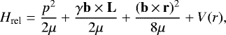 (8)
(8)
L = r × p being the relative angular momentum operator.
Hereafter, we adopt the z-axis of the Cartesian and cylindrical coordinates oriented in the B direction.
States in the zero- and strong-field limits
A brief review of atomic states in the limits β → 0, ∞ is required to specify the correspondence between them. When the magnetic field is switch off, Eq. (8) reduces to the Hamiltonian of the usual Coulomb problem. Bound states are typically represented by eigenstates ϕn,l,m common to the Hamiltonian, L2, and Lz operators, which have eigenvalues − EH∕n2, ℏ2 l(l + 1), and ℏm, respectively, depending on the principal (n = 1, 2, …), orbital (l = 0, 1, …, n − 1), and magnetic (m = − l, …, l − 1, l) quantum numbers, where EH = 13.605693 eV is the ionization energy of the field-free atom.
At very intense field values (β ≫ 1) Coulomb interaction has a negligible effect on the (electron and proton) relative motion transverse to the magnetic field. Eigenfunctions of Hrel can then be factorized in the product (Schiff & Snyder 1939) as
 (9)
(9)
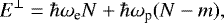
with separated dependence on cylindrical coordinates (r⊥, φ, z), while the eigenenergies are expressed as a sum:
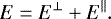 (10)
(10)
Due to the presence of the magnetic field L2 is no longer a conserved quantity, but the Hamiltonian still commutes with Lz, and m thus remains a good quantum number. The transversal part of the eigenfunction is given by the usual Landau function  labeled m and the Landau number N, while the longitudinal component
  of the wavefunction is determined by an effective potential parallel to the field, with ν the longitudinal quantum number which takes non-negative integer values for negative values of E∥ (in this case, ν gives the number of nodes of
  ) and is continuous otherwise.
With the zero-point and spin terms subtracted, the transverse contribution to the eigenenergy in Eq. (10) can be written as
 (11)
(11)

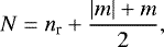
nr (= 0, 1, 2, …) being the radial quantum number which enumerates the nodes of  along the coordinate r⊥. Because nr ≥ 0 and m ≤ N (= 0, 1, 2, …), E⊥ is positive or zero.
Binding values of the longitudinal energy (E∥ < 0) exist for m ≤ 0 and were calculated with the one-dimensional hydrogen atom approach (Loudon 1959; Haines & Roberts 1969). Its solutions are composed by tightly bound states (ν = 0) and hydrogen-like states (ν = 1, 2, 3…). The longitudinal energies of tightly bound states can be approximated by (Ruderman 1974)
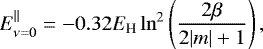 (14)
(14)
while those of hydrogen-like states converge to a Rydberg series
![\begin{equation*}E^{\parallel}_{\nu>0}=-E_{\text{H}} \left[\text{Int} \left(\frac{\nu+1}2\right) + \delta_{\nu m}\right]^{-2}, \end{equation*}](/articles/aa/full_html/2020/03/aa37413-19/aa37413-19-eq22.png) (15)
(15)
with Int(x) the integer part of x, and δνm a quantum defect parameter which takes negative values and vanishes in β →∞ (Friedrich & Wintgen 1989), e.g.,  .
.
Solutions (14) and (15) correspond to a fixed Coulomb potential (i.e., infinitely massive proton). If finite nuclear-mass effects are ignored, the only bound states below the first Landau level (N = 0) are those with m ≤ 0 (nr = 0). States over the first Landau level, which determines the edge of the continuum energy, are metastable (m < N, nr > 0) or truly bound (m = N, nr = 0) depending on the existence or not of lower states with the same magnetic quantum number (Simola & Virtamo 1978). When the finite proton mass is taking into account only states with N = 0 and m = 0 remain below the continuum edge at β →∞ (see Eq. (25)).
3 Bound state correspondence
At very weak magnetic fields (β ≪ 1) the atomic states are well described by the Coulomb quantum numbers {n, l, m}. The Zeeman quadratic effect removes the l degeneracy of low-lying states in β≲10−3, while n remains a good quantum number. Inter-n mixing starts to appear at highly excited states for very low fields and reaches the lowest states at β ≈ 1. In the n mixing regime, the energy level pattern is characterized by many close anti-crossings (Ruder et al. 1994; Schimeczek & Wunner 2014). This complex structure disappears for strong magnetic fields (β ≫ 1) where a newordered structure arises formed by Rydberg-like levels plus tightly bound states. There the set of quantum numbers {N, ν, m} becomes appropriate to describe the atomic states. Two quantities are conserved over the whole range of magnetic fields, the z-parity (πz) of the energy eigenfunctions and the z-component of the orbital angular momentum (quantum number m). Consequently, πz and m remain as good quantum numbers in arbitrary field intensity. As is well-known, the longitudinal parity is  for free-field states and
  for bound states in the strong field regime.
The correspondence between energy states at low and high fields was clarified by Simola & Virtamo (1978) using the non-crossing rule of states. With this rule, which applies to states with exactly the same symmetries on the Hamiltonian operator, bound states in both limits (β → 0, ∞) corresponding to the same πz and m are connected on the order of growing energy. Nevertheless, there are (N, ν, m) states that remain at β → 0 as a linear combinationof two or more (n, l, m) states with the same n and m but different l, one of these states usually being the dominant one. In practice, for degenerate (n, m, πz) multiplets we can adopt the state with highest l which has the lowest energy at β ≪ 1 (Ruder et al. 1994). Adopting this convention, it is possible to establish a complete one-to-one correspondence between the field-free states and strong-field states.
Following the previous convention, we found simple relationships connecting the sets of quantum numbers of bound states in field-free and high-intensity field regimes. In particular, we can express ν in terms of Coulomb quantum numbers in a straightforward way. For states with positive parity πz = + 1, i.e., even (l + m) and even ν,
Longitudinal quantum number ν of high-field states connected to zero-field states (n, l, m) for levels 1 ≤ n ≤ 5 and n = 20.
![\begin{equation*}\nu =\left\{ \begin{array}{@{}ll}\displaystyle \frac{1}{2}\left[(n-|m|+1)^2-4\right]-l+|m|, &\quad \text{odd}~(n+m), \\ [2ex]\displaystyle \frac{1}{2}\left[(n-|m|+1)^2-5\right]-l+|m|, &\quad \text{even}~(n+m).\\ \end{array} \right. \end{equation*}](/articles/aa/full_html/2020/03/aa37413-19/aa37413-19-eq26.png) (16)
(16)
For states with negative parity πz = − 1, i.e., odd (l + m) and odd ν,
![\begin{equation*}\nu = \left\{ \begin{array}{@{}ll}\displaystyle \frac{1}{2}\left[(n-|m|)^2-1\right]-l+|m|, &\quad \text{odd}~(n+m), \\ [2ex]\displaystyle \frac{1}{2}(n-|m|)^2-l+|m|, &\quad \text{even}~(n+m).\\ \end{array} \right. \end{equation*}](/articles/aa/full_html/2020/03/aa37413-19/aa37413-19-eq27.png) (17)
(17)
The correlation between bound states is closed with the relation
 (18)
(18)
Equations (16)–(18) give a complete correspondence between (n, l, m) and (N, ν, m) bound states. This quantitative scheme generalizes examples shown in Ruder et al. (1994). Table 1 lists the sublevel correspondence to high field for a few low n and a highly excited state (n = 20) in the zero-field limit.
When the field is switched off, the energy of a bound state (N, ν, m) converges toa Bohr level. In agreement with relationships (16) and (17), the main quantum number n is given by
![\begin{equation*}n= \left\{ \begin{array}{@{}ll}\displaystyle \text{Int}\left[1+\frac{2\nu}{1+\sqrt{2\nu+1}}\right]+|m|, & \quad (\text{even}~\nu),\\ [3ex]\displaystyle \text{Int}\left[2+\frac{2\nu-2}{1+\sqrt{2\nu-1}}\right]+|m|, & \quad (\text{odd}~\nu).\\ \end{array} \right. \end{equation*}](/articles/aa/full_html/2020/03/aa37413-19/aa37413-19-eq29.png) (19)
(19)
This last state correlation takes into account the superposition of degenerate angular momentum states (l) inside a (n, m, πz) multiplet, and therefore it is independent of the adopted convention of one-to-one correspondence.
The state correspondence ansatz given here provides a suitable scheme for evaluating the atomic partition function over the whole range of magnetic fields. Specifically, this lets us freely move through both representations ({n, l, m} and {N, ν, m}).
4 Bound state energies
The second term in the square brackets of Eq. (5) couples translational and internal energies of the H atom through the tranverse component (k⊥) of the pseudo-momentum:
 (20)
(20)
It is worth noting that kz = pz, which follows from Eqs. (2)–(4). Different approximations are used for low and high k⊥ values.
4.1 Centered states
For small k⊥, the coupled term in the Hamiltonian can be treated as a perturbation, and the eigenenergies at second order are written as (Vincke & Baye 1988; Pavlov & Meszaros 1993)
 (21)
(21)
where  is the energy of the rest atom, i.e., a solution of Eq. (8), and M⊥ an effective mass given by
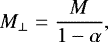 (22)
(22)
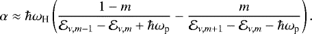
Velocity effects on the energy spectrum become of significant importance for large enough fields, particularly in the regime β ≫ 1 where Eq. (23) is derived using a basis of states {N, ν, m}. At very low field intensities (β≲1), a perturbative method based on states {n, l, m} would be more appropriate; however, the current expression for α is well behaved in this regime (where its effects are significantly reduced), and so we use this approach over the whole range of β. The application of the perturbation method demands energy corrections lower than the spacing of adjacent unperturbed levels (e.g.,  in large β). Consequently, this gives an upper limit to the magnitude of the transverse pseudo-momentum (Pavlov & Meszaros 1993)
 (24)
(24)
States for which the approximation given by Eq. (21) is valid are often called centered states (even when they could be weakly decentered states) because the electron wavefunction remains on average centered around the Coulomb well. In present work, anisotropy mass (M⊥) has been calculated with Eqs. (22) and (23) using energy data of Schimeczek & Wunner (2014). Some fits are given in Appendix A.6.
Solutions to Eq. (8) are usually found in the approximation of infinite nuclear mass (μ → me, γ → 1), here denoted  . The eigenvalues
  for finite mass may be then evaluated from the scaling relations (Pavlov-Verevkin & Zhilinskii 1980)
![\begin{equation*}\mathcal{E}=\frac{\mu}{m_{\text{e}}}\mathcal{E}_{\infty}\left[\left(\frac{m_{\text{e}}}{\mu}\right)^2\beta\right]-\left(\frac{m_{\text{e}}}{\mu}\right)^2 \hbar \omega_{\text{p}}(m+m_{\textrm{s}}), \end{equation*}](/articles/aa/full_html/2020/03/aa37413-19/aa37413-19-eq39.png) (25)
(25)
with ms = ± 1∕2 the spin quantum number of the electron. We note that Eq. (25) includes a scaling relation for the field intensity where  is evaluated. For the present case (electron and proton pairs) μ ≈ me and only the second term on the right-hand side of Eq. (25) is truly significant in occupation number calculations.
In the present work we adopt the energies  calculated by Schimeczek & Wunner (2014) which comprise spin-down levels (ms = −1∕2) emerging from zero-field states with principal quantum numbers n ≤ 15 and magnetic quantum numbers − 4 ≤ m ≤ 0. The energy values of states with ms = +1∕2 and m > 0 are respectively obtained by adding 4β and 4mβ to values
  measured in Rydberg units. Results from Schimeczek & Wunner (2014) let us find the scaling relations for the energy dependence on m and ν and the approximate energy curves for arbitrary bound states (see Appendix A). For instance, Figs. 1 and 2 show
  curves at ν = 0 and ν = 1 coming from the first twenty Bohr levels. These fits are valid for any B with relative errors lower than 1% and converge to the right limits at zero-field and very strong fields. Typical well-known energy expressions for strong fields (Eqs. (14)–(15)) show strong departures at β≲50 for the ground state and at much larger β for excited states. In particular, they cannot be used in the regime of magnetic white dwarfs (− 6.6≲logβ≲ − 0.6).
The accuracy of our energy fits varies for different levels and different field strengths. The mean relative error (σE) for the ground state does not exceed 0.4% in the range − 4 ≤ logβ ≤ 3 and falls below 0.1% in the MWD region. Other tightly bound states (ν = 0, − 4≤ m ≤−1) have relative errors of a few tenths of a percent in the MWD domain. General expression for ν ≥ 4 provides energies with σE typically between 2 and 4%, except peaks (≈7%) in a few hydrogen-like states (e.g., ν = 4, 8, 12).
A partial energy spectrum of the atom at rest taking into account finite nuclear mass is appreciated in Fig. 3. This shows the dependence with the field intensity of the states arising from the first four Bohr levels, and a comparison of our results from analytical expressions with Schimeczek & Wunner (2014) evaluations for spin-down states. The ionization energy of the atom, represented by the negative value of the solid curve labeled (ν, m) = (0, 0), increases monotonically with the field strength. As a consequence of the positive energy coupling with the field, spin-up states and those with positive magnetic quantum number increase their energies and move toward the continuum at relatively low field intensities, 0.01< β < 1. A second state migration toward the continuum occurs at high fields (β > 10, for the states showed in Fig. 3), due to finite nuclear-mass corrections affecting states with m < 0 (second term on the right-hand side of Eq. (25)). Only states with m = 0 remain bound for any field strength.
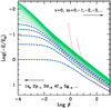 |
Fig. 1 Energies of tightly bound states (ν = 0) of atoms at rest and infinite nuclear mass, as a function of the magnetic field. Shown are the numerical results from Schimeczek & Wunner (2014) for the lowest five states (0 ≥ m ≥−5) with spin-down (dashed lines); our fits and extrapolations up to m = − 19 (solid lines); and the asymptotic approximations given by Eq. (14) for m = 0, −1 (dotted lines). |
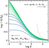 |
Fig. 2 As in Fig. 1, but for hydrogen-like states at ν = 1. The dotted line corresponds to predictions of Eq. (15) for m = 0. |
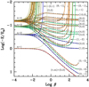 |
Fig. 3 Energies of magnetized atoms at rest coming from Bohr levels n = 1, 2, 3, and 4, as a function of the field intensity. Finite nuclear mass effects are included. Lines representfits used in this work for spin-down (solid) and spin-up (dotted) states. Symbols correspond to spin-down values calculated by Schimeczek & Wunner (2014). Some (ν, m) states are indicated on the plot. |
4.2 Decentered states
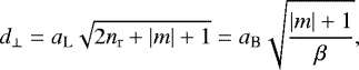
At very high pseudo-momentum of the atom motion across the field, the electron probability density is markedly shifted apart from the Coulomb center and approaches to the so-called relative guiding center (separation between the electron and proton guiding centers)
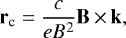 (26)
(26)

(rc = k⊥∕2β in atomic units). In this case, the atomic state becomes decentered and the dependence of the energy levels on k⊥ cannot be interpreted in terms of a mass anisotropy.
The transition between weakly to strongly decentered states have been studied in the regime of strong magnetic fields β ≳ 1 (Vincke et al. 1992; Potekhin 1994), where some useful analytical expressions have been given (Potekhin 1998; Potekhin et al. 2014). These expressions are adopted in the present work with minor changes to be extrapolated to low field intensity (for which we demand the condition  at k → 0). With energies measured in Rydberg units and rc in Bohr radii, the energy of decentered states is approximated by
 (28)
(28)
![\begin{equation*}\chi_0= \left\{ \begin{array}{@{}ll}\displaystyle 0, & \quad (\nu=0),\\ [2ex]\displaystyle \frac{2}{\mathcal{E}_{\infty}}, & \quad (\text{otherwise}),\\ \end{array} \right. \end{equation*}](/articles/aa/full_html/2020/03/aa37413-19/aa37413-19-eq48.png)
![\begin{equation*}\chi_1= \left\{ \begin{array}{@{}ll}\displaystyle \frac{r_{\textrm{c}}}{5-3m}+\frac{4}{\mathcal{E}_{\infty}^2}, & \quad (\nu\,{=}\,0),\\ [3ex]\displaystyle \left[\nu^2+2^{0.5\nu \log(1+\beta/150)}\right]r_c, & \quad (\text{even}~\nu>0),\\ [2ex]\displaystyle \left(\nu^2-1\right)r_c, & \quad (\text{odd}~\nu).\\ \end{array} \right. \end{equation*}](/articles/aa/full_html/2020/03/aa37413-19/aa37413-19-eq49.png)
Equations (28)–(30) contain the expected asymptotic value of the energy for large transverse pseudo-momentum,
 (31)
(31)
where the first term on the right-hand side is a CM correction to the total energy, and the second term represents the Coulomb energy (− e2∕rc) with the electron located on the magnetic well (i.e., to distance rc from the proton). On the other hand, Eq. (28) converges to the expected result corresponding to low transverse motions
 (32)
(32)
In practice, following Potekhin et al. (2014), the transition region  between centered and decentered states is identified by the intersection of curves given by Eqs. (21) and (28).
Figure 4 shows with solid lines the energies of some (ν, m) states (the most tightly bound ones and a few others) as a function of the transverse pseudo-momentum and for a strong field (β = 500). For low transverse motions, values grow quadratically with k⊥ according to the perturbative method (Eq. (21)). Because effective masses M⊥ are higher than M, the curves remain below the values obtained when the CM effects are ignored (dotted lines). At k⊥ larger than some critical value  (≈ 163, 111 and 80 au for the lowest states with ν = 0 and m = 0, − 1, − 2, respectively), states become decentered and the energies grow more slowly, according to Eq. (28). The asymptotic value reached by each state at high transverse motions depends exclusively on m. States with m < 0 rise above the ionization threshold at sufficiently high tranverse motions. In particular, the state (2, −1) is completely embedded in the continuous spectrum on the whole k⊥ domain due to CM effects. In the right extreme of the figure, the curves converge to the approximation given by Eq. (31) (dot-dashed lines), where the electron is expected to be located around the magnetic well to a distance rc from the proton.
It was suggested that general properties about the formation of decentered states remain valid at all field intensities (Vincke et al. 1992; Baye et al. 1992). Figure 5 explores the results on the low magnetic field domain, with the application of the present calculations to the case β = 0.1. Two main observations of Vincke et al. (1992) about the extrapolated properties of decentered states at low fields can been seen in this figure. First, centered states show low sensitivity to the coupling between internal and global motions. In this branch of the spectrum, the energy values (solid lines) are very similar to standard calculations without CM corrections (dotted lines) because M⊥ ≈ M. Second, decentered states become weakly bound, and quickly converge to a unique curve coincident with the approximation Eq. (31); i.e., when k⊥ exceeds a critical value, states become abruptly decentered with the electron around the magnetic well.
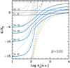 |
Fig. 4 Particle movement effects on bound state energies. Solid lines represent energies (without kinetic contribution from motion along the field) of magnetized atoms for a few states (ν, m) as a functionof the transverse pseudo-momentum, at β = 500 (B = 2.35 × 10¹² G). Results without finite-velocity effects are indicated by dotted lines. Approximations based on Eqs. (21), (28), and (31) are displayed as short-dashed, long-dashed [only for (0, 0), (1, 0) and (2, −1) states], and dot-dashed lines, respectively. |
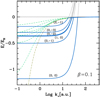 |
Fig. 5 As in Fig. 4, but for β = 0.1 (B = 4.70 × 10⁸ G). Long-dashed lines are not shown since they coincide with the dotted lines. |
5 Ionization equilibrium
The condition for the ionization equilibrium of a gas of magnetized atomic hydrogen (H ↔H+ + e−) can be written in the usual form based on the chemical potentials μi of the involved species,
 (33)
(33)
The chemical potential expressions adopted in the present work for electrons, protons, and atoms are given below.
Electrons: the energy of a free electron in the field is composed by the Landau levels (including spin-field coupling with giromagnetic ratio ge = 2) plus the kinetic contribution from the motion parallel to the field,
 (34)
(34)
The spin degeneracy is one (σz = −1) for the ground Landau level, and two (σz = ±1) for excited levels. These energies have a multiplicity of one in j = 0 and two otherwise. From Fermi statistics it follows that the electron density in the gas is (Potekhin et al. 1999)
![\begin{equation*}n_{\text{e}} = \frac{\hbar\omega_{\text{e}}}{\sqrt{\pi}{k_{\textrm{B}}} T\lambda_{\text{e}}^3} \left[I_{-1/2}\left(\frac{\mu_{\text{e}}}{{k_{\textrm{B}}} T}\right) +2\sum_{j=1}^{\infty} I_{-1/2}\left(\frac{\mu_{\text{e}}}{{k_{\textrm{B}}} T}-\frac{\hbar\omega_{\text{e}} j}{{k_{\textrm{B}}} T}\right) \right], \end{equation*}](/articles/aa/full_html/2020/03/aa37413-19/aa37413-19-eq56.png) (35)
(35)
with kB the Boltzmann constant, T the gas temperature, μe the electron chemical potential,  the electron thermal wavelength, and Is(x) the Fermi integral of order s. In the classical limit (low density or high temperature, so that − βμe ≫ 1,
  ), Eq. (35) reduces to the form given by Gnedin et al. (1974). In this case the electron chemical potential is given by
![\begin{equation*}\frac{\mu_{\text{e}}}{{k_{\textrm{B}}} T} = \ln\left(\frac{n_{\text{e}}\lambda_{\text{e}}^3}{2}\right) +\ln\left[\left(\frac{2{k_{\textrm{B}}} T}{\hbar\omega_{\text{e}}}\right)\tanh\left(\frac{\hbar\omega_{\text{e}}}{2{k_{\textrm{B}}} T}\right)\right]. \end{equation*}](/articles/aa/full_html/2020/03/aa37413-19/aa37413-19-eq59.png) (36)
(36)
The last term on the right-hand side of Eq. (36) represents the chemical potential excess (with respect to the ideal gas contribution) due to the electron interaction with the magnetic field,
![\begin{equation*}\frac{\mu^{\text{ex}}_{\text{e}}}{{k_{\textrm{B}}} T} =\ln\left[\frac{\tan{\textrm{h}}\left(\eta\right)}{\eta}\right],\hskip.3in \end{equation*}](/articles/aa/full_html/2020/03/aa37413-19/aa37413-19-eq60.png) (37)
(37)
which depends on the parameter defined by
 (38)
(38)
The asymptotic behaviors of  are
are
![\begin{equation*} \frac{\mu^{\text{ex}}_{\text{e}}}{{k_{\textrm{B}}} T} = \left\{ \begin{array}{@{}ll}\displaystyle -\eta^2/3+ O(\eta^4), & \quad (\eta\ll1),\\ [1ex]\displaystyle -\ln(\eta), & \quad (\eta\,{\gg}\,1).\\ \end{array} \right. \end{equation*}](/articles/aa/full_html/2020/03/aa37413-19/aa37413-19-eq63.png) (39)
(39)
Protons: the energy of a proton in the field is given by
 (40)
(40)
with ωp = (me∕mp)ωe. The zero-point and spin-field interaction energies of protons are omitted in Eq. (40) because they do not affect the chemical equilibrium. Classical statistics yields
![\begin{equation*}\frac{\mu_{\text{p}}}{{k_{\textrm{B}}} T} = \ln\left(n_{\text{p}}\lambda_{\text{p}}^3\right) +\ln\left[\frac{1-\exp\left(-\hbar\omega_{\text{p}}/{k_{\textrm{B}}} T\right)} {\hbar\omega_{\text{p}}/{k_{\textrm{B}}} T}\right], \end{equation*}](/articles/aa/full_html/2020/03/aa37413-19/aa37413-19-eq65.png) (41)
(41)
where  is the proton thermal wavelength, and np the number density of protons. The chemical potential excess of protons is given by
![\begin{equation*}\frac{\mu^{\text{ex}}_{\text{p}}}{{k_{\textrm{B}}} T} = \ln\left[\frac{1-e^{-q\eta}}{q\eta}\right], \end{equation*}](/articles/aa/full_html/2020/03/aa37413-19/aa37413-19-eq67.png) (42)
(42)
with q ≡ 2me∕mp ≈ 0.00108923, and the limits
![\begin{equation*}\frac{\mu^{\text{ex}}_{\text{p}}}{{k_{\textrm{B}}} T} = \left\{ \begin{array}{@{}ll}\displaystyle -q\eta/2+ O(\eta^2), & \quad (\eta\ll1),\\[3pt] \displaystyle 6.82228-\ln(\eta), & \quad (\eta\,{\gg}\,1).\\ \end{array} \right. \end{equation*}](/articles/aa/full_html/2020/03/aa37413-19/aa37413-19-eq68.png) (43)
(43)
Atoms: the energy spectrum of bound states of atoms have been detailed in previous section. Energies of centered and decentered states may be written in the general form
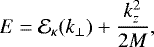 (44)
(44)
where κ is the set of quantum numbers of a bound state, i.e., κ = {n, l, m, ms} at low field and κ = {N, ν, m, ms} at strong field, both connected by the relationships (16)–(19). In addition, the quantity  in (44) is straightforwardly derived from either Eq. (21) or (28), taking their minimum value.
The chemical potential of magnetized atoms may be written in the usual form,
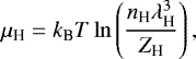 (45)
(45)
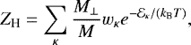
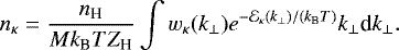
with 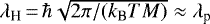 , nH the number density of atoms, and ZH a partition function which contains non-ideal effects and the coupling of internal and transverse kinetic energies,
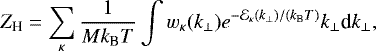 (46)
(46)
wκ (k⊥) being the so-called occupational probability of the state (κ, k⊥). Equations (45) and (46) are derived in the framework of the Helmholtz free-energy method (Potekhin et al. 1999). This method is valid at a moderately low-density regime, usually ρ < 10−2 g cm−3 in field-free conditions (Hummer & Mihalas 1988; Saumon & Chabrier 1991), although the well-known reduction of effective sizes of atoms due to the magnetic field may push this limit to a higher value. At low temperatures, when most atoms have  , the partition function reduces to (Pavlov & Meszaros 1993)
 (47)
(47)
where now  is the energy of the rest atom. Clearly, ZH converges to a standard internal partition function when the magnetic field is switch off (M⊥→ M).
A precise account of particle interactions in the evaluation of species populations at equilibrium, demands the use of quantum-mechanics calculations of collective energies for a reference atom and its nearest neighbor particles, all them under the action of a magnetic field. To the best knowledge of the authors, these calculations are not available. Since a study of particle interaction effects on the chemical equilibrium is beyond the scope of the present paper, we adopt here a simple scheme (Hummer & Mihalas 1988; Lai 2001), which is typically used in model atmospheres of white dwarf stars (e.g., Bergeron et al. 1991; Rohrmann et al. 2002)1. In this formalism, the occupation probability is given by a product of two contributions
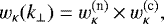 (48)
(48)
which express a reduction of the phase space available for the state κ as a consequence of statistically independent perturbations of the atom due to neutral ( ) and charged (
 ) particles. The neutral contribution is written as
![\begin{equation*}w^{(\text{n})}_{\kappa}(k_{\perp}) = \exp\left[-n_{\text{H}} v_{\kappa}(k_{\perp})\right], \end{equation*}](/articles/aa/full_html/2020/03/aa37413-19/aa37413-19-eq80.png) (49)
(49)
where vκ(k⊥) is the effective volume of the atom in the state (κ, k⊥), and it is assumed that bound particles different to atoms (molecules, particle chains, negative ions) are not present in the gas. Equation (49) results from changes in the gas entropy due to a reduction of the available volume for the atom due to overlapping of electron configurations in the system. On the other hand, for the evaluation of  we use the results of Nayfonov et al. (1999). This term can be interpreted as a lowering of the continuum energy level yielded by electric microfield fluctuations originated from neighboring charged particles.
High excited states usually have large atomic size and are very weakly bound, so that Eq. (48) gives a low occupation prob- ability for them. Moreover, wκ assures the convergence of the partition function in two ways, yielding a finite number of bound states effectively occupied and an upper value for the allowed values of the pseudo-momentum. Because the limit of atomic sizes (d) allowed in a gas with mass density ρ (roughly πd3∕6 = M∕ρ), there is a maximum value of pseudo-momentum for decentered states (d ≳ rc)
![\begin{equation*}k_{\perp}^{\text{top}}\la \frac{2\beta}{a_{\text{B}}}\left(\frac{6M}{\pi\rho}\right)^{1/3} \approx 5.568 \frac{\beta}{\rho[\text{c.g.s.}]^{1/3}}\;\text{au} \end{equation*}](/articles/aa/full_html/2020/03/aa37413-19/aa37413-19-eq82.png) (50)
(50)
Accordingly, integration on Eq. (46) is performed with Gaussian quadrature in the range 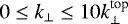 to ensure an appropriate evaluation of ZH.
5.1 Effective atomic sizes
The electron cloud (mean probability distribution) in a non-moving atom changes from spherical symmetry at β ≪ 1 to cylindrical at β ≫ 1. In the zero-field limit, the effective radius of a state κ = (n, l, m) is
![\begin{equation*}r_{nl}\,{=}\,\frac{a_{\text{B}}}{2}\left[3n^2-l(l+1)\right], \end{equation*}](/articles/aa/full_html/2020/03/aa37413-19/aa37413-19-eq84.png) (51)
(51)
with aB the Bohr radius. On the other hand, at very intense fields the root mean square of the transversal radius of states κ = (N, ν, m) tends to the Landau state value,
 (52)
(52)
where  is the Larmor radius and the last expression in Eq. (52) corresponds to bound states (nr = 0).
An analysis of the spatial probability distribution of the electron for a number of eigenenergy states using data from Ruder et al. (1994) and Schimeczek & Wunner (2014), let us find approximated fits for the longitudinal size and transverse radius of the wavefunctions
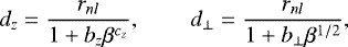 (53)
(53)
with bz, b⊥, and cz numerical parameters depending on the state κ. Some valuesare given in Table 2. The effective volume of an atom at rest or moving is approximated by
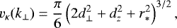 (54)
(54)
where r* = r*(k⊥) measures the mean electron-proton separation, which is the distance between the mean positions of proton and electron in an atom with transverse pseudo-momentum k⊥. In particular, r* ≈ 0 for centered states and r*→ rc (Eq. (27)) for strongly decentered states. Analytical expressions can be used to represent r* following a smooth transition between these limits. However, for numerical calculations in relatively low densities (ρ < 0.01 g cm−3) or moderate low field intensities (β≲1), it is possible to adopt
![\begin{equation*}r_* = \left\{ \begin{array}{@{}ll}\displaystyle 0, & \quad (\text{centered state}),\\ [1ex]\displaystyle r_{\text{c}}, & \quad (\text{decentered state}),\\ \end{array} \right. \end{equation*}](/articles/aa/full_html/2020/03/aa37413-19/aa37413-19-eq89.png) (55)
(55)
At the mentioned conditions, we have verified that the occupation probability of decentered states deviates from unity mostly when approximation Eq. (31) is valid.
5.2 Law of mass action
According to condition (33) and Eqs. (36), (41), and (45), the equilibrium constant  for the ionization process of hydrogen in a magnetic field is given by
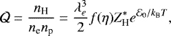 (56)
(56)
 (> 0) is the ionization energy of magnetized atoms, and the factor f(η) comes from the chemical potential excess of electron and proton,
 (58)
(58)
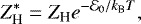
 represents the partition function defined with the zero-point energy in the ground state (
 ), and therefore is a measure of atomic excitation degree. At low or moderate fields and sufficiently low temperature (far away of pressure ionization conditions),
  takes a minimum value between one and two depending of the occupation fraction of the spin-up state at (ν, m) = (0, 0).
Finally, the number density of a state κ reads
 (59)
(59)
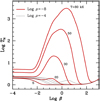 |
Fig. 6 Values of the partition function |

6 Results
In this section, we show the calculations of the equilibrium ionization of magnetized hydrogen carried out for temperatures and densities present in MWD atmospheres. MWDs constitute about 10% of the total population of single white dwarfs. As their non-magnetic analogs, they have thin non-degenerate atmospheres and are mostly composed of hydrogen. Several hundred MWDs are currently known (Kepler et al. 2014). They have effective temperatures Teff ≈ 5000–80 000 K and gravity surfaces around logg ≈ 8, where the gas density in their atmospheres roughly ranges from 10−12 to 10−3 g cm−3.
In Fig. 6 the run of the partition function versus the magnetic field intensity is shown for several temperatures and densities. Curves at T = 5000 K correspond to conditions where the electronic excitations are neglegible in the zero-field limit. For this temperature, the partition function decreases to unity at logβ≲ − 1.5 (B≲108 G) as the energy of the spin-up state in the level n = 1 shifts toward the continuum. At larger fields,  slowly increases due to contributions of tightly bound states (ν = 0, m = −1, − 2, …) coming from high energies (see Fig. 3). Electronic excitations take place for higher temperatures. In particular, isotherms with T ≥30 000 K and ρ = 10−8 g cm−3 (solid lines in the figure) show a strong increase in
  at intermediate field values due to contributions from decentered states. As the field rises, the partition function curves finally drop to mini- mum values (similar to the low temperature results) because large energy differences between decentered states and the tightly bound state (v, m) = (0, 0), which grow gradually with β. Furthermore, the partition function takes lower values at high densities, as can be seen for ρ = 10−4 g cm−3 (dotted lines in Fig. 6). This is caused by decreased occupation probabilities of excited states, especially decentered states, which are destroyed due to their large atomic sizes.
Figure 7 shows the neutral atom fraction, xH = nH∕(nH + np), derived from the equilibrium condition (56) and the barionic conservation equation assumed in the present work (ρ∕M = nH + np). Magnetic effects on the equilibrium constant coming from free electrons and protons are represented by the factor f(η), which decreases monotonically from one to zero as the field intensity grows. Therefore, f(η) favors the gas ionization. However its effect is usually countered by other contributions to  , particularly by
  at moderate fields and by the Boltzmann factor (containing the ionization energy
  ) at intense fields. In fact, as the field strength is raised over β ≈ 0.01, the Boltzmann factor strongly increases (through the ionization energy) and ultimately overcomes the equilibrium constant. As a consequence, the gas tends to a full recombination at high magnetic fields. The abundance of atoms grows as the density increases to ρ ≈ 10−4 g cm−3 (dotted lines in Fig. 7), while the ground state and other tightly bound states remain unperturbed (occupation probability close to unity).
Various effects of the magnetic field on the gas in the conditions of atmospheres of MWDs may be explored. On the one hand, Fig. 8 illustrates on a plane of temperature versus magnetic strength (in logarithmic scales) the mean values determined for a sample of MWDs (Külebi et al. 2009), representing physical conditions in their atmospheres. The lines show percentages of the spin-down state contribution in the partition function. It can be clearly seen in the figure that spin-up states are removed of the partition function for log β > −3 just over the bulk of strong MWDs. This result is largely independent of the density in the regime studied.
On the other hand, Fig. 9 shows the importance of decentered states relative to centered ones on the partition function  . Decentered states become dominant at high temperatures and intermediate values of the magnetic field, with peaks around β ≈ 0.1, just where the strongest MWDs are located. The contribution of decentered states extends to lower temperatures and a wide range of field values for low densities (ρ = 10−12 g cm−3 in the figure). According to these results, decentered states could be present in the outer layers of hot MWDs (Teff ≳ 20 000 K) with megagauss fields and in deep atmospheric layers of the strongest magnetic objects. Present calculations are based on extrapolations toward low magnetic fields of results of CM effects derived at higher fields, following the expected values by Vincke et al. (1992) and Baye et al. (1992). It is clear that valuable insight can be gained if new accurate studies are aimed to analyze the couplingbetween the internal energy of atoms and their transverse movements at moderate and weak magnetic fields. These studies will be useful to search and identify possible spectroscopic signatures of decentered states in the spectrum of MWDs.
Figure 10 displays the predicted curves of the iso-abundance of atoms in the usual diagram of temperatureagainst field intensity. It is immediately clear that the abundance of neutral atoms does not stay constant along the sample of known MWDs. The onset of magnetic recombination occurs approximately at log β = −2 (B ≈ 5 × 10⁷ G), decreasing the gas ionization for the strongest MWDs observed. The electronic recombination increases with the gas density in the whole density regime of these atmospheres, since the lowest energy states remain barely perturbed by particle neighbors at ρ≲10−3 g cm−3. It is worth noting that changes in the ionization equilibrium can affect the structure of an atmosphere, specially through its influence on the radiative opacities.
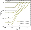 |
Fig. 7 Concentration of atoms along isotherms for two densities. Temperatures are indicated on the plot for the case ρ = 10−8 g cm−3. The same T values correspond to ρ = 10−4 g cm−3, decreasing from bottom to top. |
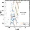 |
Fig. 8 Contributions (in percent) of spin-down states to the partition function |

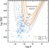 |
Fig. 9 Same as Fig. 8, but for the fraction (in percent) of partition function |

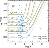 |
Fig. 10 Same as Fig. 8, but for concentrations of neutral atoms in the gas. Values of xH are indicated on the plot for ρ = 10−8 g cm−3. |
7 Final remarks
We presented a general method for calculating the partition function of hydrogen atoms in a wide range of field strengths. The evaluations rely on fits of accurate energy evaluations of atoms at rest, complemented by CM effects on internal atomic structure, particularly those that arise from thermal motions across the magnetic field. The work benefited from mathematical relations that express the correspondence between sets of quantum numbers at the limits of zero-field and very strong fields. These relations are given here for the first time.
To our knowledge, this is also the first time that a detailed treatment of the atomic hydrogen abundance under ionization process has been undertaken for magnetic fields from zero to very high strengths. In particular, we extended the analysis of ionization balance of hydrogen to include the regime of moderate magnetic fields (β≲1, B≲109 G). This compresses the realm of magnetic white dwarfs, where the effects of the field on the chemical equilibrium are not included in current atmosphere models. We found, however, that these effects cannot be ignored at least for the strongest MWDs. Although these fields are much lower than those achieved in neutron stars, they are sufficiently strong to modify the ionization equilibrium. Future work will be devoted to the formation of molecules and other species (which are also altered by the magnetic field) in order to obtain reliable occupation numbers of atomic states and free particles.
It was shown here that decentered states could be present in the surface of strong MWDs, being the dominant contribution of the partition function in some cases (hot and strongly magnetic atmospheres). If this phenomenon occurs, it can have effects on the energy distribution emitted by these stars. A definitive analysis of the decentered state’s role on MWDs requires further investigation on the formation of these states at weak magnetic fields and, in general, on the relationship between the movement of atoms across the field and their internal energy spectrum.
Acknowledgements
We wish to thank C. Schimeczek, who kindly sent us his energy evaluations for magnetized atoms at rest, and José Ignacio Castro for useful discussions. Authors thank the support of the MINCYT (Argentina) through Grant No. PICT 2016-1128.
Appendix A Analytical fits
We show analytic fits to the energy data of Schimeczek & Wunner (2014) for bound states of hydrogen atoms at rest in the approximation of infinite nuclear mass. Results are expressed in logarithmic scales. In this appendix we adopt the notation (log ≡ log10)
 (A.1)
(A.1)
 (A.2)
(A.2)
 (A.3)
(A.3)
![\begin{equation*} \epsilon_{\nu}=-2\log\left[\text{Int}\left(\frac{\nu+1}2\right)\right]. \end{equation*}](/articles/aa/full_html/2020/03/aa37413-19/aa37413-19-eq108.png) (A.4)
(A.4)
Fits were performed in the range − 4 ≤ logβ ≤ 3, although they are well behaved in the full non-relativistic domain (log β < 4)2. In particular, they converge to the right limits at β = 0 and logβ ≫ 1. Fitting equations are organized bythe quantum number ν.
A.1 States ν = 0
Energies of tighly bound states (ν = 0, m = 0, −1, −2, …) are represented by
![\begin{equation*}\epsilon = \left\{ \begin{array}{@{}ll}\displaystyle 1+\frac{\epsilon_n-1}{1+a_1 \exp\{a_2[x-x_a-0.1(x-x_a)^2]\}}, & (x<x_a)\\ [3ex]\displaystyle \epsilon_a + (\epsilon_b-\epsilon_a)\left(\frac{x-x_a}{x_b-x_a}\right)^{1.22}, & (x_a<x<x_b)\\ [3ex]\displaystyle \epsilon_b +(\epsilon_c-\epsilon_b)\left(\frac{x-x_b}{3-x_b}\right)^{0.92}, & (x_b<x)\\ \end{array} \right. \end{equation*}](/articles/aa/full_html/2020/03/aa37413-19/aa37413-19-eq109.png) (A.5)
(A.5)
The m-dependence of parameters (xa, xb, ϵa, ϵb, ϵc,  ) is very well adjusted by
![\begin{equation*}f=b_0+b_1 [\log(1+|m|)]^{b_2}. \end{equation*}](/articles/aa/full_html/2020/03/aa37413-19/aa37413-19-eq113.png) (A.8)
(A.8)
The values of coefficients bj are listed in Table A.1. Equation (A.5) fits the results of Schimeczek & Wunner (2014) with relative error within a few percentage points (see Fig. 1).
A.2 States ν = 1
Energies of states with ν = 1 are given bya global approximation
![\begin{equation*}\epsilon= \epsilon_{\nu} + \frac{\epsilon_n - \epsilon_{\nu}} {1+a_1\exp\{a_2(x-x_b)[1-\delta(x-x_b)]\}}, \end{equation*}](/articles/aa/full_html/2020/03/aa37413-19/aa37413-19-eq114.png) (A.9)
(A.9)
 (A.10)
 (A.11)
with n = |m| + 2, δ = 0.26 except at |m| = 1, 2, 3 (where δ = 0.20, 0.22, 0.24, respectively) and x > xb (δ = 0). Quantities xb, ϵb, and  are calculated with help of Eq. (A.8) and Table A.1. The performance of fits at ν = 1 is shown in Fig. 2.
A.3 States ν = 2
Energies of states corresponding to ν = 2 are represented by a piecewise approximation. For x ≤ xb, we use Eq. (A.9) with n = |m| + 2, δ = 0.2, supplemented by Eq. (A.8) with the data in Table A.1. For x > xb, ϵ is given by
![\begin{equation*} \epsilon= \epsilon_b + \frac{2}{\pi}(\epsilon_b-\epsilon_{n=1}) \tan^{-1}\left[\frac{\pi\epsilon'_b(x-x_b)}{2(\epsilon_b-\epsilon_{n=1})} [1+\xi(x-x_b)], \right], \end{equation*}](/articles/aa/full_html/2020/03/aa37413-19/aa37413-19-eq118.png) (A.12)
(A.12)
![\begin{equation*} \xi = -0.0125 +0.030456[\log(1+m_*)]^{1.134} \end{equation*}](/articles/aa/full_html/2020/03/aa37413-19/aa37413-19-eq119.png)
and m* = min(|m|, 4).
A.4 States ν = 3
We adopt a piecewise approximation for energies at ν = 3. As before, Eq. (A.9) is applied for x ≤ xb, with n = |m| + 3 and δ = 0, 0.08, 0.13, 0.15, 0.165, and 0.17 for |m| = 0, 1, 2, 3, 4, 5, and ≥ 6, respectively. Parameters are represented by Eq. (A.8) with the data in Table A.1. For x > xb, the following expression is used:
![\begin{equation*} \epsilon= \epsilon_b + \frac{(\epsilon_{\nu}-\epsilon_b)(x-x_b)} { \{[(\epsilon_{\nu}-\epsilon_b)/\epsilon'_b]^q+(x-x_b)^q\}^{1/q} }, \end{equation*}](/articles/aa/full_html/2020/03/aa37413-19/aa37413-19-eq120.png) (A.14)
(A.14)
with q = 2.5.
A.5 States ν ≥4
The energy of state with ν ≥ 4 is calculatedas follows:
![\begin{equation*}\epsilon = \left\{ \begin{array}{@{}ll}\displaystyle \epsilon_a + \frac{(\epsilon_a-\epsilon_{n})(x-x_a)} {\left[c_a^2+(x-x_a)^2\right]^{1/2}}, & (x\le x_a)\\ [3ex]\displaystyle \epsilon_a + (\epsilon_*-\epsilon_a)\left[ \frac{(\epsilon_b-\epsilon_*) \zeta + (\epsilon_b-\epsilon_a) (x-x_*)^2} {c_*+(\epsilon_b-\epsilon_a)^2 (x-x_*)^2} \right], & (x_a,x_b)\\ [3ex]\displaystyle \epsilon_b + \frac{(\epsilon_{\nu}-\epsilon_b)(x-x_b)} {\left[c_b^2+(x-x_b)^2\right]^{1/2}}, & (x_b\le x)\\ \end{array} \right. \end{equation*}](/articles/aa/full_html/2020/03/aa37413-19/aa37413-19-eq121.png) (A.15)
(A.15)


In addition, xa, xb, ϵa, ϵb, ya, yb are fitted by Eq. (A.8). In turn, parameters bj (j = 0, 1, 2) in this equation are calculated as follows:
![\begin{equation*}b_0[x_a] = \left\{ \begin{array}{@{}ll}\displaystyle -1.1 \tau -1.154902 -2.087178 \Delta^{1.082710}, & (\text{even}~\nu)\\ [1ex]\displaystyle -\tau -1.18 -2.312886\Delta^{0.7737455}, & (\text{odd}~\nu)\\ \end{array} \right. \end{equation*}](/articles/aa/full_html/2020/03/aa37413-19/aa37413-19-eq124.png) (A.18)
(A.18)
![\begin{equation*} b_0[x_b] = \left\{ \begin{array}{@{}ll}\displaystyle -0.522879, & (\text{even}~\nu)\\ [1ex]\displaystyle -1.154902, & (\text{odd}~\nu)\\ \end{array} \right. \end{equation*}](/articles/aa/full_html/2020/03/aa37413-19/aa37413-19-eq125.png) (A.19)
(A.19)
![\begin{equation*} b_0[\epsilon_a] = \left\{ \begin{array}{@{}ll}\displaystyle -0.68 -1.176143\Delta^{0.8685913}, & (\text{even}~\nu)\\ [1ex]\displaystyle -0.9558838 -1.069160\Delta^{0.8065575}, & (\text{odd}~\nu)\\ \end{array} \right. \end{equation*}](/articles/aa/full_html/2020/03/aa37413-19/aa37413-19-eq126.png) (A.20)
(A.20)
![\begin{equation*} b_0[\epsilon_b] = \left\{ \begin{array}{@{}ll}\displaystyle -0.8867395 -1.744739\Delta^{1.095173}, & (\text{even}~\nu)\\ [1ex]\displaystyle -1.12 -1.707775\Delta^{1.119483}, & (\text{odd}~\nu)\\ \end{array} \right. \end{equation*}](/articles/aa/full_html/2020/03/aa37413-19/aa37413-19-eq127.png) (A.21)
(A.21)
![\begin{equation*} b_0[y_a] = \left\{ \begin{array}{@{}ll}\displaystyle 0.02 -0.034\tau +\frac{0.2}{\nu^{1.1} + 3}, & (\text{even}~\nu)\\ [2ex]\displaystyle 0.013-0.034\tau +\frac{0.2}{\nu^{0.74} +6}, & (\text{odd}~\nu)\\ \end{array} \right. \end{equation*}](/articles/aa/full_html/2020/03/aa37413-19/aa37413-19-eq128.png) (A.22)
(A.22)
![\begin{equation*} b_0[y_b] = \left\{ \begin{array}{@{}ll}\displaystyle 0.3780437\nu^{-0.9572978}, & (\text{even}~\nu)\\ [2ex]\displaystyle 0.3480917\nu^{-0.9508739}, & (\text{odd}~\nu)\\ \end{array} \right. \end{equation*}](/articles/aa/full_html/2020/03/aa37413-19/aa37413-19-eq129.png) (A.23)
(A.23)
![\begin{equation*} b_1[x_a] = \left\{ \begin{array}{@{}ll}\displaystyle -0.01890508, & (\text{even}~\nu)\\ [1ex]\displaystyle 0.1044253, & (\text{odd}~\nu)\\ \end{array} \right. \end{equation*}](/articles/aa/full_html/2020/03/aa37413-19/aa37413-19-eq130.png) (A.24)
(A.24)
![\begin{equation*} b_1[x_b] = \left\{ \begin{array}{@{}ll}\displaystyle -0.95 -1.1\nu^{-0.4}, & (\text{even}~\nu)\\ [1ex]\displaystyle -0.1 -2\nu^{-0.4}, & (\text{odd}~\nu)\\ \end{array} \right. \end{equation*}](/articles/aa/full_html/2020/03/aa37413-19/aa37413-19-eq131.png) (A.25)
(A.25)
![\begin{equation*} b_1[\epsilon_a] = \left\{ \begin{array}{@{}ll}\displaystyle -0.2 -1.1\nu^{-0.4}, & (\text{even}~\nu)\\ [1ex]\displaystyle -0.2 -0.9\nu^{-0.4}, & (\text{odd}~\nu)\\ \end{array} \right. \end{equation*}](/articles/aa/full_html/2020/03/aa37413-19/aa37413-19-eq132.png) (A.26)
(A.26)
![\begin{equation*} b_1[\epsilon_b] = \left\{ \begin{array}{@{}ll}\displaystyle -2.487767\nu^{-0.9652760}, & (\text{even}~\nu)\\ [1ex]\displaystyle -2.713701\nu^{-1.000845}, & (\text{odd}~\nu)\\ \end{array} \right. \end{equation*}](/articles/aa/full_html/2020/03/aa37413-19/aa37413-19-eq133.png) (A.27)
(A.27)
![\begin{equation*} b_1[y_a] = \left\{ \begin{array}{@{}ll}\displaystyle 0.1438085, & (\text{even}~\nu)\\ [1ex]\displaystyle 0.1457385, & (\text{odd}~\nu)\\ \end{array} \right. \end{equation*}](/articles/aa/full_html/2020/03/aa37413-19/aa37413-19-eq134.png) (A.28)
(A.28)
![\begin{equation*} b_1[y_b] = \left\{ \begin{array}{@{}ll}\displaystyle 0.8265754\nu^{-0.9347425}, & (\text{even}~\nu)\\ [1ex]\displaystyle 1.0286911\nu^{-0.9818393}, & (\text{odd}~\nu)\\ \end{array} \right. \end{equation*}](/articles/aa/full_html/2020/03/aa37413-19/aa37413-19-eq135.png) (A.29)
(A.29)
![\begin{equation*} b_2[x_a] = \left\{ \begin{array}{@{}ll}\displaystyle 0.5904491, & (\text{even}~\nu)\\ [1ex]\displaystyle 0.7094884, & (\text{odd}~\nu)\\ \end{array} \right. \end{equation*}](/articles/aa/full_html/2020/03/aa37413-19/aa37413-19-eq136.png) (A.30)
(A.30)
![\begin{equation*} b_2[x_b] = \left\{ \begin{array}{@{}ll}\displaystyle 0.85 +1.1\nu^{-0.4}, & (\text{even}~\nu)\\ [1ex]\displaystyle 0.90 +1.5\nu^{-0.4}, & (\text{odd}~\nu)\\ \end{array} \right. \end{equation*}](/articles/aa/full_html/2020/03/aa37413-19/aa37413-19-eq137.png) (A.31)
(A.31)
![\begin{equation*} b_2[\epsilon_a] = \left\{ \begin{array}{@{}ll}\displaystyle 0.6 +0.8\Delta^{0.4}, & (\text{even}~\nu)\\ [1ex]\displaystyle 0.7 +0.73\Delta^{0.4}, & (\text{odd}~\nu)\\ \end{array} \right. \end{equation*}](/articles/aa/full_html/2020/03/aa37413-19/aa37413-19-eq138.png) (A.32)
(A.32)
![\begin{equation*} b_2[\epsilon_b] = \left\{ \begin{array}{@{}ll}\displaystyle 1.209001, & (\text{even}~\nu)\\ [1ex]\displaystyle 1.251972, & (\text{odd}~\nu)\\ \end{array} \right. \end{equation*}](/articles/aa/full_html/2020/03/aa37413-19/aa37413-19-eq139.png) (A.33)
(A.33)
![\begin{equation*} b_2[y_a] = \left\{ \begin{array}{@{}ll}\displaystyle 1.596943, & (\text{even}~\nu)\\ [1ex]\displaystyle 1.603306, & (\text{odd}~\nu)\\ \end{array} \right. \end{equation*}](/articles/aa/full_html/2020/03/aa37413-19/aa37413-19-eq140.png) (A.34)
(A.34)
![\begin{equation*} b_2[y_b] = \left\{ \begin{array}{@{}ll}\displaystyle 1.114659, & (\text{even}~\nu)\\ [1ex]\displaystyle 1.181565, & (\text{odd}~\nu)\\ \end{array} \right. \end{equation*}](/articles/aa/full_html/2020/03/aa37413-19/aa37413-19-eq141.png) (A.35)
(A.35)
![\begin{equation*}\Delta = \left\{ \begin{array}{@{}ll}\displaystyle \log(\nu)-\log(4), & (\text{even}~\nu)\\ [3ex]\displaystyle \log(\nu)-\log(5), & (\text{odd}~\nu)\\ \end{array} \right. \end{equation*}](/articles/aa/full_html/2020/03/aa37413-19/aa37413-19-eq142.png)
![\begin{equation*}\tau=t-\text{Int}[t] \end{equation*}](/articles/aa/full_html/2020/03/aa37413-19/aa37413-19-eq143.png)
![\begin{equation*}t = 2\sqrt{\left[\frac12\left(\nu+\frac12\right)\right]}\pm 2, \end{equation*}](/articles/aa/full_html/2020/03/aa37413-19/aa37413-19-eq144.png)
with sign + (−) for even (odd) ν.
In order to avoid crossing levels, when current expressions give xa > xb the corresponding mean values (xa + xb)∕2 and (ϵa + ϵb)∕2 are assigned for xa = xb and ϵa = ϵb, respectively.
A.6 Effective mass of transverse motions
The effective mass given by Eqs. (22) and (23) can be approximated by
 (A.39)
With energy values calculated by Schimeczek & Wunner (2014), we found for m = 0
![\begin{equation*} b= \left\{ \begin{array}{@{}ll}\displaystyle 1.78\,{\times}\,10^{-3}(1+\nu)^{2.58}, & \quad (\text{even}~\nu),\\ [1ex]\displaystyle 10^{-3}(2+\nu)^{3}, & \quad (\text{odd}~\nu).\\ \end{array} \right. \end{equation*}](/articles/aa/full_html/2020/03/aa37413-19/aa37413-19-eq146.png) (A.40)
(A.40)
![\begin{equation*} c= \left\{ \begin{array}{@{}ll}\displaystyle 1+0.27\log(\nu+0.4), & \quad (\text{even}~\nu),\\ [1ex]\displaystyle 1.02+0.3\log(\nu+0.4), & \quad (\text{odd}~\nu).\\ \end{array} \right. \end{equation*}](/articles/aa/full_html/2020/03/aa37413-19/aa37413-19-eq147.png) (A.41)
(A.41)
References
- Avron, J. E., Herbst, I. W., & Simon, B. 1978, Ann. Phys., 114, 431 [NASA ADS] [CrossRef] [Google Scholar]
- Aznar Cuadrado, R., Jordan, S., Napiwotzki, R., et al. 2004, A&A 423, 1081 [NASA ADS] [CrossRef] [EDP Sciences] [Google Scholar]
- Bartnik, A. C., Efros, A. L., Koh, W.-K., Murray, C. B., & Wise, F. W. 2010, Phys. Rev. B, 82, 195313 [NASA ADS] [CrossRef] [Google Scholar]
- Baye, D., Clerbaux, N., & Vincke, M. 1992, Phys. Lett. A, 166, 135 [NASA ADS] [CrossRef] [Google Scholar]
- Bergeron, P., Wesemael, F., & Fontaine, G. 1991, ApJ, 367, 253 [NASA ADS] [CrossRef] [Google Scholar]
- Burkova, L. A., Dzyaloshinskil, I. E., Drukarev, G. F., & Monozon, B. S. 1976, Sov. Phys. JETP, 44, 276 [NASA ADS] [Google Scholar]
- Canuto, V., & Kelly, D. C. 1972, Ap&SS, 17, 277 [NASA ADS] [CrossRef] [Google Scholar]
- Cohen, R., Lodenquai, J., & Ruderman, M. 1970, Phys. Rev. Let., 25, 467 [NASA ADS] [CrossRef] [Google Scholar]
- Crow, J. E., Campbell, L., Parkin, D. M., Schneider-Muntau, H.-J., & Sullivan, N. 1995, Physica B, 211, 30 [NASA ADS] [CrossRef] [Google Scholar]
- Elliott, R. J., & Loundon, R. 1960, J. Phys. Chem. Solids, 15, 196 [NASA ADS] [CrossRef] [Google Scholar]
- Euchner, F., Jordan, S., Beuermann, K., Gansincke B. T., & Hessman, F. V. 2002, A&A, 390, 633 [NASA ADS] [CrossRef] [EDP Sciences] [Google Scholar]
- Ferrario, L., de Martino, D., & Gänsicke, B. T. 2015, Space Sci. Rev., 191, 111 [NASA ADS] [CrossRef] [Google Scholar]
- Friedrich, H., & Wintgen, H. 1989, Phys. Rep., 183, 37 [NASA ADS] [CrossRef] [Google Scholar]
- Garstang, R. H. 1977, Rep. Prog. Phys., 40, 105 [NASA ADS] [CrossRef] [Google Scholar]
- Gnedin, Yu. N., Pavlov, G. G., & Tsygan, A. I. 1974, Sov. Phys. JETP, 39, 201 [NASA ADS] [Google Scholar]
- Gor’kov, L. P., & Dzyaloshinskii, I. E. 1968, Sov. Phys. JETP, 26, 449 [NASA ADS] [Google Scholar]
- Gotchev, O. V., Chang, P. Y., Knauer, J. P., et al. 2009, Phys. Rev. Let., 103, 215004 [NASA ADS] [CrossRef] [Google Scholar]
- Haines, L. K., & Roberts, D. H. 1969, Am. J. Phys., 37, 1145 [NASA ADS] [CrossRef] [Google Scholar]
- Harding, A. K., & Lai, D. 2006, Rep. Prog. Phys., 69, 2631 [NASA ADS] [CrossRef] [Google Scholar]
- Hasegawa, H., & Howard, R. E. 1961, J. Phys. Chem. Solids, 21, 179 [NASA ADS] [CrossRef] [Google Scholar]
- Herlach, F., 1999, Rep. Prog. Phys., 62, 859 [NASA ADS] [CrossRef] [Google Scholar]
- Herold, H., Ruder, H., & Wunner, G. 1981, J. Phys. B At. Mol. Opt. Phys., 14, 751 [NASA ADS] [CrossRef] [Google Scholar]
- Hummer, D., & Mihalas, D. 1988, ApJ, 331, 794 [NASA ADS] [CrossRef] [Google Scholar]
- Ipatova, I. P., Maslov, A. Yu., & Subashiev, A. V. 1984, Sov. Phys. JETP, 60, 1037 [Google Scholar]
- Johnson, M. H., & Lippmann, B. A. 1949, Phys. Rev. 76, 828 [NASA ADS] [CrossRef] [Google Scholar]
- Johnson, B. R., Hirschfelder, J. O., & Yang, K.-H. 1983, Rev. of Mod. Phys., 55, 109 [NASA ADS] [CrossRef] [Google Scholar]
- Kaspi, V. M., & Beloborodov, A. M. 2017, ARA&A 55, 26 [Google Scholar]
- Kepler, S. O., Pelisoli, I., Koester, D., et al. 2014, MNRAS, 446, 4078 [Google Scholar]
- Khersonskii, V. K. 1987a, Sov. Astron., 31, 225 [NASA ADS] [Google Scholar]
- Khersonskii, V. K. 1987b, Sov. Astron., 31, 646 [NASA ADS] [Google Scholar]
- Konar, S. 2017, JApA, 38, 47 [NASA ADS] [Google Scholar]
- Kravchenko, Yu. P., Liberman, M. A., & Johansson, B. 1996, Phys. Rev. A, 54, 287 [NASA ADS] [CrossRef] [PubMed] [Google Scholar]
- Külebi, B., Jordan, S., Euchner, F., Gänsicke, B. T., & Hirsch, H. 2009, A&A, 506, 1341 [NASA ADS] [CrossRef] [EDP Sciences] [Google Scholar]
- Lai, D. 2001, Rev. Mod. Phys., 73, 629 [NASA ADS] [CrossRef] [Google Scholar]
- Lai, D., & Salpeter, E. E. 1995, Phys. Rev. A, 52, 2611 [NASA ADS] [CrossRef] [PubMed] [Google Scholar]
- Loudon, R. 1959, Am. J. Phys., 27, 649 [NASA ADS] [CrossRef] [Google Scholar]
- Loudon, R. 2016, Proc. R. Soc. London Ser. A, 472, 20150534 [NASA ADS] [CrossRef] [Google Scholar]
- Lozovik, Y. E., & Volkov, S. Y. 2004, Phys. Rev. A, 70, 023410 [NASA ADS] [CrossRef] [Google Scholar]
- Nakashima, H., & Nakatsuji, H. 2010, ApJ, 725, 528 [NASA ADS] [CrossRef] [Google Scholar]
- Nayfonov, A., Däppen, W., Hummer, D., & Mihalas, D. 1999, ApJ, 526, 451 [NASA ADS] [CrossRef] [Google Scholar]
- Orton, J. W. 2004, The Story of Semiconductors (Oxford, UK: Oxford University of Press) [Google Scholar]
- Pavlov, G. G., & Meszaros, P. 1993, ApJ, 416, 752 [NASA ADS] [CrossRef] [Google Scholar]
- Pavlov-Verevkin, V. B., & Zhilinskii, B. I. 1980, Phys. Lett. A, 78, 244 [NASA ADS] [CrossRef] [Google Scholar]
- Potekhin, A. Y. 1994, J. Phys. B At. Mol. Opt. Phys., 27, 1073 [NASA ADS] [CrossRef] [Google Scholar]
- Potekhin, A. Y. 1998, J. Phys. B At. Mol. Opt. Phys., 31, 49 [NASA ADS] [CrossRef] [Google Scholar]
- Potekhin, A. Y. 2014, Phys. Uspekhi, 57, 735 [NASA ADS] [CrossRef] [Google Scholar]
- Potekhin, A. Y., Chabrier, G., & Shibanov, Y. A. 1999, Phys. Rev. E, 60, 2193 [NASA ADS] [CrossRef] [Google Scholar]
- Potekhin, A. Y., Chabrier, G., & Ho, W. C. G. 2014, A&A, 572, 69 [NASA ADS] [CrossRef] [EDP Sciences] [Google Scholar]
- Roesner, W., Wunner, G., Herold, H., & Ruder, H. 1984, J. Phys. B At. Mol. Opt. Phys., 17, 29 [Google Scholar]
- Rohrmann, R. D., Serenelli, A. M., Althaus, L. G., & Benvenuto, O. G. 2002, MNRAS, 335, 499 [NASA ADS] [CrossRef] [Google Scholar]
- Ruder, H., Wunner, G., Herold, H., & Geyer, F. 1994, Atoms in Strong Magnetic Fields, Quantum Mechanical Treatment and Applications in Astrophysics and Quantum Chaos (New York: Springer Science & Business Media), 93 [Google Scholar]
- Ruderman, M. 1974, IAU Symp., 53, 117 [NASA ADS] [Google Scholar]
- Saumon, L. I.,& Chabrier, H. 1991, Phys. Rev. A, 44, 5122 [NASA ADS] [CrossRef] [PubMed] [Google Scholar]
- Schiff, L. I., & Snyder, H. 1939, Phys. Rev., 55, 59 [NASA ADS] [CrossRef] [Google Scholar]
- Schimeczek, C., & Wunner, G. 2014, ApJS, 212, 26 [NASA ADS] [CrossRef] [Google Scholar]
- Simola, J., & Virtamo, J. 1978, J. Phys. B: At. Mol. Opt. Phys., 11, 3309 [NASA ADS] [CrossRef] [Google Scholar]
- Smith, E. R., Henry, R. J., Surmelian, G. L., O’Connell, R. F., & Rajagopal, A. K. 1972, Phys. Rev. D, 6, 3700 [NASA ADS] [CrossRef] [Google Scholar]
- Thirumalai, A., & Heyl, J. S. 2014, Adv. At. Mol. Opt. Phys. 63, 323 [NASA ADS] [CrossRef] [Google Scholar]
- Ventura, J., Herold, H., Ruder, H., & Geyer, F. 1992, A&A, 261, 235 [NASA ADS] [Google Scholar]
- Vincke, M., & Baye, D. 1988, J. Phys. B: At. Mol. Opt. Phys., 21, 2407 [NASA ADS] [CrossRef] [Google Scholar]
- Vincke, M., LeDourneuf, M., & Baye, D. 1992, J. Phys. B At. Mol. Opt. Phys., 25, 2787 [NASA ADS] [CrossRef] [Google Scholar]
For a detailed treatment in neutron stars conditions see Potekhin et al. (1999).
It is worth noting that relativity effects remain negligible even at much larger values of β. An accurate numerical solution shows that relativistic corrections to binding energies do not exceed 0.01EH as long as log β < 6 (Nakashima & Nakatsuji 2010).
All Tables
Longitudinal quantum number ν of high-field states connected to zero-field states (n, l, m) for levels 1 ≤ n ≤ 5 and n = 20.
All Figures
|
Fig. 1 Energies of tightly bound states (ν = 0) of atoms at rest and infinite nuclear mass, as a function of the magnetic field. Shown are the numerical results from Schimeczek & Wunner (2014) for the lowest five states (0 ≥ m ≥−5) with spin-down (dashed lines); our fits and extrapolations up to m = − 19 (solid lines); and the asymptotic approximations given by Eq. (14) for m = 0, −1 (dotted lines). |
| In the text | |
|
Fig. 2 As in Fig. 1, but for hydrogen-like states at ν = 1. The dotted line corresponds to predictions of Eq. (15) for m = 0. |
| In the text | |
|
Fig. 3 Energies of magnetized atoms at rest coming from Bohr levels n = 1, 2, 3, and 4, as a function of the field intensity. Finite nuclear mass effects are included. Lines representfits used in this work for spin-down (solid) and spin-up (dotted) states. Symbols correspond to spin-down values calculated by Schimeczek & Wunner (2014). Some (ν, m) states are indicated on the plot. |
| In the text | |
|
Fig. 4 Particle movement effects on bound state energies. Solid lines represent energies (without kinetic contribution from motion along the field) of magnetized atoms for a few states (ν, m) as a functionof the transverse pseudo-momentum, at β = 500 (B = 2.35 × 10¹² G). Results without finite-velocity effects are indicated by dotted lines. Approximations based on Eqs. (21), (28), and (31) are displayed as short-dashed, long-dashed [only for (0, 0), (1, 0) and (2, −1) states], and dot-dashed lines, respectively. |
| In the text | |
|
Fig. 5 As in Fig. 4, but for β = 0.1 (B = 4.70 × 10⁸ G). Long-dashed lines are not shown since they coincide with the dotted lines. |
| In the text | |
|
Fig. 6 Values of the partition function |
| In the text | |
|
Fig. 7 Concentration of atoms along isotherms for two densities. Temperatures are indicated on the plot for the case ρ = 10−8 g cm−3. The same T values correspond to ρ = 10−4 g cm−3, decreasing from bottom to top. |
| In the text | |
|
Fig. 8 Contributions (in percent) of spin-down states to the partition function |
| In the text | |
|
Fig. 9 Same as Fig. 8, but for the fraction (in percent) of partition function |
| In the text | |
|
Fig. 10 Same as Fig. 8, but for concentrations of neutral atoms in the gas. Values of xH are indicated on the plot for ρ = 10−8 g cm−3. |
| In the text | |
Current usage metrics show cumulative count of Article Views (full-text article views including HTML views, PDF and ePub downloads, according to the available data) and Abstracts Views on Vision4Press platform.
Data correspond to usage on the plateform after 2015. The current usage metrics is available 48-96 hours after online publication and is updated daily on week days.
Initial download of the metrics may take a while.