| Issue |
A&A
Volume 635, March 2020
|
|
|---|---|---|
| Article Number | A89 | |
| Number of page(s) | 11 | |
| Section | Stellar atmospheres | |
| DOI | https://doi.org/10.1051/0004-6361/201937214 | |
| Published online | 17 March 2020 | |
Chromospheric activity in bright contact binary stars★
1
Department of Optics and Quantum Electronics, University of Szeged,
6720 Szeged,
Dóm tér 9, Hungary
e-mail: This email address is being protected from spambots. You need JavaScript enabled to view it.
2
Baja Astronomical Observatory of University of Szeged,
6500 Baja, Szegedi út,
Kt. 766, Hungary
3
Konkoly Observatory, Research Centre for Astronomy and Earth Sciences,
1121 Budapest,
Konkoly Thege Miklós út 15-17, Hungary
4
MTA CSFK Lendület Near-Field Cosmology Research Group,
Konkoly Thege Miklós út 15-17,
1121 Budapest, Hungary
Received:
29
November
2019
Accepted:
27
January
2020
Abstract
Context. Studying chromospheric activity of contact binaries is an effective way of revealing the magnetic activity processes of these systems. One efficient but somewhat neglected method for this purpose is to follow the changes of the Hα line profiles via optical spectroscopy.
Aims. Our goal is to perform a comprehensive preliminary analysis based on the optical spectral signs of chromospheric activity on the largest sample of contact binaries to date.
Methods. We collected optical echelle spectra on 12 bright contact binaries in 17 nights. We derived new radial velocity curves from our observations. For quantifying the apparent chromospheric activity levels of the systems, we subtracted self-constructed synthetic spectra from the observed ones and measured the equivalent widths of the residual Hα-profiles at each observed epoch. Our well-sampled data set allowed us to study the short-term variations of chromospheric activity levels as well as to search for correlations between them and some basic physical parameters of the systems.
Results. Fitting the radial velocity curves, we re-determined the mass ratios and systemic velocities of all observed objects. We found that chromospheric activity levels of the studied systems show various changes during the orbital revolution: we see either flat, one-peaked, or two-peaked distributions of equivalent width vs. the orbital phase. The first case means that the activity level is probably constant, while the latter two cases suggest the presence of one or two active longitudes at the stellar surfaces. Our correlation diagrams show that mean chromospheric activity levels may be related to the orbital periods, B−V color indices, inverse Rossby numbers, and temperature differences of the components. At the same time, no clear trend is visible with respect to the mass ratios, inclinations, or fill-out factors of the systems. A- and W-type contact binaries in our sample show similar distributions on each of the studied correlation diagrams.
Key words: stars: activity / stars: chromospheres / binaries : close / binaries: spectroscopic
Based on data collected with 2-m RCC telescope at Rozhen National Astronomical Observatory, Bulgaria.
© ESO 2020
1 Introduction
Stellar activity is a key parameter in the study of close binary stars; it may (strongly) affect several observables of these systems and may also influence their long-term evolution. Stellar activity can induce angular momentum redistribution that may play a role in the formation and evolution of these systems and may lead to cyclic variations in their orbital periods (e.g., Applegate 1992; Lanza & Rodonò 2004).
Contact binary systems consist of two low-mass main-sequence stars (mostly F, G, or K spectral type) that are in physical contact with each other through the inner (L1) Lagrangian point. The orbital period of these binaries is usually less than a day; the shape of the components is strongly distorted, which causes continuous variation in the observed light curves (LCs). According to the most accepted model, the components are embedded in a common convective envelope that ensures mass and energy transport between them (Lucy 1968).
These objects can be separated into two main types according to their LCs: A-type and W-type (Binnendijk 1970). In A-type systems, the more massive (hereafter primary) component has higher surface brightness than the less massive (hereafter secondary) one, while in W-type systems, the primary has lower surface brightness than the secondary. There are two additional categories: B-type (Lucy & Wilson 1979) and H-type systems (Csizmadia & Klagyivik 2004). In B-type systems, the components are not in thermal contact and have a temperature difference higher than 1000 K, while H-type systems have mass ratios higher than 0.72.
Many contact binaries show activity signals. One of these signals is the asymmetry in the LC maxima (O’Connell effect), which is most likely caused by starspots on the surface of either or both components (e.g., Mullan 1975). Emission excess observed in certain ultraviolet (UV), optical, and/or infrared (IR) absorption spectral lines (e.g., Mg II, Hα, Ca II) probably hints at ongoing chromospheric activity (e.g., Rucinski 1985; Barden 1985; Montes et al. 2000) of the stars, while detection of X-ray emission gives us insight into coronal activity (e.g., Cruddace & Dupree 1984; Vilhu 1984). Taken together, observing different forms of stellar magnetic activity is essential to get a full picture of the physical processes behind it.
In this paper, we focus on the chromospheric activity of contact binaries detected as excess emission in the optical Hα line. This method is somewhat neglected in the literature because disentangling the chromospheric and photospheric effects on the rotationally broadened line profiles of these systems is complicated. Rucinski (1985) analyzed the Mg II emission in UV spectra of some W UMa binaries in order to extend the relation found between the strength of chromospheric activity andthe inverse Rossby number for noncontact stars (Noyes et al. 1984; Hartmann et al. 1984). He found that chromospheric activity is not a monotonic function of either the orbital (i.e., rotational) period or the B− V color index. At the same time, the inverse Rossby number has a strong correlation with the level of chromospheric activity and roughly follows the relation found for noncontact stars with slower rotation. Barden (1985) analyzed the optical spectra of some RS CVn and W UMa systems aiming to find similar relations. After subtracting the photospheric parts of Hα lines, he defined the emission excess as the degree of chromospheric activity level. In his preliminary study, he also found a correlation between the level of chromospheric activity and inverse Rossby number. In order to get information on the individual activity levels of thebinary components, he fitted the sums of two Gaussians on the residual spectra. He showed that in contact binaries there is a shutdown in the activity of the secondary components with decreasing rotational velocity. He concluded that the possible reasons for this shutdown could either be the common envelope, the tidal interaction, or the combination of both. He also emphasized that this correlation should be studied in detail in more systems.
Our aim is to extend the preliminary results of Barden (1985) by performing a similar analysis on a larger sample of contact binaries. The paper is organized as follows: in Sect. 2, we present all the practical information about data reduction and analysis methods. In Sect. 3, we analyze the results for each individual object and discuss the nature of the observed chromospheric activities with respect to some fundamental astrophysical parameters. Finally, in Sect. 4, we summarize our work and give the concluding remarks of our study.
Log of spectroscopic observations.
2 Observations and analysis
2.1 Spectroscopy
We collected most of our data between March 2018 and July 2019 (on 17 nights in total) using the (R ~ 20 000) echelle spectrograph mounted on the 1 m RCC telescope of Konkoly Observatory, Hungary. Additionally, we also collected data on four nights of observations using the 2 m RCC telescope equipped with the (R ~ 30 000) ESpeRo spectrograph (Bonev et al. 2017) at the National Astronomical Observatory Rozhen, Bulgaria. The observed objects were chosen according to their apparent brightness and visibility because the instruments used allowed us to observe only the brightest contact binaries with short exposure times – in order to avoid smearing of the line profiles – and reasonable signal-to-noise ratio (S/N). We could not cover the full orbital cycle of every object with measurements because of our limited observing time and restrictive weather conditions. A detailed log of our observations can be found in Table 1. Data reduction was performed by standard IRAF1 procedures using ccdred and echelle packages. We regularly took bias, dark, and flat images for the corrections of instrumental effects, and ThAr spectral lamp spectra for wavelength calibration. For the continuum normalization, we applied a two-step process: (i) we constructed the blaze function from the flat images for every echelle order, then the original spectral orders were divided by their estimated blaze function; (ii) we used the built-in method of iSpec (Blanco-Cuaresma et al. 2014; Blanco-Cuaresma 2019) to fit the remnant deviations from the continuum with low-order splines for each spectral order and after that we stitched them together to construct the 1D spectra. Finally, we applied barycentric correction and telluric line removal on every spectrum applying iSpec routines.
2.2 Radial velocities
We applied the cross-correlation method for deriving the radial velocities (RVs) of the components. The cross-correlation functions (CCFs) were computed with iSpec for every spectra using the built-in NARVAL Sun spectrum as a template. The S/N of our spectra decreases significantly at shorter wavelengths, while there is some fringing at higher wavelengths. We therefore decided to use the wavelength range of 4800–6500 Å for further analysis, which was free from both of these effects. The typical CCFs show two or three wide and blended peaks, which were fitted by a sum of Gaussians in order to determine the positions of their maxima. We eliminated spectra close to the eclipsing orbital phases (where the components are close to each other and their CCF profiles are so heavily blended that they cannot be distinguished). A sample of the CCFs close to the second quadrature (ϕ ~ 0.75) with the corresponding Gaussian fits are plotted for every object in Appendix A. After constructing the RV curves of the objects, we fitted them with PHOEBE (Prša & Zwitter 2005) assuming circular orbits in order to get constraints on mass ratios (q) and gamma velocities (Vγ). We used the formal errors of the Gaussian peaks as the standard deviation of the RV points. The strong correlation between semi-major axis (a) and inclination (i) prevents us from obtaining information on both parameters independently. We therefore chose to use previously determined i values from the literature and fixed them during the fitting process. Therefore, only a, q, and Vγ were free parameters. We also enabled a phase shift during the fittings in order to check the accuracy of the applied HJD zero points and orbital periods.
Input parameters from the literature.
2.3 Spectrum synthesis
In order to obtain quantitative information about the chromospheric activity levels, we compared the observed spectra from each system to synthetic ones. Because in contact binaries the temperatures of the components can be assumed to be nearly equal, we used the assumption that the spectra of these binaries can be represented by a single Doppler-shifted and rotationally broadened model atmosphere. We synthesized MARCS.GES model atmospheres (Gustafsson et al. 2008) using solar abundances (Grevesse et al. 2007) with the SPECTRUM radiative transfer code (Gray & Corbally 1994) in iSpec. The Doppler-shifted model atmospheres were convoluted with theoretical broadening functions (BFs) to construct simple models of each observed spectrum; BFs were calculated with the WUMA4 program (Ruciński 1973). Basic parameters of stars used for thecalculations and their references are summarized in Table 2. We assumed solar log g and metallicity values for the model atmospheres and varied only the effective temperatures to get the best-fit models. We omitted the Hα region during the fitting process and were therefore able to get information about the level of chromospheric emission filling in the core of the Hα line. We also applied a careful smoothing with a low (0.5 Å) FWHM Gaussian, which left the spectral lines intact but significantly lowered the noise level in our observed spectra before the fitting process. After the fitting, we simply subtracted the models from the observed spectra and measured the equivalent widths (EWs) of the residual Hα emission profiles in a window of 10 Å in width using IRAF/splot. We applied the direct integration method to calculate the EWs because we usually could not yield satisfactory fits using either Gaussian or Voigt profiles. For estimating the uncertainties of the determined EW values, we tested the effects of two potential sources: (i) imperfect continuum normalization of the observed spectra, and (ii) known uncertainties of adopted physical parameters of the systems. We found that the previous effect may produce much larger propagated errors, and therefore we estimated the uncertainties of EW values by calculating the RMS of the relative differences between the observed and synthetic spectra in the fitted regions.
2.4 List of targets
Our targets can be separated into two categories: (i) long-known, well-studied systems with published combined (photometric and spectroscopic) analyses (KR Com, V1073 Cyg, LS Del, SW Lac, and V781 Tau); and (ii) systems that are relatively neglected in the literature (V2150 Cyg, V972 Her, EX Leo, V351 Peg, V357 Peg, OU Ser, and HX UMa).
For most of these objects, signs of chromospheric activity have not yet been directly detected; the two exceptions are SW Lac (Rucinski 1985) and HX UMa (Kjurkchieva & Marchev 2010). Nevertheless, some of these systems show other stellar activity signals such as night-to-night variations and unequal maxima in the LCs indicating spots on the surface of the components (V1073 Cyg – Yang & Liu 2000; V2150 Cyg – Yesilyaprak 2002; LS Del – Demircan et al. 1991, Derman et al. 1991; SW Lac – Gazeas et al. 2005, Şenavcı et al. 2011; EX Leo – Pribulla et al. 2002, Zola et al. 2010; V351 Peg – Albayrak et al. 2005; V357 Peg – Ekmekçi et al. 2012; OU Ser – Pribulla & Vanko 2002, Yesilyaprak 2002; V781 Tau – Cereda et al. 1988, Kallrath et al. 2006, Li et al. 2016); long-term modulation in the orbital period, which could be connected to magnetic cycles (KR Com – Zasche & Uhlář 2010; V1073 Cyg – Pribulla et al. 2006; V781 Tau – Li et al. 2016); and X-ray flux coming from the direction of the system indicating coronal activity (KR Com – Kiraga 2012; LS Del – Stȩpień et al. 2001, Szczygieł et al. 2008, Kiraga 2012; SW Lac – Cruddace & Dupree 1984, McGale et al. 1996, Stȩpień et al. 2001, Xing et al. 2007; EX Leo – Kiraga 2012; OU Ser – Kiraga 2012; V781 Tau – Stȩpień et al. 2001, Kiraga 2012).
In the cases of V1073 Cyg and V781 Tau, Pribulla et al. (2006) and Li et al. (2016) showed that the observed long-term period variations cannot be explained with magnetic cycles; instead, the authors proposed that they might be caused by a light-time effect (LITE) of faint tertiary components “hiding” in these systems. Additional components are very common in contact binaries (Pribulla & Rucinski 2006) and are assumed to play a key role in the formation and evolution of these systems (Eggleton & Kiseleva-Eggleton 2001). In our sample, two binaries have directly detected bright third components (KR Com – Zasche & Uhlář 2010; HX UMa – Rucinski et al. 2003), while, in another three systems the observed long-term period variations are most likely caused by LITE of an undetected tertiary component (V1073 Cyg, SW Lac, V781 Tau). SW Lac may consist of even more than three stars: Yuan & Şenavci (2014), based on a detailed period analysis, showed that there are signals of at least three more components in this system (C, D, E). These latter authors note that the distant visual component discovered by Rucinski et al. (2007) can be most likely matched with component E. After estimating the minimal masses for components C and D, they proposed that the faint spectral contribution reported by Hendry & Mochnacki (1998) most likely belongs to component C or E. They also stated that component D should be visible in the spectra unless it is a compact object or does not exist at all. We note that we did not detect signs for any other components in our spectra beyond the close binary.
For the two objects with measurable third-light contribution in the observed spectra (KR Com, HX UMa), we had to mimic the effect of these additional components in our synthetic spectra. To this end, model atmospheres of Teff = 6000 K were convoluted with a Gaussian corresponding to the transmission function of the spectrograph used and were simply added to the binary models giving 30% (Rucinski et al. 2002; Zasche & Uhlář 2010) and 5% (Rucinski et al. 2003) of the total luminosity of KR Com and HX UMa, respectively. For KR Com, Zasche & Uhlář (2010) estimated the effective temperature of the tertiary as Teff = 5900 ± 200 K, and we therefore chose Teff = 6000 K. For HX UMa, we do not have any such estimated temperature from earlier studies, and therefore we tried a wide range of Teff values during the modeling. We found that it did not affect the spectra significantly, because of the very low fraction of the third light to the total luminosity (5%). Models with the tertiary Teff around 6000 K gave the best solutions, and therefore we chose this value for the final solution, but again it causes only minor differences in the composite spectra. In the spectra of V1073 Cyg and V781 Tau, as in the case of SW Lac, we did not find any spectral signs for the possible additional components, and so we did not take into account any of them during the construction of synthetic spectra.
We also note that in the cases of three objects (SW Lac, V357 Peg, V781 Tau), physical parameters (especially the effective temperatures) adopted from the most recent analyses (Şenavcı et al. 2011; Ekmekçi et al. 2012; Li et al. 2016, respectively) did not result in well-fitted models of our observed spectra. In these cases, we decided to adopt physical parameters from earlier studies (Gazeas et al. 2005; Deb & Singh 2011; Kallrath et al. 2006, respectively), which allowed us to construct better models.
Parameters determined from radial velocity curve modeling and comparison of the derived and published (M1 + M2) sin3i values.
3 Results
Our newly derived RV curves and the corresponding PHOEBE model fits are shown in Appendix A. The parameters determined from the fitted curves are summarized in Table 3. In the cases of three systems (V2150 Cyg, V351 Peg and V781 Tau), corrections were needed for the calculated orbital phases according to the large phase shift values. For the other objects, the applied HJD reference points and orbital periods seem to be correct. The derived mass ratios and systemic velocities are mostly consistent with the values found in previous studies, if we take into consideration that our uncertainties are only lower limits as the formal errors of the fitted parameters could be underestimated. In some cases, small differences (≲± 5 km s−1 ) can be seen in the systemic velocities, which are most likely caused by the combined effect of moderate S/N and orbital phase coverage. Larger differences (≳±5 km s−1) in the systemic velocities compared to published values may indicate the presence of tertiary components in the systems. This is the case for HX UMa, V357 Peg, and V781 Tau, where the first one has a known tertiary, while the latter two do not.
A sample of observed and synthetic spectra of every object is presented in Appendix B. In most cases, because of the blended profiles, it is difficult to separate the effects of the two components in the Hα line emission excess seen on the residual spectra. For that reason, we consistently measured the cumulative EW values of the components in every case.
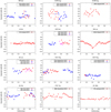 |
Fig. 1 Measured EWs of the residual Hα emission line profile of all observed objects versus orbital phase. |
3.1 Short-term variations in the chromospheric activity
The measured EWs, representing the apparent chromospheric activity level, are plotted in Fig. 1 as a function of the orbital phases (ϕ). In the residual spectra, Hα profiles show emission in almost every case, and therefore the measured EWs are negative. We decided to use the absolute value of these numbers because this convention better expresses the chromospheric activity level and its variation. In a few cases, Hα profiles show a net absorption in the residual spectra (therefore the measured EWs should be positive; however, because of the convention mentioned above, we handle them as negative numbers). Observations carried out on different nights are marked with different colors and symbols. Values of EW for the individual systems measured on different nights are mostly consistent with each other. Our spectroscopic phase coverage varies in the range ~ 50−100%. The observed variability of the chromospheric activity level can be categorized into three groups: (i) flat distribution – mostly constant activity level during the orbital revolution; (ii) one-peak distribution – enhanced activity level at a specific orbital phase; and (iii) two-peak distribution – enhanced activity levels at two different orbital phases. According to previous studies, enhanced chromospheric activity might be connected to spots on the surfaces of either or both components (e.g., Kaszas et al. 1998; Mitnyan et al. 2018).
The objects showing a flat distribution of the EW values are LS Del, V972 Her, V357 Peg, and HX UMa. These systems seem to have constant chromospheric activity levels during their orbital revolution. In the case of V972 Her, there seem to be some narrow peaks in the EW-phase diagram; however, these are probably caused by some inaccurate values (e.g., caused by an unsatisfactory continuum fit). Moreover, the orbital phase coverage is only ~70%, and therefore the category of this binary is uncertain.
Systems whose EW values show one-peak distribution are KR Com, V1073 Cyg, SW Lac, EX Leo, and OU Ser. These objects have an enhanced chromospheric activity level at a certain orbital phase. This might be explained by the presence of a large spot or group of spots visible on the surface of either or both components facing us at the given orbital phase. In the cases of KR Com and OU Ser, there is significant scattering in the data around the observed peak, and therefore whether or not thosepeaks are real is unclear. We note that V1073 Cyg and EX Leo might have another peak around ϕ = 0.2 and ϕ = 0.9, respectively, which is not covered by our observations.
Objects with a two-peak distribution of the EW values are V2150 Cyg, V351 Peg, and V781 Tau. These systems have enhanced chromospheric activity at two different orbital phases. This might indicate two active regions on the surface of one of the components (as in the case of e.g., VW Cep, see Mitnyan et al. 2018). For V351 Peg and V781 Tau, the two peaks are located approximately half an orbital phase from each other. This is consistent with the model of Holzwarth & Schüssler (2003), who showed that, in active close binaries, spots are most likely distributed on the opposite sides of the stars because of the presence of strong tidal forces. We note that in the case of V1073 Cyg and EX Leo, if there is also a peak which is uncovered with observations, then it is also located about half an orbital phase from the observed peak. V2150 Cyg does not follow this trend; however, it has the poorest orbital coverage ( ~50%) in our sample, and therefore its peak distribution is the most uncertain.
3.2 Correlation diagrams
After analyzing the short-term variations of the chromospheric activity levels of the individual systems, we examined the possible connections between the average chromospheric activity levels and some fundamental parameters of the stars. We also included VW Cephei in our sample, the data for which were analyzed in a similar way to in our previous paper (Mitnyan et al. 2018). However, for consistency, we re-analyzed that data set in exactly the same way as described in Sect. 2.3. Our final sample (13 stars) is still not large, but it is a significant improvement with respect to the four stars analyzed by Barden (1985). Moreover, Barden (1985) analyzed only W-type contact binaries and completely avoided A-type systems, while our sample contains almost equal numbers of both types. This means that we can perform a comprehensive analysis concerning this matter. However, the results remain preliminary and could be subject to bias by some effects such as sample selection or activity cycles. These effects could only be ruled out by significantly increasing the sample size in the future.
To create correlation diagrams, we averaged all the measured EW values of the residual Hα emission profiles for every single system in our sample. We then plotted these mean EW values with respect to several fundamental parameters of the systems in order to find possible correlations (Figs. 2–8.). The errors are given as the standard deviations of the individual EW values from the means. There are four objects (V1073 Cyg, V2150 Cyg, V351 Peg and V357 Peg) in our diagrams that do not follow the same trends as the other part of the sample. These have very common properties: they have the longest orbital periods, the smallest B− V color indices, and the smallest inverse Rossby numbers. Moreover, they all belong to the A-type contact binaries. Moreover, V357 Peg is the only one out of these four systems that shows almost zero chromospheric emission, as expected. However, the other three objects have significant emission, which is unexpected and does not fit the trend seen in the other part of the sample. We propose that, for these systems, there may be an additional source of Hα emission excess other than the chromospheric activity. These objects are marked with black crosses in Figs. 2–8 as outliers and are left out from the following discussions.
Figure 2 shows the mean chromospheric activity level (MCAL; i.e., mean EWs) versus orbital period for each system. It seems that the system with the shortest orbital period has the most active chromosphere. The activity level drops significantly towards longer orbital periods up to ~0.45 days. Both A- and W-type binaries in our sample follow this relation. We can only put stronger constraints on systems with short orbital periods ( ≲0.45 days) as these are overrepresented in our correlation diagram; further observations are needed to study systems with longer orbital periods.
Figure 3 shows MCAL versus B−V color index. The system with the highest B−V value can be seen to be the most chromospherically active and activity level decreases towards smaller B− V values. This trend continues upto B−V ≃ 0.45. Both A- and W-type systems seem to follow this trend. Objects with B− V ≲ 0.65 are better sampled, while more observations are needed in order to better populate the redder part of the correlation diagram.
In Fig. 4, MCAL is plotted versus the logarithm of the inverse Rossby number (see Appendix C for the derivation method of the Rossby numbers). A very similar trend to that of the B− V correlation diagram is seen (as expected because the value of the Rossby number is calibrated by the B− V color index), but it is more clear in this representation. Again, both types of contact binary follow the same trend.
We also analyzed the possible connection between the activity level and the temperature differences of the binary components. MCAL versus Teff values in Fig. 5 show a slight increase up to ≃200K, where they peak and then decrease back to approximately the original level. There seem to be no outstanding differences between A- and W-type systems.
In Fig. 6, MCAL is plotted against the mass ratio of the systems. A somewhat scattered but mostly flat distribution can be seen, without any clear trends. We note that there are no objects in our sample with 0.45 ≲ q ≲ 0.75, which also makes it more difficult to identify possible trends.
We also plotted MCAL versus the fill-out factors (f) of the systems. Figure 7 shows a flat distribution similar to the previous diagram (with a smaller scattering). There is also a gap in our data for 0.3 ≲ f ≲ 0.6, similarly to the case of mass ratios.
In our last correlation diagram (Fig. 8), we show MCAL versus the inclinations of the systems. This shows a scattered, but mostly flat distribution similarly to the previous two diagrams. Again, there is no significant difference between the behavior of A- and W-type systems.
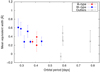 |
Fig. 2 Chromospheric activity level averaged for the whole orbital cycle versus the orbital period of the system. |
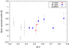 |
Fig. 3 Chromospheric activity level averaged for the whole orbital cycle versus the B− V color index of the system. |
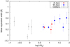 |
Fig. 4 Chromospheric activity level averaged for the whole orbital cycle versus the logarithm of the inverse Rossby-number of the system. |
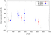 |
Fig. 5 Chromospheric activity level averaged for the whole orbital cycle versus the temperature difference of the components in the system. |
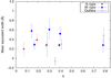 |
Fig. 6 Chromospheric activity level averaged for the whole orbital cycle versus the mass ratio of the system. |
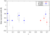 |
Fig. 7 Chromospheric activity level averaged for the whole orbital cycle versus the fill-out factor of the system. |
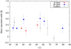 |
Fig. 8 Chromospheric activity level averaged for the whole orbital cycle versus the inclination of the system. |
4 Summary
Here, we present the results of new optical spectroscopic observations on 12 contact binary systems. Our aim is to obtain information about the short-term variations of the chromospheric activity levels and to analyze the possible connections between the mean chromospheric activity level and some fundamental stellar parameters. Based on our own spectral data set, we derived new RV curves applying the cross-correlation technique and modeled these RV curves with PHOEBE to re-determine the mass ratios and systemic velocities of the objects. Our newly derived q and Vγ values are mostly consistent with previous ones found in the literature.
In order to get constraints on the chromospheric activity level, we constructed synthetic spectra for all observed phases of the observed binaries. After that, we subtracted the model spectra from the observed ones and measured the EW values in a 10 Å wide window centered on the residual Hα line. We used these EW values as a representation of the apparent chromospheric activity strength and analyzed their variations during the orbital cycle. Regarding most of the studied systems (excluding SW Lac and HX UMa), this is the first time that any direct signs of chromospheric activity are detected. We also found different kinds of short-term variations such as continuously changing activity level with one or two peaks, or constant activity level during the whole orbital revolution. More spectra with improved S/N and temporal resolution – combined with simultaneous photometric observations – would enable a more detailed study of both short- and long-term variations of chromospheric activity.
For the purpose of searching for correlations between the chromospheric activity level and the fundamental parameters of the observed systems, we averaged all EW values of the individual systems measured in different orbital phases. After re-analyzing our data in the same way, we also included VW Cep in our sample from our previous paper (Mitnyan et al. 2018). Based on our correlation diagrams, we identify a clear connection between the mean chromospheric activity level of contact binaries and their orbital periods, their B−V color indices, and their inverse Rossby numbers. This is consistent with earlier results based on emission of the UV Mg II line (Rucinski 1985) and also those based on the analysis of optical Hα lines of a smaller sample of contact binaries (Barden 1985). We also find a possible trend on the diagram showing mean chromospheric activity level against the temperature difference of the components. Both A- and W-type systems follow these trends in a similar way. At the same time, we do not find any clear trends in MCAL versus mass ratio, fill-out factor, or the inclination of the systems.
In order to come to these conclusions, we had to exclude four objects (V1073 Cyg, V2150 Cyg, V351 Peg and V357 Peg) with very similar physical properties from the correlation analysis. We hypothesize that in these systems some other mechanism may be responsible for the observed Hα emission excess. A possible explanation could be the mass transfer between the components, which was previously proposed by Beccari et al. (2014) for some contact binaries with unusually large Hα EWs.
While our sample of contact binaries is the largest to date for which chromospheric activity has been studied using optical spectral signs, the conclusions listed above remain preliminary and should be considered with caution. The results could be biased by selection effects or magnetic activity cycles for example. A further increase in sample size is needed to efficiently rule out these effects and also to better constrain and quantify the relations found here.
Acknowledgments
We would like to thank to our anonymous referee for his/her comments which helped us to further improve the quality of this paper. This project has been supported by the Lendület grants LP2012-31 and LP2018-7/2019 of the Hungarian Academy of Sciences, by the Hungarian National Research, Development and Innovation Office, NKFIH KH-130372 grant and by the ÚNKP-18-3 New National Excellence Program of the Ministry of Human Capacities. T.M. gratefully acknowledgeobserving grant support from the Institute of Astronomy and Rozhen National Astronomical Observatory, Bulgarian Academy of Sciences. TM would like to thank to Ventsislav Dimitrov, Grigor Nikolov, Milen Minev, Lyubomir Simeonov, Mitko Churalski, Nikola Petrov and Ilian Iliev for their generous support they gave during the observations in Bulgaria.
Appendix A CCFs and radial velocity curves
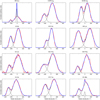 |
Fig. A.1 Sample of the derived CCFs (red) for every object close to the second quadrature (ϕ ~ 0.75) with the fitted Gaussians (black) and their sum (blue). |
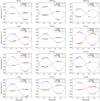 |
Fig. A.2 Radial velocity curves of every object with the fitted PHOEBE models. We note that the formal errors of the single velocity points are smaller than their symbols. |
Appendix B Sample of observed and synthetic spectra for the observed objects
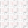 |
Fig. B.1 Sample of observed (red line) and synthesized (black line) spectra for every object at different orbital phases. |
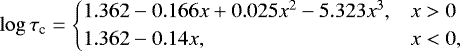
Appendix C Derivation of the Rossby numbers
The Rossby numbers were calculated as the orbital period (P) divided by the convective turnover time (τc):
 (C.1)
(C.1)
The convective turnover times were derived using the formula of Noyes et al. (1984):
 (C.2)
(C.2)
where x = 1 − (B−V ).
References
- Albayrak, B., Djurašević, G., Selam, S., et al. 2005, Ap&SS, 296, 293 [NASA ADS] [CrossRef] [Google Scholar]
- Applegate, J. H. 1992, ApJ, 385, 621 [NASA ADS] [CrossRef] [Google Scholar]
- Barden, S. C. 1985, ApJ, 295, 162 [NASA ADS] [CrossRef] [Google Scholar]
- Beccari, G., De Marchi, G., Panagia, N., & Pasquini, L. 2014, MNRAS, 437, 2621 [NASA ADS] [CrossRef] [Google Scholar]
- Binnendijk, L. 1970, Vistas Astron., 12, 217 [NASA ADS] [CrossRef] [Google Scholar]
- Blanco-Cuaresma, S. 2019, MNRAS, 486, 2075 [NASA ADS] [CrossRef] [Google Scholar]
- Blanco-Cuaresma, S., Soubiran, C., Heiter, U., & Jofré, P. 2014, A&A, 569, A111 [NASA ADS] [CrossRef] [EDP Sciences] [Google Scholar]
- Bonev, T., Markov, H., Tomov, T., et al. 2017, Bulg. Astron. J., 26, 67 [Google Scholar]
- Cereda, L., Misto, A., Niarchos, P. G., & Poretti, E. 1988, A&AS, 76, 255 [NASA ADS] [Google Scholar]
- Cruddace, R. G., & Dupree, A. K. 1984, ApJ, 277, 263 [NASA ADS] [CrossRef] [Google Scholar]
- Csizmadia, S., & Klagyivik, P. 2004, A&A, 426, 1001 [NASA ADS] [CrossRef] [EDP Sciences] [Google Scholar]
- Deb, S., & Singh, H. P. 2011, MNRAS, 412, 1787 [NASA ADS] [CrossRef] [Google Scholar]
- Demircan, O., Selam, S., & Derman, E. 1991, Ap&SS, 186, 57 [NASA ADS] [CrossRef] [Google Scholar]
- Derman, E., Demircan, O., & Selam, S. 1991, A&AS, 90, 301 [NASA ADS] [Google Scholar]
- Eggleton, P. P., & Kiseleva-Eggleton, L. 2001, ApJ, 562, 1012 [NASA ADS] [CrossRef] [Google Scholar]
- Ekmekçi, F., Elmaslı, A., Yılmaz, M., et al. 2012, New Astron., 17, 603 [NASA ADS] [CrossRef] [Google Scholar]
- Gazeas, K. D., Baran, A., Niarchos, P., et al. 2005, Acta Astron., 55, 123 [NASA ADS] [Google Scholar]
- Gray, R. O., & Corbally, C. J. 1994, AJ, 107, 742 [NASA ADS] [CrossRef] [Google Scholar]
- Grevesse, N., Asplund, M., & Sauval, A. J. 2007, Space Sci. Rev., 130, 105 [Google Scholar]
- Gustafsson, B., Edvardsson, B., Eriksson, K., et al. 2008, A&A, 486, 951 [NASA ADS] [CrossRef] [EDP Sciences] [Google Scholar]
- Hartmann, L., Baliunas, S. L., Duncan, D. K., & Noyes, R. W. 1984, ApJ, 279, 778 [NASA ADS] [CrossRef] [Google Scholar]
- Hendry, P. D., & Mochnacki, S. W. 1998, ApJ, 504, 978 [NASA ADS] [CrossRef] [Google Scholar]
- Holzwarth, V., & Schüssler, M. 2003, A&A, 405, 303 [NASA ADS] [CrossRef] [EDP Sciences] [Google Scholar]
- Kallrath, J., Milone, E. F., Breinhorst, R. A., et al. 2006, A&A, 452, 959 [NASA ADS] [CrossRef] [EDP Sciences] [Google Scholar]
- Kaszas, G., Vinko, J., Szatmary, K., et al. 1998, A&A, 331, 231 [NASA ADS] [Google Scholar]
- Kiraga, M. 2012, Acta Astron., 62, 67 [NASA ADS] [Google Scholar]
- Kjurkchieva, D., & Marchev, D. 2010, ASP Conf. Ser., 435, 111 [NASA ADS] [Google Scholar]
- Kreiner, J. M. 2004, Acta Astron., 54, 207 [NASA ADS] [Google Scholar]
- Kreiner, J. M., Rucinski, S. M., Zola, S., et al. 2003, A&A, 412, 465 [NASA ADS] [CrossRef] [EDP Sciences] [Google Scholar]
- Lanza, A. F., & Rodonò, M. 2004, Astron. Nachr., 325, 393 [NASA ADS] [CrossRef] [Google Scholar]
- Li, K., Gao, D. Y., Hu, S. M., et al. 2016, Ap&SS, 361, 63 [NASA ADS] [CrossRef] [Google Scholar]
- Lu, W., & Rucinski, S. M. 1999, AJ, 118, 515 [NASA ADS] [CrossRef] [Google Scholar]
- Lu, W., Rucinski, S. M., & Ogłoza, W. 2001, AJ, 122, 402 [NASA ADS] [CrossRef] [Google Scholar]
- Lucy, L. B. 1968, ApJ, 151, 1123 [NASA ADS] [CrossRef] [Google Scholar]
- Lucy, L. B., & Wilson, R. E. 1979, ApJ, 231, 502 [NASA ADS] [CrossRef] [Google Scholar]
- McGale, P. A., Pye, J. P., & Hodgkin, S. T. 1996, MNRAS, 280, 627 [NASA ADS] [Google Scholar]
- Mitnyan, T., Bódi, A., Szalai, T., et al. 2018, A&A, 612, A91 [NASA ADS] [CrossRef] [EDP Sciences] [Google Scholar]
- Montes, D., Fernández-Figueroa, M. J., De Castro, E., et al. 2000, A&AS, 146, 103 [NASA ADS] [CrossRef] [EDP Sciences] [Google Scholar]
- Mullan, D. J. 1975, ApJ, 198, 563 [NASA ADS] [CrossRef] [Google Scholar]
- Noyes, R. W., Hartmann, L. W., Baliunas, S. L., Duncan, D. K., & Vaughan, A. H. 1984, ApJ, 279, 763 [NASA ADS] [CrossRef] [Google Scholar]
- Pribulla, T., & Rucinski, S. M. 2006, AJ, 131, 2986 [NASA ADS] [CrossRef] [Google Scholar]
- Pribulla, T., & Vanko, M. 2002, Contrib. Astrono. Observ. Skalnate Pleso, 32, 79 [NASA ADS] [Google Scholar]
- Pribulla, T., Chochol, D., Vanko, M., & Parimucha, S. 2002, IBVS, 5258, 1 [NASA ADS] [Google Scholar]
- Pribulla, T., Rucinski, S. M., Lu, W., et al. 2006, AJ, 132, 769 [NASA ADS] [CrossRef] [Google Scholar]
- Prša, A., & Zwitter, T. 2005, ApJ, 628, 426 [NASA ADS] [CrossRef] [Google Scholar]
- Ruciński, S. M. 1973, Acta Astron., 23, 79 [NASA ADS] [Google Scholar]
- Rucinski, S. M. 1985, MNRAS, 215, 615 [NASA ADS] [CrossRef] [Google Scholar]
- Rucinski, S. M., Lu, W., & Mochnacki, S. W. 2000, AJ, 120, 1133 [NASA ADS] [CrossRef] [Google Scholar]
- Rucinski, S. M., Lu, W., Mochnacki, S. W., Ogłoza, W., & Stachowski, G. 2001, AJ, 122, 1974 [NASA ADS] [CrossRef] [Google Scholar]
- Rucinski, S. M., Lu, W., Capobianco, C. C., et al. 2002, AJ, 124, 1738 [NASA ADS] [CrossRef] [Google Scholar]
- Rucinski, S. M., Capobianco, C. C., Lu, W., et al. 2003, AJ, 125, 3258 [NASA ADS] [CrossRef] [Google Scholar]
- Rucinski, S. M., Pribulla, T., & van Kerkwijk, M. H. 2007, AJ, 134, 2353 [NASA ADS] [CrossRef] [Google Scholar]
- Rucinski, S. M., Pribulla, T., Mochnacki, S. W., et al. 2008, AJ, 136, 586 [NASA ADS] [CrossRef] [Google Scholar]
- Selam, S. O. 2004, A&A, 416, 1097 [NASA ADS] [CrossRef] [EDP Sciences] [Google Scholar]
- Selam, S., Albayrak, B., Yilmaz, M., et al. 2005, Ap&SS, 296, 305 [NASA ADS] [CrossRef] [Google Scholar]
- Selam, S. O., Esmer, E. M., Şenavcı, H. V., et al. 2018, Ap&SS, 363, 34 [NASA ADS] [CrossRef] [Google Scholar]
- Şenavcı, H. V., Hussain, G. A. J., O’Neal, D., & Barnes, J. R. 2011, A&A, 529, A11 [NASA ADS] [CrossRef] [EDP Sciences] [Google Scholar]
- Stȩpień, K., Schmitt, J. H. M. M., & Voges, W. 2001, A&A, 370, 157 [NASA ADS] [CrossRef] [EDP Sciences] [Google Scholar]
- Szczygieł, D. M., Socrates, A., Paczyński, B., Pojmański, G., & Pilecki, B. 2008, Acta Astron., 58, 405 [NASA ADS] [Google Scholar]
- Tian, X.-M., Zhu, L.-Y., Qian, S.-B., Li, L.-J., & Jiang, L.-Q. 2018, Res. Astron. Astrophys., 18, 020 [NASA ADS] [CrossRef] [Google Scholar]
- Vilhu, O. 1984, A&A, 133, 117 [NASA ADS] [Google Scholar]
- Xing, L. F., Zhang, X. B., & Wei, J. Y. 2007, New Astron., 12, 346 [NASA ADS] [CrossRef] [Google Scholar]
- Yang, Y., & Liu, Q. 2000, Ap&SS, 274, 799 [NASA ADS] [CrossRef] [Google Scholar]
- Yesilyaprak, C. 2002, IBVS, 5330, 1 [NASA ADS] [Google Scholar]
- Yuan, J., & Şenavci, H. V. 2014, MNRAS, 439, 878 [NASA ADS] [CrossRef] [Google Scholar]
- Zasche, P., & Uhlář, R. 2010, A&A, 519, A78 [NASA ADS] [CrossRef] [EDP Sciences] [Google Scholar]
- Zola, S., Gazeas, K., Kreiner, J. M., et al. 2010, MNRAS, 408, 464 [NASA ADS] [CrossRef] [Google Scholar]
Image Reduction and Analysis Facility: http://iraf.noao.edu.
All Tables
Parameters determined from radial velocity curve modeling and comparison of the derived and published (M1 + M2) sin3i values.
All Figures
|
Fig. 1 Measured EWs of the residual Hα emission line profile of all observed objects versus orbital phase. |
| In the text | |
|
Fig. 2 Chromospheric activity level averaged for the whole orbital cycle versus the orbital period of the system. |
| In the text | |
|
Fig. 3 Chromospheric activity level averaged for the whole orbital cycle versus the B− V color index of the system. |
| In the text | |
|
Fig. 4 Chromospheric activity level averaged for the whole orbital cycle versus the logarithm of the inverse Rossby-number of the system. |
| In the text | |
|
Fig. 5 Chromospheric activity level averaged for the whole orbital cycle versus the temperature difference of the components in the system. |
| In the text | |
|
Fig. 6 Chromospheric activity level averaged for the whole orbital cycle versus the mass ratio of the system. |
| In the text | |
|
Fig. 7 Chromospheric activity level averaged for the whole orbital cycle versus the fill-out factor of the system. |
| In the text | |
|
Fig. 8 Chromospheric activity level averaged for the whole orbital cycle versus the inclination of the system. |
| In the text | |
|
Fig. A.1 Sample of the derived CCFs (red) for every object close to the second quadrature (ϕ ~ 0.75) with the fitted Gaussians (black) and their sum (blue). |
| In the text | |
|
Fig. A.2 Radial velocity curves of every object with the fitted PHOEBE models. We note that the formal errors of the single velocity points are smaller than their symbols. |
| In the text | |
|
Fig. B.1 Sample of observed (red line) and synthesized (black line) spectra for every object at different orbital phases. |
| In the text | |
Current usage metrics show cumulative count of Article Views (full-text article views including HTML views, PDF and ePub downloads, according to the available data) and Abstracts Views on Vision4Press platform.
Data correspond to usage on the plateform after 2015. The current usage metrics is available 48-96 hours after online publication and is updated daily on week days.
Initial download of the metrics may take a while.