| Issue |
A&A
Volume 635, March 2020
|
|
|---|---|---|
| Article Number | A70 | |
| Number of page(s) | 6 | |
| Section | Atomic, molecular, and nuclear data | |
| DOI | https://doi.org/10.1051/0004-6361/201937088 | |
| Published online | 09 March 2020 | |
Plasma-environment effects on K lines of astrophysical interest
III. IPs, K thresholds, radiative rates, and Auger widths in Fe IX – Fe XVI⋆
1
Physique Atomique et Astrophysique, Université de Mons – UMONS, 7000 Mons, Belgium
e-mail: This email address is being protected from spambots. You need JavaScript enabled to view it.
2
Department of Physics, Western Michigan University, Kalamazoo, MI 49008, USA
3
Helmholtz Institut Jena, 07743 Jena, Germany
4
Theoretisch Physikalisches Institut, Friedrich Schiller Universität Jena, 07743 Jena, Germany
5
Cahill Center for Astronomy and Astrophysics, California Institute of Technology, Pasadena, CA 91125, USA
6
Dr. Karl Remeis-Observatory and Erlangen Centre for Astroparticle Physics, Sternwartstr. 7, 96049 Bamberg, Germany
7
NASA Goddard Space Flight Center, Code 662, Greenbelt, MD 20771, USA
8
IPNAS, Université de Liège, Sart Tilman, 4000 Liège, Belgium
Received:
8
November
2019
Accepted:
29
January
2020
Abstract
Aims. In the context of black-hole accretion disks, we aim to compute the plasma-environment effects on the atomic parameters used to model the decay of K-vacancy states in moderately charged iron ions, namely Fe IX – Fe XVI.
Methods. We used the fully relativistic multiconfiguration Dirac–Fock method approximating the plasma electron–nucleus and electron–electron screenings with a time-averaged Debye–Hückel potential.
Results. We report modified ionization potentials, K-threshold energies, wavelengths, radiative emission rates, and Auger widths for plasmas characterized by electron temperatures and densities in the ranges 105−107 K and 1018−1022 cm−3.
Conclusions. This study confirms that the high-resolution X-ray spectrometers onboard the future XRISM and Athena space missions will be capable of detecting the lowering of the K edges of these ions due to the extreme plasma conditions occurring in accretion disks around compact objects.
Key words: black hole physics / plasmas / atomic data / X-rays: general
Full Tables 4 and 5 are only available at the CDS via anonymous ftp to cdsarc.u-strasbg.fr (130.79.128.5) or via http://cdsarc.u-strasbg.fr/viz-bin/cat/J/A+A/635/A70
© ESO 2020
1. Introduction
The present paper is the third in a series devoted to density effects on atomic parameters used to model K-vacancy states in ions of astrophysical interest; namely, ionization potentials, K thresholds, transition wavelengths, radiative emission rates, and Auger widths. Deprince et al. (2019a, hereafter Paper I) computed such data for the oxygen isonuclear sequence and Deprince et al. (2019b, hereafter Paper II) did so for highly ionized Fe ions (Fe XVII – Fe XXV) using the relativistic multiconfiguration Dirac–Fock (MCDF) method (Grant et al. 1980; McKenzie et al. 1980; Grant 1988), as implemented in the GRASP92 (Parpia et al. 1996) and RATIP (Fritzsche 2012) atomic structure packages. The plasma electron–nucleus and electron–electron shielding were approximated with a time-averaged Debye–Hückel (DH) potential. Here we report our calculations using this method for the third-row Fe ions, Fe IX – Fe XVI.
The absorption and emission of high-energy photons occur in the dense plasma (1021−1022 cm−3) of the inner region of the accretion disks associated with compact objects, such as black holes and neutron stars. The modeling of the associated X-ray spectra, which can be observed with space telescopes such as Chandra, XMM-Newton, Suzaku, and NuSTAR, gives a measure of the composition, temperature, and degree of ionization for the plasma (Ross & Fabian 2005; García & Kallman 2010). For a black hole, for instance, the distortion of the Fe K lines by the strong relativistic effects constrains its angular momentum (Reynolds 2013; García et al. 2014). However, most of the atomic data used in the modeling of K-shell processes do not take density effects into account, compromising their significance for abundance determinations beyond densities of 1018 cm−3 (Smith & Brickhouse 2014).
2. Theoretical approach
The MCDF formalism was already described in Paper I and Paper II, so in this paper, we only aim to provide brief indications of the DH modifications that were introduced to handle weakly coupled plasmas. The DH screened Dirac–Coulomb Hamiltonian (Saha & Fritzsche 2006) takes the form of
 (1)
(1)
where rij = |ri − rj| and the plasma screening parameter μ is the inverse of the Debye shielding length λD, which can be expressed in atomic units (au) as a function of the plasma electron density ne and temperature Te as
 (2)
(2)
Typical plasma conditions in black-hole accretion disks are Te ∼ 105−107 K and ne ∼ 1018−1022 cm−3 (Schnittman et al. 2013) which, for weakly coupled plasmas correspond to screening parameters of 0.0 ≤ μ ≤ 0.24 au, and, for a completely ionized hydrogen plasma (plasma ionization Z* = 1) correspond to plasma coupling parameters of
 (3)
(3)
with
 (4)
(4)
in the range 0.0003 ≤ Γ ≤ 0.3.
Following Paper II, the MCDF expansions for Fe IX – Fe XVI are generated using the active space method, whereby electrons from the reference configurations in Table 1 are singly and doubly excited to configurations that include n = 3 and 4s orbitals. For instance, the non-relativistic configuration [1s2s]3p63d4s, generated by a double electron excitation from the 1s and 2s active subshells of the reference configuration 3p6 to the 3d and 4s active orbitals, is included in the expansions of the atomic state functions (ASFs) in Fe IX. As defined in Eq. (1) of Paper II, the number of configuration state functions (CSFs) generated for the MCDF expansions of the ASFs are also given in Table 1 for each ion. We consider plasma screening parameters in the range 0.0 ≤ μ ≤ 0.25 au, the upper-limit choice corresponding to the extreme plasma conditions found in accretion disks.
Reference configurations and active orbital sets used to build up the MCDF active space by single and double electron excitations to the corresponding active orbital sets along with the number of configuration state functions (CSFs) generated for the MCDF expansions in Fe IX – Fe XVI.
3. Results and discussion
3.1. Ionization potentials and K thresholds
The computed ionization potentials (IPs) and K thresholds (EK) are given in Tables 2 and 3, respectively, for plasma screening parameter μ = 0.0, 0.1 and 0.25. The case μ = 0.1 corresponds to plasma conditions of Te = 105 K and ne = 1021 cm−3 and μ = 0.25 au to Te = 105 K and ne = 1022 cm−3. For the isolated ion case (μ = 0.0 au), the computed IPs are compared in Table 2 with the values quoted in the atomic database (Kramida et al. 2018) at the National Institute of Standards and Technology (NIST), showing an agreement within 0.1%.
Computed ionization potentials for Fe IX – Fe XVI as a function of the plasma screening parameter μ (au).
Computed K-thresholds for Fe IX – Fe XVI as a function of the plasma screening parameter μ (au).
Tables 2 and 3 also show the IP and K-threshold lowering by the plasma environment at μ = 0.1 au and μ = 0.25 au: the IP downshifts are, respectively, 9–10% and 21–25%, while those for the K thresholds, due to their much larger energy, only 0.4–0.6% and 1%. Moreover, in agreement with Paper II, the absolute IP and K-threshold downshifts for each species are practically similar in magnitude. This effect can be further appreciated in Figs. 1 and 2, where we plot the absolute downshifts as a function of the effective charge, Zeff = Z − N + 1 where Z and N are respectively the atomic and electron numbers of the ionic system. We also include in these figures the Fe species with 25 ≤ Zeff ≤ 17 from Paper II and the Debye–Hückel limit ΔIPDH = −Zeff μ (Stewart & Pyatt 1966; Crowley 2014).
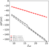 |
Fig. 1. Ionization potential shifts, ΔIP, in Fe IX – Fe XXV as a function of the effective charge Zeff = Z − N + 1. Red open circles: μ = 0.1 au. Black open circles: μ = 0.25 au. Open triangles: Debye–Hückel limit ΔIPDH = −Zeff μ. |
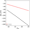 |
Fig. 2. K-threshold shifts, ΔEK, in Fe IX – Fe XXV as a function of the effective charge Zeff = Z − N + 1. Red open circles: μ = 0.1 au. Black open circles: μ = 0.25 au. |
The linear lowerings of both the IP and K threshold, ΔIP and ΔEK, respectively, with Zeff and their close magnitude for each ion are hereby reiterated. We also verify that the Debye–Hückel limit is a good approximation of the IP lowering except for two discontinuities at Zeff = 17 and 25 conspicuous at the higher plasma screening parameter (μ = 0.25), which are caused respectively by the closing of the L and K shells. It can be seen in Fig. 3 that the IP increases linearly with Zeff but two large escalations, namely a factor of 2.6 and 4, occur respectively for the closed L- and K-shell species Fe XVII and Fe XXV. The behavior of the K threshold with effective charge is somewhat different (see Fig. 4); although it still increases linearly, the gradient becomes steeper at Zeff = 17 and no effect is appreciable at Zeff = 25 since the K-shell electron is located deeper close to the nucleus in contrast to the relatively weakly bound valence electron.
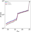 |
Fig. 3. Ionization potential, IP, in Fe IX – Fe XXV as a function of the effective charge Zeff = Z − N + 1. Blue open circles: μ = 0 au (isolated atom case). Red open circles: μ = 0.1 au. Black open circles: μ = 0.25 au. Green open stars: NIST (Kramida et al. 2018). |
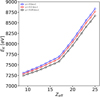 |
Fig. 4. K thresholds, EK, in Fe IX – Fe XXV as a function of the effective charge Zeff = Z − N + 1. Blue open circles: μ = 0 au (isolated atom case). Red open circles: μ = 0.1 au. Black open circles: μ = 0.25 au. |
3.2. Radiative transitions
The present MCDF K-line wavelengths are in excellent agreement with those obtained with the pseudo-relativistic Hartree–Fock (HFR) method by Palmeri et al. (2003) and Mendoza et al. (2004), differing on average by less than 0.1%, and the dispersion of the radiative transition probabilities is not larger than 20%. Regarding plasma effects, in Table 4, we tabulate the wavelengths and A-values for the stronger K lines (Aki ≥ 1013 s−1) at μ = 0, 0.1, and 0.25 au, where it can be seen that they are hardly modified redshifted by ∼1−2 mÅ or less and the radiative rates only vary by a few percent in most cases (15–20% in a handful of transitions).
Wavelengths and transition probabilities for the K lines of Fe IX – Fe XVI (9 ≤ Zeff ≤ 16) computed with plasma screening parameters μ = 0.0, 0.1, and 0.25 au.
In Fig. 5, we plot the wavelength shifts as a function of the ionic effective charge 9 ≤ Zeff ≤ 25 for μ = 0.1 and 0.25 au, again including the data from Paper II for Fe XVII – Fe XXV. We do not see a well-defined trend with Zeff, but for Zeff ≤ 17, the Kβ redshifts at μ = 0.25 au are found to be ∼2 mÅ; that is, a factor of 2 larger than the Kα lines.
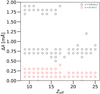 |
Fig. 5. Wavelength shifts, Δλ, for K lines in Fe IX – Fe XXV as a function of the effective charge Zeff = Z − N + 1. Red circles: μ = 0.1 au. Black circles: μ = 0.25 au. |
3.3. Auger widths
The Auger widths for the K-vacancy states we computed for the isolated atom are in good agreement with those obtained by Palmeri et al. (2003) and Mendoza et al. (2004), differences being no large than 10–15%. Similarly to the radiative rates, our Auger widths are only weakly modified by the plasma environment (see Table 5), with the reductions at μ = 0.25 au no greater than a few percent (<3%) with respect to the isolated atom.
Plasma environment effects on the Auger widths of K-vacancy states in Fe IX – Fe XVI (9 ≤ Zeff ≤ 16) computed with plasma screening parameters μ = 0.0, 0.1, and 0.25 au.
4. Summary and conclusions
Following our previous work on the oxygen isonuclear sequence (Paper I) and on the highly charged iron ions (Paper II), we studied the influence of the plasma environment on the atomic structure and on the radiative and Auger parameters associated with the K lines of the moderately charged species Fe IX – Fe XVI. The IPs, K-thresholds, wavelengths, radiative transition probabilities, and Auger widths have been calculated with the MCDF method, which includes a Debye–Hückel potential to model the plasma screening effects. To simulate the plasma conditions in compact-object accretion disks, we varied the plasma screening parameter μ from 0 au to 0.25 au. Our main results are summarized as follows.
-
We confirmed the linear redshifts of both the IP and K threshold with the effective ionic charge and their close magnitude for each species. Their values range between −20 eV to −100 eV.
-
The radiative and Auger rates are only marginally modified by the plasma environment (by a few percent overall).
-
The transition wavelengths are redshifted by less than 1 mÅ, but for the most extreme conditions studied (μ = 0.25 au), the more sensitive Kβ lines are shifted to the red by about −2 mÅ.
As discussed in the context of the highly ionized Fe ions (Paper II), the high-density plasma effects presented here are expected to have a noticeable impact on the modeling of astrophysical environments where the temperature and density reach high enough values. A prime example is the material in accretion disks formed around compact objects such as white dwarfs, neutron stars, and black holes. The standard α-disk model (Shakura & Sunyaev 1973) predicts densities in the mid-plane of the disk of order ∼1013−1027 cm−3 for black holes with masses in the range 10−109 M⊙ and reasonable values of the accretion rate and viscosity. Recent simulations based on general relativity and magnetic hydrodynamics tend to agree with the orders of magnitude of these predictions, with lower mass objects having larger densities (e.g., Schnittman et al. 2013; Jiang et al. 2019a). Accreting black holes are observed to typically emit large amounts of X-rays with a fraction of this flux reprocessed in the disk itself. This reprocessing produces a rich spectrum of fluorescence lines and other atomic features commonly described as the X-ray reflection spectrum (Ross & Fabian 2005; García & Kallman 2010). The ubiquitousness of these signatures has made X-ray reflection spectroscopy a common and powerful technique for obtaining physical information regarding the composition and ionization state of the accretion flow and the coveted black-hole spin (Fabian et al. 1989; Reynolds 2019). Due to their abundance and comparatively large fluorescence yield, along with their crucial role in determining the ionization structure of the gas producing most of the reprocessed signal, the iron ionic species featured in this paper are of particular interest for reflection modeling (García et al. 2013).
The high-quality observational data available in the last decade have revealed a number of important issues in the spectral modeling of accreting black holes; for instance, the modeling of the so-called “soft excess” in the spectrum active galactic nuclei (AGN). This is a broad and featureless component observed at soft X-ray energies (∼1 keV), which can also be described as such by several physically distinct models. As was recently demonstrated for the Seyfert 1 AGN Mrk 509 (García et al. 2019), one such model is based on the X-ray reflection spectrum from a very dense accretion disk. Higher disk densities lead to a strong excess of the reflected continuum at soft energies due to the enhancement of free–free heating in the atmosphere of the disk, which increases with rising density (Ballantyne 2004; García et al. 2016). An extended study of 17 AGN characterized by a strong soft excess have made use of high-density reflection models to reproduce their X-ray spectra (Jiang et al. 2019b), finding tentative correlations between the black-hole mass, accretion rate, and accretion-disk density.
In the study of accreting sources, the nominal values of some of the parameters obtained in reflection modeling are also relevant: in particular, the iron abundance is commonly found to be larger than the expected Solar value by factors of two up to ten (García et al. 2018). This trend is found in accreting black holes with very different masses suggesting an artificial origin rather than a physical overabundance. Reflection calculations at densities higher than the traditionally assumed values (∼1015 cm−3) have shown promise in addressing both issues. Recent analyses of the reflection spectra from AGN and black-hole binaries (BHB) appear to indicate that the high-density effects are acting positively to resolve the mystery of the high iron abundances leading to substantially lower observed values (Tomsick et al. 2018; Jiang et al. 2019b,c).
The plasma environment effects presented here have not yet been included in the studies described above. However, they are expected to affect further the atomic features imprinted in the reflection spectra and, consequently, to modify the quantities deduced from the fits. Even though a comprehensive analysis of the propagation of plasma effects in synthetic spectra is outside the scope of the present work, our conclusions suggest that some of the spectral profiles observed in the X-ray reflected spectrum from accreting sources may be modified to an extent that could potentially influence their characterization. This will be relevant for the next generation of X-ray observatories such as XRISM (Tashiro et al. 2018) and Athena (Nandra et al. 2013), which will provide an enhanced effective area in the X-ray band and instrumentation with far superior spectral resolution (of the order of a few eV) to aid in the detection of the lowering of the ionic K edges in extreme plasma conditions.
Acknowledgments
JD is Research Fellow of the Belgian Fund for Research Training in Industry and Agriculture (FRIA) while PP and PQ are, respectively, Research Associate and Research Director of the Belgian Fund for Scientific Research (F.R.S.-FNRS). Financial supports from these organizations, as well as from the NASA Astrophysics Research and Analysis Program (grant 80NSSC17K0345) are gratefully acknowledged. JAG acknowledges support from the Alexander von Humboldt Foundation.
References
- Ballantyne, D. R. 2004, MNRAS, 351, 57 [NASA ADS] [CrossRef] [Google Scholar]
- Crowley, B. J. B. 2014, High Energy Dens. Phys., 13, 84 [Google Scholar]
- Deprince, J., Bautista, M. A., Fritzsche, S., et al. 2019a, A&A, 624, A74 [NASA ADS] [CrossRef] [EDP Sciences] [Google Scholar]
- Deprince, J., Bautista, M. A., Fritzsche, S., et al. 2019b, A&A, 626, A83 [NASA ADS] [CrossRef] [EDP Sciences] [Google Scholar]
- Fabian, A. C., Rees, M. J., Stella, L., & White, N. E. 1989, MNRAS, 238, 729 [NASA ADS] [CrossRef] [Google Scholar]
- Fritzsche, S. 2012, Comput. Phys. Commun., 183, 1523 [NASA ADS] [CrossRef] [Google Scholar]
- García, J., & Kallman, T. R. 2010, ApJ, 718, 695 [NASA ADS] [CrossRef] [Google Scholar]
- García, J., Dauser, T., Reynolds, C. S., et al. 2013, ApJ, 768, 146 [NASA ADS] [CrossRef] [Google Scholar]
- García, J., Dauser, T., Lohfink, A., et al. 2014, ApJ, 782, 76 [NASA ADS] [CrossRef] [Google Scholar]
- García, J. A., Grinberg, V., Steiner, J. F., et al. 2016, ApJ, 819, 76 [NASA ADS] [CrossRef] [Google Scholar]
- García, J. A., Kallman, T. R., Bautista, M., et al. 2018, ASP Conf. Ser., 515, 282 [NASA ADS] [Google Scholar]
- García, J. A., Kara, E., Walton, D., et al. 2019, ApJ, 871, 88 [NASA ADS] [CrossRef] [Google Scholar]
- Grant, I. P. 1988, Comput. Chem., 2, 1 [Google Scholar]
- Grant, I. P., McKenzie, B. J., Norrington, P. H., Mayers, D. F., & Pyper, N. C. 1980, Comput. Phys. Commun., 21, 207 [NASA ADS] [CrossRef] [Google Scholar]
- Jiang, Y.-F., Blaes, O., Stone, J. M., & Davis, S. W. 2019a, ApJ, 885, 144 [NASA ADS] [CrossRef] [Google Scholar]
- Jiang, J., Fabian, A. C., Dauer, T., et al. 2019b, MNRAS, 489, 3436 [CrossRef] [Google Scholar]
- Jiang, J., Fabian, A. C., Wang, J., et al. 2019c, MNRAS, 484, 1972 [NASA ADS] [CrossRef] [Google Scholar]
- Kramida, A., Ralchenko, Yu., Reader, J., & NIST ASD Team 2018, NIST Atomic Spectra Database (version 5.6.1). Available: http://physics.nist.gov/asd[2019, February 1]. National Institute of Standards and Technology, Gaithersburg, MD [Google Scholar]
- McKenzie, B. J., Grant, I. P., & Norrington, P. H. 1980, Comput. Phys. Commun., 21, 233 [NASA ADS] [CrossRef] [Google Scholar]
- Mendoza, C., Kallman, T. R., Bautista, M. A., & Palmeri, P. 2004, A&A, 414, 377 [NASA ADS] [CrossRef] [EDP Sciences] [Google Scholar]
- Nandra, K., Barret, D., Barcons, X., et al. 2013, ArXiv e-prints [arXiv:1306.2307] [Google Scholar]
- Palmeri, P., Mendoza, C., Kallman, T. R., Bautista, M. A., & Meléndez, M. 2003, A&A, 410, 359 [NASA ADS] [CrossRef] [EDP Sciences] [Google Scholar]
- Parpia, F. A., Fischer, C. F., & Grant, I. P. 1996, Comput. Phys. Commun., 94, 249 [NASA ADS] [CrossRef] [Google Scholar]
- Reynolds, C. S. 2013, Classical Quantum Gravity, 30, 244004 [NASA ADS] [CrossRef] [Google Scholar]
- Reynolds, C. S. 2019, Nat. Astron., 3, 41 [NASA ADS] [CrossRef] [Google Scholar]
- Ross, R. R., & Fabian, A. C. 2005, MNRAS, 358, 211 [Google Scholar]
- Saha, B., & Fritzsche, S. 2006, Phys. Rev. E, 73, 036405 [NASA ADS] [CrossRef] [Google Scholar]
- Schnittman, J. D., Krolik, J. H., & Noble, S. C. 2013, ApJ, 769, 156 [NASA ADS] [CrossRef] [Google Scholar]
- Shakura, N. I., & Sunyaev, R. A. 1973, A&A, 24, 337 [NASA ADS] [Google Scholar]
- Smith, R. K., & Brickhouse, N. S. 2014, Adv. At. Mol. Opt. Phys., 63, 271 [NASA ADS] [CrossRef] [Google Scholar]
- Stewart, J. C., & Pyatt, Jr., K. D. 1966, ApJ, 144, 1203 [NASA ADS] [CrossRef] [Google Scholar]
- Tashiro, M., Maejima, H., Toda, K., et al. 2018, SPIE Conf. Ser., 10699, 1069922 [Google Scholar]
- Tomsick, J. A., Parker, M. L., García, J. A., et al. 2018, ApJ, 855, 3 [NASA ADS] [CrossRef] [Google Scholar]
All Tables
Reference configurations and active orbital sets used to build up the MCDF active space by single and double electron excitations to the corresponding active orbital sets along with the number of configuration state functions (CSFs) generated for the MCDF expansions in Fe IX – Fe XVI.
Computed ionization potentials for Fe IX – Fe XVI as a function of the plasma screening parameter μ (au).
Computed K-thresholds for Fe IX – Fe XVI as a function of the plasma screening parameter μ (au).
Wavelengths and transition probabilities for the K lines of Fe IX – Fe XVI (9 ≤ Zeff ≤ 16) computed with plasma screening parameters μ = 0.0, 0.1, and 0.25 au.
Plasma environment effects on the Auger widths of K-vacancy states in Fe IX – Fe XVI (9 ≤ Zeff ≤ 16) computed with plasma screening parameters μ = 0.0, 0.1, and 0.25 au.
All Figures
|
Fig. 1. Ionization potential shifts, ΔIP, in Fe IX – Fe XXV as a function of the effective charge Zeff = Z − N + 1. Red open circles: μ = 0.1 au. Black open circles: μ = 0.25 au. Open triangles: Debye–Hückel limit ΔIPDH = −Zeff μ. |
| In the text | |
|
Fig. 2. K-threshold shifts, ΔEK, in Fe IX – Fe XXV as a function of the effective charge Zeff = Z − N + 1. Red open circles: μ = 0.1 au. Black open circles: μ = 0.25 au. |
| In the text | |
|
Fig. 3. Ionization potential, IP, in Fe IX – Fe XXV as a function of the effective charge Zeff = Z − N + 1. Blue open circles: μ = 0 au (isolated atom case). Red open circles: μ = 0.1 au. Black open circles: μ = 0.25 au. Green open stars: NIST (Kramida et al. 2018). |
| In the text | |
|
Fig. 4. K thresholds, EK, in Fe IX – Fe XXV as a function of the effective charge Zeff = Z − N + 1. Blue open circles: μ = 0 au (isolated atom case). Red open circles: μ = 0.1 au. Black open circles: μ = 0.25 au. |
| In the text | |
|
Fig. 5. Wavelength shifts, Δλ, for K lines in Fe IX – Fe XXV as a function of the effective charge Zeff = Z − N + 1. Red circles: μ = 0.1 au. Black circles: μ = 0.25 au. |
| In the text | |
Current usage metrics show cumulative count of Article Views (full-text article views including HTML views, PDF and ePub downloads, according to the available data) and Abstracts Views on Vision4Press platform.
Data correspond to usage on the plateform after 2015. The current usage metrics is available 48-96 hours after online publication and is updated daily on week days.
Initial download of the metrics may take a while.