| Issue |
A&A
Volume 633, January 2020
|
|
|---|---|---|
| Article Number | A166 | |
| Number of page(s) | 7 | |
| Section | The Sun | |
| DOI | https://doi.org/10.1051/0004-6361/201937064 | |
| Published online | 28 January 2020 | |
Highly Alfvénic slow solar wind at 0.3 au during a solar minimum: Helios insights for Parker Solar Probe and Solar Orbiter
1
ASI – Italian Space Agency, via del Politecnico snc, 00133 Rome, Italy
e-mail: This email address is being protected from spambots. You need JavaScript enabled to view it.
2
National Institute for Astrophysics, Institute for Space Astrophysics and Planetology, Via del Fosso del Cavaliere 100, 00133 Roma, Italy
3
LESIA, Observatoire de Paris, Université PSL, CNRS, Sorbonne Université, Univ. Paris Diderot, Sorbonne Paris Cité, Place Jules Janssen, 92195 Meudon, France
4
Department of Physics, Imperial College London, London SW7 2AZ, UK
5
Mullard Space Science Laboratory, University College London, Dorking, UK
Received:
5
November
2019
Accepted:
13
December
2019
Abstract
Alfvénic fluctuations in solar wind are an intrinsic property of fast streams, while slow intervals typically have a very low degree of Alfvénicity, with much more variable parameters. However, sometimes a slow wind can be highly Alfvénic. Here we compare three different regimes of solar wind, in terms of Alfvénic content and spectral properties, during a minimum phase of the solar activity and at 0.3 au. We show that fast and Alfvénic slow intervals share some common characteristics. This would suggest a similar solar origin, with the latter coming from over-expanded magnetic field lines, in agreement with observations at 1 au and at the maximum of the solar cycle. Due to the Alfvénic nature of the fluctuations in both fast and Alfvénic slow winds, we observe a well-defined correlation between the flow speed and the angle between magnetic field vector and radial direction. The high level of Alfvénicity is also responsible of intermittent enhancements (i.e. spikes), in plasma speed. Moreover, only for the Alfvénic intervals do we observe a break between the inertial range and large scales, on about the timescale typical of the Alfvénic fluctuations and where the magnetic fluctuations saturate, limited by the magnitude of the local magnetic field. In agreement with this, we recover a characteristic low-frequency 1/f scaling, as expected for fluctuations that are scale-independent. This work is directly relevant for the next solar missions, Parker Solar Probe and Solar Orbiter. One of the goals of these two missions is to study the origin and evolution of slow solar wind. In particular, Parker Solar Probe will give information about the Alfvénic slow wind in the unexplored region much closer to the Sun and Solar Orbiter will allow us to connect the observed physics to the source of the plasma.
Key words: Sun: corona / Sun: heliosphere / solar wind / turbulence / plasmas
© ESO 2020
1. Introduction
The distribution of the solar-wind speed, during solar minima, shows a well-defined bimodal structure (McGregor et al. 2011). Near the Earth the distribution of the equatorial solar wind is characterised by a statistically large slow component, peaking between 350 and 400 km s−1, and a statistically smaller fast component, peaking at around 650 km s−1. The bimodal structure is even more pronounced close to the Sun, as observed at the perihelion of the Helios mission, with a separate peak at ∼650 km s−1 for the fast component. This shape, with distinct peaks rather than a smooth transition, suggests the presence of two types of wind, namely fast and slow solar wind, which are characterised by different flavours, from large-scale structures to small-scale features. In particular, slow wind shows lower proton temperature, higher density, and much more variable properties with respect to fast wind (Lopez & Freeman 1986; Schwenn 2007). The composition, anti-correlated with the speed, is another difference (Geiss et al. 1995; Kasper et al. 2012). The thermodynamics of electrons, protons, and heavy ions (mainly alpha particles) is also very different (Marsch et al. 1982a,b; Neugebauer et al. 1996; Hellinger et al. 2006; Kasper et al. 2008; Maruca et al. 2012, 2013; Matteini et al. 2013; Stansby et al. 2019a).
Another important aspect that differs in slow and fast winds is the turbulence behaviour. Independently of the speed, solar wind magnetic fluctuations show a typical Kolmogorov-like spectrum (Kolmogorov 1941) in the inertial range of the turbulent cascade (Bruno & Carbone 2013); on larger scales the two wind components are characterised by a different scaling. On the one hand, on these large scales the magnetic field spectrum of the fast wind is characterised by a 1/f scaling. The origin of this scaling is still under debate (Matthaeus & Goldstein 1986; Velli et al. 1989; Dmitruk & Matthaeus 2007; Verdini et al. 2012; Chandran 2018; Matteini et al. 2018; Tsurutani et al. 2018), but it probably corresponds to the large-scale energy in the eddies able to feed the turbulent cascade. During the solar wind expansion, the break between the large scales and the inertial range, which corresponds to the correlation length, moves to even larger scales (Matthaeus & Goldstein 1982; Bruno & Dobrowolny 1986; Horbury et al. 1996), thus corresponding to an increase in the correlation length. On the other hand, in the slow solar wind no evidence of the 1/f regime is usually recovered (Bruno & Carbone 2013) and no radial evolution is found, suggesting that the turbulence is already fully developed close to the Sun (Marsch & Tu 1990) and the correlation length is on larger scales with respect to fast wind. Very recently, for the first time, the existence of the 1/f magnetic spectral scaling has been shown also in the slow solar wind, provided that the interval is long enough to properly capture the low-frequency spectral properties (Bruno et al. 2019).
The differences between the two types of wind can be understood by looking at the regions on the Sun where the wind originates since the solar source should set its main properties. It is generally accepted that fast solar wind comes from coronal holes (Hundhausen 1972; Geiss et al. 1995), whose streams are characterised by strong anisotropic proton distribution functions, with the presence of a field-aligned beam (Marsch et al. 1982b), and large amplitude Alfvénic fluctuations (Belcher & Davis 1971). Conversely, the sources of slow solar wind are still under debate (see Abbo et al. 2016, and references therein). During the minimum of the solar activity, slow solar wind is usually observed close to the heliospheric current sheet (Smith et al. 1978) emanating from solar streamers. Conversely, during a solar maximum the structure of the corona is very complex, with no large polar coronal holes and the presence of streamers and smaller coronal holes at all latitudes. Therefore, in this case, the slow wind is not even spatially localised around the heliospheric current sheet (McComas et al. 2001). In the near future, thanks to the new solar missions, it will be possible to make several steps forward to link sources on the Sun and solar wind plasma, especially for slow streams. On the one hand, Parker Solar Probe (PSP, Fox et al. 2016), launched in August 2018, is collecting measurements in completely unexplored regions close to the Sun; on the other hand, Solar Orbiter (Muller & Marsden 2013), expected launch in 2020 February, will combine both remote sensing and in situ measurements.
Although the standard classification of fast and slow wind based on the average proton speed is widely accepted, it cannot always justify the observations. In fact, Marsch et al. (1981) observed at 0.3 au a portion of slow wind with, apart from the speed, the same characteristics of fast wind, namely significant proton-alpha drift speed, proton core temperature anisotropy, and a high degree of Alfvénicity. Moreover, Roberts et al. (1987) found the highest correlation in terms of Alfvénic fluctuations in slow solar wind. During a maximum of the solar activity, Alfvénic slow wind was observed for the first time at 1 au (D’Amicis et al. 2011) and was extensively studied with respect to large-scale properties, micro-scale phenomena, and the impact on spectral features (D’Amicis & Bruno 2015; D’Amicis et al. 2019a). The Alfvénic slow wind shares common characteristics with the fast wind, which suggests that they could have similar origin: coronal holes (D’Amicis & Bruno 2015). More recently, a thorough analysis of the Alfvénic slow wind was performed during a minimum of the solar activity in the inner heliosphere, supporting the theory that Alfvénic slow wind originates in open field lines rooted in coronal holes, where the differences with fast wind, for example the speed, could be explained by a different magnetic field geometry in the lower corona (Stansby et al. 2019b, 2020). Moreover, with respect to the measurements within an ascending phase of the solar cycle described in Marsch et al. (1981), the Alfvénic slow wind observed in a solar minimum by Stansby et al. (2019b, 2020) shows almost isotropic proton distribution functions, as in the non-Alfvénic slow wind.
The present paper complements the work done by Stansby et al. (2019b, 2020), extending the analysis to areas that were not covered. In particular, by focusing on the first perihelion of the Helios mission during a minimum phase of the solar activity, in this paper we investigate and compare the characteristics of solar wind at about 0.3 au in terms of Alfvénic content, amplitude level of fluctuations, and spectral properties in different wind regimes. The implications of our observations for PSP and Solar Orbiter are also discussed.
2. Solar wind observations
We use 40 s cadence reprocessed particle data from the Helios mission (Stansby 2017; Stansby et al. 2018), where only the core of the proton distribution function is considered. Magnetic field data are also provided as an average from the values taken whilst the distribution function was measured. An overview of the considered time interval, at the first perihelion of Helios1 in 1975, is summarised in Fig. 1. This interval corresponds to a minimum of solar activity, characterised by a series of high-speed streams separated by slower moving plasma (see panel a where the radial velocity component is shown).
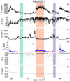 |
Fig. 1. Overview of solar wind data at the perihelion of Helios1 in 1975. (a) Radial component of the velocity; (b) radial component of the magnetic field; (c) proton density; (d) proton temperature: T∥ (red dashed line) and T⊥ (blue solid line); (e) absolute value of the 30 min averaged cross-helicity; (f) radial distance. The coloured bands denote the three different regimes of solar wind, namely Alfvénic slow (green), fast (orange), and non-Alfvénic slow (violet) winds. |
In order to classify the solar wind in Alfvénic and non-Alfvénic intervals, we compute the normalised cross-helicity defined as (Bruno & Carbone 2013)
 (1)
(1)
and evaluated in the same manner as in Stansby et al. (2019b). Here, v = vp − vp0 are the proton velocity fluctuations in the Alfvén wave frame, where vp0 is chosen to maximise the value of |σc| (Sonnerup et al. 1987), and b = VA(B/|B|) is the magnetic field in velocity units (VA being the Alfvén speed). Moreover, ⟨ ⋯⟩ denotes a time average over all points in non-overlapping 30 min windows, which corresponds to a timescale typical of Alfvénic fluctuations (Tu & Marsch 1995). The absolute value of the cross-helicity is shown in panel (e) of Fig. 1, where |σc|∼1 indicates predominantly unidirectional Alfvén waves, while |σc|< 1 indicates non-Alfvénic periods. As expected, we find that the high-speed coronal-hole plasma (Perrone et al. 2019), observed at about 0.3 au (orange band), is characterised by |σc|∼1. The same conclusion is reached by looking at the anti-correlation between the radial components of proton velocity, Vr (panel a), and magnetic field, Br (panel b). However, a very high and constant value of Alfvénicity, |σc| ∼ 0.92, is also found in a slow wind interval before perihelion (green band), associated with a similar anti-correlation between Vr and Br observed in fast solar wind. After perihelion, we observe a typical interval of slow wind (violet band), where |σc| is widely distributed between 0 and 1 and no correlation or anti-correlation is observed between Vr and Br. On March 18 at 13:46 UT, just before the beginning of the typical selected slow wind, Helios1 crossed a shock (Volkmer & Neubauer 1985), confirmed by the abrupt increase in np (panel c) and Tp (panel d) and also in the magnitude of the velocity and magnetic fields (not shown here). Therefore, we decided to remove it from our analysis.
The typical parameters, averaged within each individual selected interval, of the three different regimes of solar wind considered in this study (Alfvénic slow, fast, and non-Alfvénic slow winds) are listed in Table 1. The Alfvénic slow wind has a similar proton temperature and speed with respect to the typical non-Alfvénic slow wind. The protons in the fast wind are strongly anisotropic; instead, within Alfvénic and non-Alfvénic slow intervals the protons are almost isotropic, in agreement with the results described in Stansby et al. (2019b) but not with the measurements during an ascending phase of the solar cycle (Marsch et al. 1981) where the proton core in the Alfvénic slow wind is also anisotropic, as is the fast wind. Conversely, if during the Alfvénic slow interval the profile of proton density is almost constant, as in the case of fast wind but at a higher value, the density in typical slow wind is more variable, suggesting a more compressive nature of this plasma.
Three different regimes of solar wind used in this study, observed during the first perihelion by Helios1.
The high level of Alfvénicity produces a strong dependence of the flow speed on the angle between the magnetic field vector and the radial direction (Matteini et al. 2014, 2015). Figure 2 shows such a linear dependence for Alfvénic slow wind and for fast wind, quantified through the Pearson correlation coefficient, Rp. For the Alfvénic slow and fast intervals we find −0.68 and −0.73, respectively. Data are well aligned on a straight line, which can be described as
 (2)
(2)
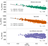 |
Fig. 2. Dependence of the solar wind speed on the local magnetic field orientation for Alfvénic slow (a), fast (b), and non-Alfvénic slow (c) winds. Rp refers to the Pearson correlation coefficient. |
where m (i.e. the slope) corresponds to the phase velocity of the Alfvénic fluctuations plus a correction due to the presence of residual energy in the plasma. Thus,  , where RA is the Alfvén ratio, defined as the ratio between the kinetic and magnetic energy per unit mass, ev/eb (Bruno & Carbone 2013). For the fast stream RA = 0.97 and VA = 168.2 km s−1, giving m = 165.3 km s−1, which should be compared with the slope of the fit (i.e. |m| = 163.2 km s−1). We note that RA ∼ 1, which means there is equipartition of energy between velocity and magnetic field fluctuations, as expected for a pure Alfvén wave (Alfvén 1942). A good agreement is also found for the Alfvénic slow wind, where RA = 0.56 and VA = 75.8 km s−1 give m = 56.8 km s−1, which should be compared with |m| = 45.1 km s−1. In this case, RA < 1, meaning that some power is also in non-Alfvénic modes. On the other hand, no linear correlation is expected for the non-Alfvénic slow wind. This is confirmed by panel (c) of Fig. 2 where the points are substantially more scattered; thus, the Pearson correlation coefficient is about zero (Rp = 0.04). Moreover, for this interval RA = 0.38, meaning that the energy in magnetic field fluctuations dominates the energy in velocity fluctuations, probably due to variations of density and magnetic field magnitude.
Another important characteristic observed in fast streams is the presence of spikes (Horbury et al. 2018; Perrone et al. 2019), or anti-Sunward propagating Alfvénic fluctuations. They look like intermittent enhancements in plasma speed, whose contribution is more important in regions close to the Sun since their amplitude decreases as the plasma moves away from the Sun (Matteini et al. 2014; Perrone et al. 2019). A statistical analysis at 0.3 au has shown that these spikes can last seconds to minutes and can recur on scales of minutes to tens of minutes (Horbury et al. 2018). Figure 3 shows the probability distribution function (PDF) of the instantaneous radial velocity fluctuations with respect to a 30 min running mean, δv = Vr − ⟨Vr⟩, normalised to the mean value in the considered stream of the Alfvén speed, VA, for fast (orange solid line), Alfvénic slow (green-dashed line), and non-Alfvénic slow (violet dash-dotted line) winds. The normalisation allows us to quantitatively compare the different streams, since the amplitude of the spikes is constrained by VA due to their Alfvénic nature (Matteini et al. 2015). As expected (Horbury et al. 2018; Perrone et al. 2019), the distribution of δv/VA for the fast wind is characterised by a long right tail (positively skewed with γ ≃ 1.5). Moreover, we observe the presence of spikes also in the Alfvénic slow stream, where the skewness is positive (γ ≃ 2.1, greater than in the case of fast wind), even if the amplitude of the Alfvénic fluctuations is lower with respect to fast wind. On the other hand, the distribution of δv/VA in non-Alfvénic slow wind, due to its non-Alfvénic nature, does not show any presence of spikes and the distribution is more symmetric (γ ≃ 0.9) and narrower with respect to the Alfvénic intervals.
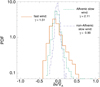 |
Fig. 3. Probability distribution function of the radial speed with respect to a 30 min running mean, normalised to the mean value in each considered stream of the Alfvén speed, for fast (orange solid line), Alfvénic slow (green dashed line), and non-Alfvénic slow (violet dash-dotted line) winds. γ refers to the value of the skewness of each distribution. |
3. Spectral properties
Velocity and magnetic field fluctuations in the solar wind exhibit characteristic turbulence power spectra for both the fast and slow streams (Bruno & Carbone 2013). The differences are recovered on larger scales where a robust 1/f scaling range is typically observed in fast (Alfvénic) wind. Figure 4 shows the total power density spectrum (i.e. the trace of the spectral matrix) of the magnetic field and velocity field fluctuations for Alfvénic slow, fast, and non-Alfvénic slow solar wind, normalised to the square value of the mean field intensity in each interval. The 1/f scaling on a large scale and the Kolmogorov expectation in the inertial range have been included for reference. For both magnetic and velocity fluctuations, we observe that the power level is higher for fast wind than for slow wind. In particular we find that the power level decreases moving from fast to Alfvénic slow to non-Alfvénic wind. However, the differences in amplitude are more pronounced for the velocity field with respect to the magnetic field. The same behaviour, with a higher power level for fast wind, is observed for both magnetic and velocity non-normalised spectra (not shown). However, in the latter, Alfvénic and non-Alfvénic streams present almost the same level of fluctuations. It is worth noting that in order to follow the behaviour of the fluctuations from large scales to the MHD regime, we use magnetic field observations at 4 Hz (Musmann et al. 1975), a much better resolution with respect to the plasma parameters (∼40 s). Unfortunately, for velocity fluctuations only large scales can be studied and no information for the inertial range is available.
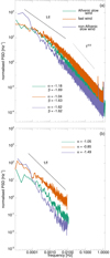 |
Fig. 4. Normalised power spectral density (PSD) of total magnetic (a) and velocity (b) fluctuations. The 1/f scaling (black solid lines) and the Kolmogorov expectation (black dotted line) have been plotted for reference. |
By looking in detail at the magnetic fluctuations (panel a), we find a clear spectral break between the injection range and the inertial range of the turbulent cascade in the fast stream (orange), located at ∼10−3 Hz, a typical timescale for Alfvénic fluctuations (D’Amicis et al. 2019a). The spectral indices for the injection scales, in the frequency range f ∈ [10−4, 2 × 10⁻³] Hz, and for the inertial range, in the frequency range f ∈ [0.02, 0.2] Hz, are α = −1.04 ± 0.04 and β = −1.631 ± 0.006, respectively. Therefore, the spectral break clearly separates the 1/f region and the typical f−5/3 Kolmogorov fully developed turbulence. A similar behaviour, albeit less clear, is also recovered for the Alfvénic slow wind (green), where the spectral indices for the injection and inertial ranges are α = −1.18 ± 0.11 (for f ∈ [10−4, 10−3] Hz) and β = −1.686 ± 0.009, respectively. On the other hand, completely different spectral properties are found for the non-Alfvénic wind (violet), where the Kolmogorov inertial range extends to all observed frequencies and there is no evidence of a low-frequency spectral break. The spectral indices for the injection and inertial ranges are the same: α = −1.62 ± 0.05 (for f ∈ [10−4, 4 × 10⁻³] Hz) and β = −1.62 ± 0.01, respectively. These results, at 0.3 au and during a minimum of the phase of the solar activity, are in agreement with the observations at 1 au and during a maximum of the solar cycle (D’Amicis et al. 2019b).
Another difference between Alfvénic and non-Alfvénic wind can be observed in the behaviour of the velocity fluctuations (panel b). On the one hand, Alfvénic wind, both fast and Alfvénic slow intervals, shows the 1/f low-frequency range, as in the case of magnetic fluctuations, where the strong correlation of the two field is due to the Alfvénic nature of the fluctuations. In particular, we find α = −0.85 ± 0.05 and α = −1.05 ± 0.12 for the fast and Alfvénic slow wind, respectively. On the other hand, for the non-Alfvénic slow wind, we find α = −1.49 ± 0.05, comparable with the value of the Iroshnikov–Kraichnam scaling of 3/2, in agreement with Podesta et al. (2006), among others, and more recently confirmed by D’Amicis et al. (2019b). Therefore, for the non-Alfvénic slow interval, there is no evidence of 1/f low-frequency range, because velocity and magnetic fluctuations are decoupled, as expected for low Alfvénicity (Bruno et al. 2019).
The presence of the 1/f low-frequency range in the Alfvénic intervals, for scales larger than the correlation length, could be due to the saturation of the amplitude of the magnetic fluctuations, whose average value reaches the mean magnetic field magnitude (Matteini et al. 2018). By using measurements at 4 Hz for the magnetic field, we define the fluctuations at scale Δt as the magnitude of δB(t, Δt) = B(t) − B(t + Δt). Following the study of Matteini et al. (2018), the time increments are evaluated using 17 logarithmically spaced lags, Δt, from 1 to 2 × 10⁵ s, in order to cover the full inertial range and the 1/f low-frequency range. However, due to the short duration of the slow intervals, we can cover with good statistics only until ∼4 × 10⁴ s, which is still enough to describe the transition from the MHD range to the 1/f scaling. Therefore, in order to have a remarkable comparison between the fast and slow intervals, in our analysis we consider only 15 time increments for each stream.
The left panels of Fig. 5 show the PDFs of δB/B for fast (top), Alfvénic slow (middle), and non-Alfvénic slow (bottom) intervals, where the vertical dotted lines refer to δB/B = 2. In the case of low magnetic compressibility (i.e. the magnetic field remains constant in time and at different scales), the maximum amplitude of the difference between two magnetic field vectors is twice the approximately constant radius of the sphere where the tip of the magnetic field vectors is forced to move, as a geometrical consequence of the Alfvénic nature of the fluctuations (see e.g. Bruno et al. 2004; Matteini et al. 2015). For both fast and Alfvénic slow wind, we observe a very clear cutoff in the distributions at δB/B = 2, where the populated left part of the PDFs represents the main incompressible component of the turbulence. On the other hand, the PDFs related to kinetic scales (from light green to red) becomes narrower, due to the presence of small rotations of the magnetic field vector (Chen et al. 2015), and gradually populate the region for δB/B > 2. We also observe that the PDFs do not evolve further on large scales, for Δt > 103 s, and they lie approximately on top of each other, in agreement with the fact that in the 1/f range the amplitude of fluctuations becomes independent of the considered scale. A different behaviour is observed for the non-Alfvénic slow wind, where the PDFs continuously evolve from large to small scales, meaning that no saturation is recovered and no 1/f range is observed at low frequency. Moreover, the right side of the PDFs is more populated with respect to the case of Alfvénic winds, due to a significant change in the modulus of the magnetic field, eventually related to compressive events (Perrone et al. 2016).
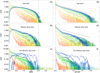 |
Fig. 5. Probability distribution function of δB/B (left column) and δB2/2B2 (right column), for fast (top row), Alfvénic slow (middle row), and non-Alfvénic slow (bottom row) winds. Left panels: vertical dotted lines refer to δB/B = 2. In panels d and e, the dashed lines display the exponential dependence of δB2/2B2 on the cosine of the rotation angle ϕ. The time increments are evaluated using 15 logarithmically spaced lags, Δt, from 1 s (red lines) to ∼4 × 10⁴ s (blue lines). |
The right panels of Fig. 5 show the PDF of δB2/2B2, which is linked to the rotation angle, ϕ, between two magnetic field vectors as δB2/2B2 ∼ 1 − cos ϕ, for pure rotations in a range [0, 2] (Zhdankin et al. 2012; Matteini et al. 2018). For both fast (top panel) and Alfvénic slow (middle panel) winds, we observe that when moving from small to large scales the distributions of δB2/2B2, and thus of cosϕ, become flatter meaning that the fluctuations tend to cover the full sphere. However, the distributions never become completely flat, suggesting that the fluctuations, even on the largest scales, are not completely uncorrelated, but they keep memory of the mean field direction. The saturation level of the PDFs is shown by dashed lines in panels (d) and (e), which refer to an exponential dependence of δB2/2B2 on the cosine of the rotation angle ϕ, as ∼e−ξ(1 − cos ϕ), where ξ = 2.1 is an empirical constant evaluated for the fast stream. Very different is the behaviour of the non-Alfvénic interval (bottom panel), whose PDFs do not show any clear dependence on ϕ and no saturation is found. It is worth noting that the slope of cosϕ for Alfvénic winds is much steeper (ξ = 2.1) compared to the value observed for Ulysses magnetic field measurements, during a solar minimum, but at radial distances of 1.4 − 2.2 au and heliographic latitudinal variation from 30° to 80° (Matteini et al. 2018). In the latter case, the empirical constant ξ is close to unity (ξ = 0.8). However, our result is consistent with other Helios fast wind observations at 0.3 au, where ξ ∼ 1.8 (Matteini et al. 2019). This could suggest some evolution with distance, where the distribution of angles spread out on the sphere with R, and then ξ would be related to the level δB/B.
Figure 6 shows the average value of δB/B for each PDF in Fig. 5 for fast (red triangles), Alfvénic slow (green stars), and non-Alfvénic slow (violet circles) winds. The average ratio ⟨δB/B⟩ corresponds to the normalised first-order structure function and is linked to the spectral slopes of the power density spectrum. In particular, if l = 1/k is a physical scale, δB ∝ l1/3 corresponds to the spectral index −5/3 observed in the inertial range of the turbulent spectrum, while δB = const corresponds to the spectral index −1 observed on large scales for the Alfvénic winds. For fast and Alfvénic slow winds, we find, for Δt < 103 s, that ⟨δB/B⟩ increases as l1/3 and then, for Δt > 103 s, that ⟨δB/B⟩ saturates at about 1, corresponding to the 1/f low-frequency range in the turbulent spectrum (see panel a of Fig. 4). However, the value at which ⟨δB/B⟩ saturates for the two intervals is different, because the amplitude of fluctuations is larger for fast wind with respect to Alfvénic wind. In particular, ⟨δB/B⟩ ∼ 0.8 for fast wind (red triangles) and ⟨δB/B⟩ ∼ 0.6 for Alfvénic slow wind (green stars). Conversely, no saturation is found for the non-Alfvénic slow wind, since the spectrum is not characterised by a 1/f range, and ⟨δB/B⟩ continuously increases in the considered range of scales.
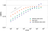 |
Fig. 6. Average value of δB/B from inertial to large scales, for fast (red triangles), Alfvénic slow (green stars), and non-Alfvénic slow (violet circles) winds. |
4. Discussion and conclusions
We have presented a detailed comparison between three different regimes of solar wind at ∼0.3 au, during a minimum phase of the solar activity, by using magnetic field and reprocessed proton-core Helios data. The selection of the intervals was focused on several parameters. In particular, we chose a fast solar wind interval composed only of unperturbed plasma from a coronal hole (Perrone et al. 2019), thus avoiding the interaction regions always present at the edges of high-speed streams, which represent an external source of compression and heating. The cross-helicity evaluated at the first perihelion of the mission confirms, as expected, the strong Alfvénic nature of the fluctuations in fast wind with respect to typical slow wind, which is indeed characterised by a low degree of Alfvénicity. On the other hand, we identified another interval with a low speed, typical of slow wind, but where the Alfvénicity is high, as in fast wind.
The first evidence of an Alfvénic slow wind was found at 0.3 au during an ascending phase of the solar cycle (Marsch et al. 1981), when the properties of the solar wind are substantially different with respect to those at the solar minimum. Moreover, no detailed characterisation was performed for this slow wind at that time. More recently, Alfvénic slow wind has been observed at 1 au during the maximum of the solar activity, and thoroughly studied also in comparison with fast and typical slow solar wind (D’Amicis & Bruno 2015; D’Amicis et al. 2019a). Only recently has Alfvénic slow wind been identified during a minimum of the solar activity and in the inner heliosphere (Stansby et al. 2019b, 2020), but no analysis of the spectral characteristics has been presented. Therefore, for the first time, here we address the spectral properties of Alfvénic slow wind during a minimum of the solar cycle and close to the Sun.
We find that Alfvénic slow wind at 0.3 au has the same low speed observed for the non-Alfvénic slow wind, and the proton temperature is also comparable (with the Alfvénic slow interval a bit hotter), which is much lower than that of the fast stream (see Table 1). Moreover, both slow winds are characterised by an isotropic proton distribution function, while in fast solar wind the protons are strongly anisotropic in the perpendicular direction with respect to the magnetic field (Stansby et al. 2019b, 2020). For the density and magnetic field magnitude, the Alfvénic slow wind is similar to the fast wind, both characterised by lower and almost constant values with respect to the non-Alfvénic slow wind, which instead shows a higher magnetic and plasma compression. These observations in the inner heliosphere and at a minimum of the solar cycle are almost in agreement with the measurements at 1 au and at a maximum of the solar activity (D’Amicis et al. 2019a). This suggests that the characteristics of Alfvénic slow wind are set by the solar source of this wind, probably from overexpanded coronal holes (D’Amicis & Bruno 2015; Stansby et al. 2020), and do not change, with respect to the fast and non-Alfvénic winds, during the radial evolution of the plasma, at least above the Alfvén point. In this context, Parker Solar Probe will play a crucial role in giving information about the Alfvénic slow wind in the unexplored region much closer to the Sun. However, we expect that PSP will recover, far from the Alfvén point, the same characteristics observed by Helios and Wind. Moreover, thanks to Solar Orbiter, it will be possible to explore the link between solar sources and plasma properties, thus eventually confirming the corona-hole origin of Alfvénic slow wind.
We also observed a well-defined correlation between the proton speed and the angle between the magnetic field vector and the radial direction in both fast and Alfvénic slow wind. Conversely, the speed in the non-Alfvénic slow interval does not show any linear correlation with θBR. This is in agreement with previous studies (Matteini et al. 2014, 2015; D’Amicis et al. 2019a) where the modulation of the flow speed by the direction of the local magnetic field can be seen as a consequence of the high level of Alfvénicity. Moreover, the Alfvénic nature of the fluctuations in both fast and Alfvénic slow wind is also responsible for the presence of spikes (Horbury et al. 2018; Perrone et al. 2019) in plasma speed. Since they can reach a high speed (an important fraction of the Alfvén speed) with respect to the ambient wind, they carry a significant fraction of the total momentum and energy of the plasma (Horbury et al. 2018). PSP is predicted to have been connected to a small coronal hole during its first perihelion (Riley et al. 2019), at ∼35 R⊙, helping the analysis of spikes in a region never explored before and where their contribution could be crucial to understanding the heating of the solar wind. In fact, since the amplitude of spikes decreases as the plasma moves away from the Sun (Matteini et al. 2014; Perrone et al. 2019), in the regions close to the Sun a very important contributions at the heating could be due to these intermittent enhancements in speed. Furthermore, in the near future, Solar Orbiter, thanks to the synergy between in situ and remote sensing measurements, will provide insights into the understanding of the spikes with respect to the source of the plasma by allowing an accurate magnetic connectivity analysis.
Finally, we compared the spectral properties for the three considered regimes and we found a different turbulence behaviour between Alfvénic and non-Alfvénic winds, due to the different nature of the fluctuations. Alfvénic winds are characterised by larger amplitude power spectra with respect to the non-Alfvénic slow wind. However, in contrast to the results at 1 au and at the maximum of the solar cycle where the amplitude of the magnetic field fluctuations in the Alfvénic winds are almost the same (D’Amicis et al. 2019a,b), in the present intervals (i.e. at the minimum of the solar activity and at 0.3 au), the fast wind shows fluctuations with larger amplitude with respect to the Alfvénic slow wind, in normalised and in non-normalised values. The same differences are found for the velocity field. Moreover, for the Alfvénic intervals, we observed a break separating the inertial range from the large scales approximately on the timescale typical of the Alfvénic fluctuations, and a characteristic 1/f scaling on larger scales, as expected for fluctuations that are scale-independent, for both magnetic and velocity fields, in agreement with D’Amicis et al. (2019b). Furthermore, this spectral break corresponds to the scale on which the magnetic fluctuations saturate, limited by the magnitude of the local magnetic field, ⟨δB/B⟩≲1. It is worth pointing out that at solar minimum the 1/f range in the Alfvénic slow wind is not the same as for the fast wind and in this case the saturation level for the Alfvénic slow interval is quite low (∼0.6). This is a clear difference with the observations at 1 au and at the maximum of the solar activity (D’Amicis et al. 2019a). On the other hand, for the non-Alfvénic slow wind, the Kolmogorov inertial range extends to all frequencies and no saturation of the magnetic fluctuation is recovered. However, the absence of the low-frequency break could be explained by the length of the considered interval of the non-Alfvénic slow wind, which is not long enough to properly capture the low-frequency spectral properties (Bruno et al. 2019). PSP will be able to investigate the turbulence properties of the solar wind inside the Alfvén radius and the origin, in terms of the radial distance, of the 1/f low-frequency range. These new measurements could help us to investigate the differences between the observations at different radial distances and during different phases of the solar activity.
Acknowledgments
Work by DS and TSH was supported by STFC grant ST/N000692/1; and LM was supported by the Programme National PNST of CNRS/INSU co-funded by CNES. The authors acknowledge collaborations with the PSP and Solar Orbiter Science Team. In particular, TSH acknowledges membership in PSP FIELDS and SWEAP teams.
References
- Abbo, L., Ofman, L., Antiochos, S. K., et al. 2016, Space Sci. Rev., 201, 55 [NASA ADS] [CrossRef] [Google Scholar]
- Alfvén, H. 1942, Nature, 150, 405 [NASA ADS] [CrossRef] [Google Scholar]
- Belcher, J. W., & Davis, L. 1971, J. Geophys. Res., 76, 3534 [NASA ADS] [CrossRef] [Google Scholar]
- Bruno, R., & Carbone, V. 2013, Liv. Rev. Sol. Phys., 10, 1 [Google Scholar]
- Bruno, R., & Dobrowolny, M. 1986, Ann. Geophys., 4, 17 [NASA ADS] [Google Scholar]
- Bruno, R., Carbone, V., Primavera, L., et al. 2004, Ann. Geophys., 22, 3751 [Google Scholar]
- Bruno, R., Telloni, D., Sorriso-Valvo, L., et al. 2019, A&A, 627, A96 [NASA ADS] [CrossRef] [EDP Sciences] [Google Scholar]
- Chandran, B. D. G. 2018, J. Plasma Phys., 84, 905840106 [CrossRef] [Google Scholar]
- Chen, C. H. K., Matteini, L., Burgess, D., & Horbury, T. S. 2015, MNRAS, 453, L64 [NASA ADS] [CrossRef] [Google Scholar]
- D’Amicis, R., & Bruno, R. 2015, ApJ, 805, 84 [NASA ADS] [CrossRef] [Google Scholar]
- D’Amicis, R., Bruno, R., & Bavassano, B. 2011, J. At. Sol. Terr. Phys., 73, 653 [NASA ADS] [CrossRef] [Google Scholar]
- D’Amicis, R., Matteini, L., & Bruno, R. 2019a, MNRAS, 483, 4665 [NASA ADS] [Google Scholar]
- D’Amicis, R., Matteini, L., Bruno, R., & Velli, M. 2019b, Sol. Phys. [Google Scholar]
- Dmitruk, P., & Matthaeus, W. H. 2007, Phys. Rev. E, 76, 036305 [NASA ADS] [CrossRef] [Google Scholar]
- Fox, N. J., Velli, M., Bale, S. D., et al. 2016, Space Sci. Rev., 204, 7 [NASA ADS] [CrossRef] [Google Scholar]
- Geiss, J., Gloeckler, G., & von Steiger, R. 1995, Space Sci. Rev., 72, 49 [Google Scholar]
- Hellinger, P., Trávnícek, P. M., Kasper, J. C., & Lazarus, A. J. 2006, Geophys. Res. Lett., 33, L09101 [NASA ADS] [CrossRef] [Google Scholar]
- Horbury, T. S., Balogh, A., Forsyth, R. J., & Smith, E. J. 1996, A&A, 316, 333 [NASA ADS] [Google Scholar]
- Horbury, T. S., Matteini, L., & Stansby, D. 2018, MNRAS, 478, 1980 [NASA ADS] [CrossRef] [Google Scholar]
- Hundhausen, A. J. 1972, . Springer-Verlag, PCS, 5 [Google Scholar]
- Kasper, J. C., Lazarus, A. J., & Gary, S. P. 2008, Phys. Rev. Lett., 101, 261103 [NASA ADS] [CrossRef] [PubMed] [Google Scholar]
- Kasper, J. C., Stevens, M. L., Korreck, K. E., et al. 2012, ApJ, 745, 162 [NASA ADS] [CrossRef] [Google Scholar]
- Kolmogorov, A. N. 1941, Dokl. Akad. Nauk. SSSR, 30, 301 [NASA ADS] [Google Scholar]
- Lopez, R. E., & Freeman, J. W. 1986, J. Geophys. Res., 91, 1701 [NASA ADS] [CrossRef] [Google Scholar]
- Marsch, E., & Tu, C.-Y. 1990, J. Geophys. Res., 95, 8211 [NASA ADS] [CrossRef] [Google Scholar]
- Marsch, E., Muehlhaeuser, K.-H., Rosenbauer, H., Schwenn, R., & Denskat, K. U. 1981, J. Geophys. Res., 86, 9199 [NASA ADS] [CrossRef] [Google Scholar]
- Marsch, E., Rosenbauer, H., Schwenn, R., Muehlhaeuser, K.-H., & Neubauer, F. M. 1982a, J. Geophys. Res., 87, 35 [Google Scholar]
- Marsch, E., Schwenn, R., Rosenbauer, H., et al. 1982b, J. Geophys. Res., 87, 52 [NASA ADS] [CrossRef] [Google Scholar]
- Maruca, B. A., Kasper, J. C., & Gary, S. P. 2012, ApJ, 748, 137 [NASA ADS] [CrossRef] [Google Scholar]
- Maruca, B. A., Bale, S. D., Sorriso-Valvo, L., Kasper, J. C., & Stevens, M. L. 2013, Phys. Rev. Lett., 111, 241101 [NASA ADS] [CrossRef] [Google Scholar]
- Matteini, L., Hellinger, P., Goldstein, B. E., et al. 2013, J. Geophys. Res., 118, 2771 [Google Scholar]
- Matteini, L., Horbury, T. S., Neugebauer, M., & Goldstein, B. E. 2014, Geophys. Res. Lett., 41, 259 [Google Scholar]
- Matteini, L., Horbury, T. S., Pantellini, F., Velli, M., & Schwartz, S. J. 2015, ApJ, 802, 11 [NASA ADS] [CrossRef] [Google Scholar]
- Matteini, L., Stansby, D., Horbury, T. S., & Chen, C. H. K. 2018, ApJ, 869, L32 [NASA ADS] [CrossRef] [Google Scholar]
- Matteini, L., Stansby, D., Horbury, T. S., & Chen, C. H. K. 2019, IL Nuovo Cimento 42 C, 1, 16 [NASA ADS] [Google Scholar]
- Matthaeus, W. H., & Goldstein, M. L. 1982, J. Geophys. Res., 87, 10347 [NASA ADS] [CrossRef] [Google Scholar]
- Matthaeus, W. H., & Goldstein, M. L. 1986, Phys. Rev. Lett., 57, 495 [NASA ADS] [CrossRef] [Google Scholar]
- McComas, D. J., Goldstein, R., Gosling, J. T., & Skoug, R. M. 2001, Space Sci. Rev., 97, 99 [NASA ADS] [CrossRef] [Google Scholar]
- McGregor, S. L., Hughes, W. J., Arge, C. N., Owens, M. J., & Odstrcil, D. 2011, J. Geophys. Res., 116, A03101 [NASA ADS] [Google Scholar]
- Muller, D., Marsden, R. G., & St. Cyr, O. C., & Gilbert, H. R., 2013, Sol. Phys., 285, 25 [NASA ADS] [CrossRef] [Google Scholar]
- Musmann, G., Neubauer, F. M., Maier, A., & Lammers, E. 1975, Raumfahrtforschung, 19, 232 [NASA ADS] [Google Scholar]
- Neugebauer, M., Goldstein, B. E., Smith, E. J., & Feldman, W. C. 1996, J. Geophys. Res., 101, 17047 [NASA ADS] [CrossRef] [Google Scholar]
- Perrone, D., Alexandrova, O., Mangeney, A., et al. 2016, ApJ, 826, 196 [NASA ADS] [CrossRef] [Google Scholar]
- Perrone, D., Stansby, D., Horbury, T. S., & Matteini, L. 2019, MNRAS, 483, 3730 [Google Scholar]
- Podesta, J. J., Roberts, D. A., & Goldstein, M. L. 2006, J. Geophys. Res., 111, A10109 [NASA ADS] [CrossRef] [Google Scholar]
- Riley, P., Downs, C., Linker, J. A., et al. 2019, ApJ, 874, L15 [NASA ADS] [CrossRef] [Google Scholar]
- Roberts, D. A., Goldstein, M. L., Klein, L. W., & Matthaeus, W. H. 1987, J. Geophys. Res., 92, 12023 [NASA ADS] [CrossRef] [Google Scholar]
- Schwenn, R. 2007, Space Sci. Rev., 124, 51 [Google Scholar]
- Smith, E. J., Tsurutani, B. T., & Rosenberg, R. L. 1978, J. Geophys. Res., 83, 717 [NASA ADS] [CrossRef] [Google Scholar]
- Sonnerup, B. U. Ö., Papamastorakis, I., Paschmann, G., & Lühr, H. 1987, J. Geophys. Res., 92, 12137 [NASA ADS] [CrossRef] [Google Scholar]
- Stansby, D. 2017, https://doi.org/10.5281/zenodo.1135245 [Google Scholar]
- Stansby, D., Salem, C., Matteini, L., & Horbury, T. 2018, Sol. Phys., 293, 155 [NASA ADS] [CrossRef] [Google Scholar]
- Stansby, D., Perrone, D., Matteini, L., Horbury, T. S., & Salem, C. S. 2019a, A&A, 623, L2 [NASA ADS] [CrossRef] [EDP Sciences] [Google Scholar]
- Stansby, D., Horbury, T. S., & Matteini, L. 2019b, MNRAS, 482, 1706 [NASA ADS] [CrossRef] [Google Scholar]
- Stansby, D., Matteini, L., Horbury, T. S., et al. 2020, MNRAS, 492, 39 [NASA ADS] [CrossRef] [Google Scholar]
- Tsurutani, B. T., Lakhina, G. S., Sen, A., et al. 2018, J. Geophys. Res., 123, 2458 [CrossRef] [Google Scholar]
- Tu, C.-Y., & Marsch, E. 1995, Space Sci. Rev., 73, 1 [Google Scholar]
- Velli, M., Grappin, R., & Mangeney, A. 1989, Phys. Rev. Lett., 63, 1807 [NASA ADS] [CrossRef] [Google Scholar]
- Verdini, A., Grappin, R., Pinto, R., & Velli, M. 2012, Apj, 750, L33 [NASA ADS] [CrossRef] [Google Scholar]
- Volkmer, P. M., & Neubauer, F. M. 1985, Ann. Geophys., 3, 1 [NASA ADS] [Google Scholar]
- Zhdankin, V., Boldyrev, S., & Mason, J. 2012, ApJ, 760, L22 [NASA ADS] [CrossRef] [Google Scholar]
All Tables
Three different regimes of solar wind used in this study, observed during the first perihelion by Helios1.
All Figures
|
Fig. 1. Overview of solar wind data at the perihelion of Helios1 in 1975. (a) Radial component of the velocity; (b) radial component of the magnetic field; (c) proton density; (d) proton temperature: T∥ (red dashed line) and T⊥ (blue solid line); (e) absolute value of the 30 min averaged cross-helicity; (f) radial distance. The coloured bands denote the three different regimes of solar wind, namely Alfvénic slow (green), fast (orange), and non-Alfvénic slow (violet) winds. |
| In the text | |
|
Fig. 2. Dependence of the solar wind speed on the local magnetic field orientation for Alfvénic slow (a), fast (b), and non-Alfvénic slow (c) winds. Rp refers to the Pearson correlation coefficient. |
| In the text | |
|
Fig. 3. Probability distribution function of the radial speed with respect to a 30 min running mean, normalised to the mean value in each considered stream of the Alfvén speed, for fast (orange solid line), Alfvénic slow (green dashed line), and non-Alfvénic slow (violet dash-dotted line) winds. γ refers to the value of the skewness of each distribution. |
| In the text | |
|
Fig. 4. Normalised power spectral density (PSD) of total magnetic (a) and velocity (b) fluctuations. The 1/f scaling (black solid lines) and the Kolmogorov expectation (black dotted line) have been plotted for reference. |
| In the text | |
|
Fig. 5. Probability distribution function of δB/B (left column) and δB2/2B2 (right column), for fast (top row), Alfvénic slow (middle row), and non-Alfvénic slow (bottom row) winds. Left panels: vertical dotted lines refer to δB/B = 2. In panels d and e, the dashed lines display the exponential dependence of δB2/2B2 on the cosine of the rotation angle ϕ. The time increments are evaluated using 15 logarithmically spaced lags, Δt, from 1 s (red lines) to ∼4 × 10⁴ s (blue lines). |
| In the text | |
|
Fig. 6. Average value of δB/B from inertial to large scales, for fast (red triangles), Alfvénic slow (green stars), and non-Alfvénic slow (violet circles) winds. |
| In the text | |
Current usage metrics show cumulative count of Article Views (full-text article views including HTML views, PDF and ePub downloads, according to the available data) and Abstracts Views on Vision4Press platform.
Data correspond to usage on the plateform after 2015. The current usage metrics is available 48-96 hours after online publication and is updated daily on week days.
Initial download of the metrics may take a while.