| Issue |
A&A
Volume 633, January 2020
|
|
|---|---|---|
| Article Number | A25 | |
| Number of page(s) | 20 | |
| Section | Astrophysical processes | |
| DOI | https://doi.org/10.1051/0004-6361/201731721 | |
| Published online | 03 January 2020 | |
Radiation phenomenon for large meteoroids⋆
1
Retired, Formerly of NASA Ames Research Center, Moffet Field, CA, USA
e-mail: This email address is being protected from spambots. You need JavaScript enabled to view it.
2
Korea Advanced Institute of Science and Technology (KAIST), Daejeon, Korea
Received:
5
August
2017
Accepted:
19
June
2019
Abstract
Aims. The relationship between the intrinsic properties of a large meteoroid, that is, mass, density, chemical composition, and flight velocity, and its spectrum are identified.
Methods. Assuming thermochemical equilibrium and inviscid flow and using a quasi-one-dimensional approach, the flow-field and radiative transfer problems are solved from the ablating wall of a meteoroid to the observer on the ground.
Results. The study discovers that the precursor region immediately ahead of the shock layer absorbs nitrogen and oxygen lines, and thereby modifies the spectrum received by the ground observer. The study leads to a computer code with which the observed spectra and light-curves for Benesov and Sumava meteoroids are numerically and approximately reproduced with the help of a meteoroid fragmentation theory. Luminous efficiency value is obtained as a byproduct.
Key words: meteorites, meteors, meteoroids / radiation mechanisms: thermal / shock waves
A copy of the code is available at the CDS via anonymous ftp to cdsarc.u-strasbg.fr (130.79.128.5) or via http://cdsarc.u-strasbg.fr/viz-bin/cat/J/A+A/633/A25
© ESO 2020
1. Introduction
Entry flights of meteoroids have been observed over the ages by several different groups of people for each different reasons. Since the invention of photography and spectroscopy in the late nineteenth century, however, acquiring and studying the spectra of the radiation emitted during their atmospheric flights became one popular scientific pursuit. It is becoming even more popular of late for two reasons. First, meteoroids are known to inflict damage to the ground on impact, to a very large extent in some instances; knowing more about it may help in mitigating the damage. And second, meteoroids may have seeded life to primitive Earth (Chyba 1997). This proposition originates from the observation that most of the amino acid molecules found in meteorites are of left-handed type (for example, Glavin et al. 2012). Amino acid molecules contain an NH2 radical. There are two symmetrical positions where the radical can attach to the rest of the molecule, left or right. Depending on which side the radical attaches, they are called either left-handed or right-handed type. When amino acid molecules are synthesized in a laboratory, two types are found in equal numbers. But amino acid molecules in the living things on the Earth are of the left-handed types only, the same types as in meteoroids.
Even though many meteoroid spectra have been obtained, the relation between the spectra and the intrinsic characteristics of the meteoroids is little known. Most of the past works on this problem approached the problem from phenomenological point of view (for example, Pecina & Kolten 2009): luminous efficiency, which relates radiation phenomenon to meteoroid mechanical and thermochemical behavior, is deduced empirically (for example, Ceplecha & McCrosky 1976). One can immediately ask two questions: (1) what is the value of the luminous efficiency that relates the brightness of the meteoroid radiation to ablation rate? and (2) why many meteoroid spectra lack spectral lines of oxygen and nitrogen which should be the strongest because they are on the outside region of the radiating gas volume and are heated to the highest temperature?
In order to answer such questions, one must describe, from the first principles, meteoroid’s fluid-mechanical, thermo-chemical, and radiation behavior over the entire domain of interest, that is, from the ablating surface of the meteoroid to the ground observer. The domain of interest is illustrated schematically in Figs. 1a and b. As shown in Fig. 1a, radiation is produced by the hot region, called shock layer, between the bow-shaped shock wave, called bow shock, and the wall of the meteoroid. As radiation emerges from the bow shock wave toward the ground, it passes through a region called the precursor region. In this region, radiation is partly absorbed, which raises the local temperature and causes air to partially dissociate and ionize. The passing radiation is partially absorbed by the dissociated and ionized air. In 1969, an experiment was conducted to determine how far the precursor region extends (Omura & Presley 1969). Electrons were found 6 m ahead of the shock wave.
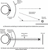 |
Fig. 1. Acquisition process of radiation emitted by a meteoroid, shown schematically. Top panel: two-dimensional depiction of the light beam path captured by the ground observer. Bottom panel: this two-dimensional light path is replaced by a horizontal line to represent the two-dimensional affair into a one-dimensional affair. |
The fluid mechanics of the flow around an object entering into Earth’s atmosphere from outer space has been studied in great detail in the past for speeds up to about 13 km s−1. Radiation was accounted for in such studies. Radiation was the main heating mechanism for the re-entering spacecraft Apollo (to the Moon, Park 2004), Pioneer-Venus (to Venus, Park & Ahn 1998), Galileo (to Jupiter, Park 2009), Stardust (to asteroid, Winter & Trumble 2011) and Hayabusa (to asteroid, Winter et al. 2012). For the Stardust and Hayabusa vehicles, radiation emitted during their entry flight was observed in much the same manner as taking meteor spectra.
There are three reasons why the meteor radiation problem is difficult and time-consuming to calculate. The first is the complexity of the physics involved. Not only that the shock layer temperature is higher than any human have faced until now but also that the predominant physics involves rather unusual thermochemical non-equilibrium and viscous mixing phenomena (Park 1990). The second is the multi-dimensionality: the flow is at least axi-symmetrically two-dimensional or fully three-dimensional. The third is having to calculate radiation line-by-line: one is uneasy about the reliability of the approximate methods such as Rosseland approximation (Park 2015).
It is the general aim of the present work to theoretically determine how the radiation phenomenon occurs for Earth-entering meteoroids. Of necessity, only the simplest case is tackled. First, the complexity of coupling of ablation processes with fragmentation processes is avoided by considering only the net ablation product, that is, the portion of the vaporized matter that leaves the liquid surface. Likewise, only the stagnation region is considered in the heating-ablating environment: the occasional occurrence of a second maximum heating point in the downstream due to turbulent transition is ignored. Thermochemical difficulties are avoided by limiting considerations only to the equilibrium cases. The shock layer flow should be in thermo-chemical equilibrium if the meteoroid is large in comparison with the mean-free path of the ambient air. Around a large meteoroid, air flow will also behave as an inviscid flow. This size limitation will limit the usefulness of the present work: large-meteor events are rare. Analysis of the small meteoroids, which would have wider applications, will have to be left for the future. The present work serves as a starting point for such a research.
Second, the multi-dimensionality is avoided by adopting a quasi-one-dimensional approach. In a shock layer flow, the quantities along the centerline can be calculated accurately through the use of a coordinate transformation devised spontaneously six decades ago by almost every leading researcher. In order to obtain the overall ablation rate or radiation intensity accurately, one needs to integrate the local ablation rate or radiation intensity values over the surface area corresponding to 0 < Θ < π/2, where Θ is the polar angle. In the present quasi-one-dimensional method, the local values are assumed to vary as cosines of the angle Θ, which should be a reasonable approximation. Under this approximation, the overall values simply become the centerline values times the frontal area πR2 of the meteoroid,  .
.
Third, line-by-line approach is kept, though one simplification is introduced. In order to faithfully reproduce the line shape, one needs about two million wavelength points Park (2013, 2015). The present simplification, to be described later, reduces the needed number of wavelength points from two million to 400 000. This line-by-line calculation method, and the necessary computer code, was developed first by NASA (Whiting et al. 1969). It had an international influence, producing several local versions. The present work uses the version developed jointly by Japan’s JAXA (Japan Aerospace Exploration Agency) and Korea’s KAIST (Korea Advanced Institute of Science and Technology) named SPRADIAN07 and currently operated by Fujita & Abe (1997), and Hyun (2009) 1. The sources of the intensity parameters of both atomic and diatomic species are given by Park (2013, 2015).
In the SPRADIAN07 code used in the present work, half-half Stark width of the atomic lines is assumed to be expressible as Arnold et al. (1979)
 (1)
(1)
The parameters α and β must be specified in the input file for atomic lines. Known values of these parameters are given in the input table. If they are left as zero, they take the default values of α = 0.042[Ep/(Ep − E)]2 and β = 0.33. Additionally, Stark widths of 77 lines were given specific values in the range from zero to 10 A. The details will have to be obtained directly from the data file, which will be open to public use.
In the last decade, significant improvement was made on treating the diatomic molecular bands. The intensity parameters in the diatomic table are up-to-date. The treatment of the rotational symmetry in a diatomic molelcule was improved (Hyun 2009): rotational branches and associated Hoenl-London factors were fully determined to triplet states and partly to quintet states (because FeO radiation is by quintet states), following the method of Kovacs (1969). Unpublished error corrections made in Kovacs’ original formulation by the late Dr. Kovacs himself and his colleague Dr. Whiting, and communicated to the present author privately, were accommodated.
The present work resulted in a Fortran f90 code named meteor-spect.f90. The code is applied to Benesov and Sumava meteoroids. The spectra and brightness calculated by the code agree with the observations for those two meteoroids.
2. Method of analysis
2.1. Flow-field
In Park (2014), fluid mechanics of the present problem are described in full. Therein, the flow-field around a meteoroid entering Earth’s atmosphere is analyzed following the traditional methodology developed in the aerospace community for the heat-shields of spacecraft entering the atmosphere. Before proceeding with the analysis, the difference between the two problems is first examined. A difference exists in that, for meteoroids, there is no backing metal plate.
Physically, a meteoroid is a porous solid body with void fraction ranging from a small value, for example 0.05, to a large value 0.90. This point is similar to spacecraft heat-shields: the heat-shield of the Apollo spacecraft (Park 2004) had a void fraction of around 0.45, and the more recent PICA (phenol-impregnated carbon ablator) had a void fraction of around 0.85 (Tran et al. 1997). One can classify meteoroids by the degree of porosity into two classes: slightly porous and highly porous.
In Fig. 2a, the ablating behavior of a slightly porous meteoroid is shown. Under the radiative heating from the hot shock layer, the surface of the meteoroid melts. The melt forms a layer covering the surface of the porous solid. The interior of a meteoroid is at a pressure lower than in the shock layer, because a meteoroid is flying in from a region of lower ambient density (higher altitude). Therefore, the porous solid tends to draw this melt into solid’s interior. However, because the porosity is small, the flow rate of the melt will be small. As soon as the melt is drawn into the porous solid, it will condense. The result is a two-layer situation, a liquid layer and a solid layer, as shown in Fig. 2a. The interface between the gaseous ablation product and the liquid layer, and the interface between the liquid layer and the solid layer both recede as ablation progresses. Through imperfections in the liquid layer, small amount of air will flow and reach the slightly porous solid, and fill and pressurize it, eventually causing it to break up.
 |
Fig. 2. Overall view of ablating meteoroid. For a slightly porous meteoroid (panel a), a layer of liquid melt forms over the solid meteoroid. For a highly porous meteoroid, (panel b), a layer of densified solid forms below the liquid layer. Air molecules pass through the holes existing in the liquid layer and the densified solid layer, eventually permeating through the porous solid. |
In Fig. 2b, ablating behavior of a highly porous meteoroid is shown. In this case, many small holes will be formed in the liquid layer through which the ablation product gas and air will pass, because of the strong suction from the highly porous solid. The liquid drawn into the solid solidifies to form a layer having average density higher than the porous solid, as shown in Fig. 2b, but having holes through which the gaseous state can pass. The ablation product will solidify in the densified solid layer, but air will pass through and reach the porous solid. The three surfaces, (1) the interface between the ablation product layer and the liquid layer, (2) the interface between the liquid layer and the densified solid layer, and (3) the interface between the densified solid layer and the porous solid layer, all recede with approximately the same speed. Inside the porous solid, air will permeate with a measurable speed and quickly increase the inside pressure to a fairly high level, causing it to break up relatively early. The densification of porous body is not unfamiliar in the aerospace community. Density of the Apollo’s heat-shield increased by a factor of about 1.5 (Park 2004) and the density of the heat-shield for Stardust (PICA) increased by a factor of about 1.8 (Stackpoole et al. 2013) in the outermost region of what is left of their heat-shields.
Air molecules that passed through the holes in the liquid layer and the densified solid layer flow through the porous interior. In the porous interior, it is driven by the favorable pressure gradient therein. Here, the air molecules permeate through the porous medium with velocity v following Darcy’s equation
 (2)
(2)
The resulting internal pressure causes the meteoroid to split and break up. The order of magnitude value of v can be obtained from the high-end value for K for loose sands (considering meteoroids to be loose aglomerates of sand grains) of 2.6 × 10⁻¹² m2 (Bear 1972), the estimated viscosity μ value at 3000 K of 1.0 × 10⁻⁵ Pa s, and dp/dy of 105 Pa m−1, to be about 3 × 10⁻³ m s−1, a very small value. A more realistic estimate of v can be made from the observed break-up periods of meteoroids. According to Park & Brown (2012), the time intervals between break-ups of meteoroids is mostly the times the air flow permeates through the meteoroids. Because these time intervals are on the order of a second, the velocity v is deduced to be about 1 m s−1 for meteoroid of 1 m in diameter. Either way, v is much smaller than the velocity of the vapor in the shock layer. Thus the traditional method of analysis of the shock layer flow around spacecraft which neglects this inward flow is valid for meteoroids.
With this assertion, one can analyze the ablation phenomenon. Only the essence will be given here because the details are given by Park (2014). As in Park (2014), the present work assumes the meteoroid to be spherical in shape. The shock layer flow is considered to consist of two layers, the air shock layer and the ablation-product vapor layer, as shown in Figs. 3a and b. One considers the control volume to be a region bound by a circular cylinder of a small radius r chosen so that
 (3)
(3)
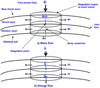 |
Fig. 3. Stagnation region flow-field of ablating meteoroid. In the frontal region of a meteoroid flying through the atmosphere, two distinct layers of gaseous state form behind the bow shock wave, one by air (shock layer) in the outer region and the other by the ablation-product (ablation layer) in the inner region. The quantities flowing axially are denoted with dots, that is, Ṁ and Q̇, and are per area per sec. The quantities flowing radially are denoted without dots, that is M and Q, and are per sec. |
The unit of length associated with rx here is immaterial. The quantities passing axially through this cylinder are represented with dots, for example Ṁ. In contrast, the radially moving quantities is represented without dots, e.g. M.
The mass flow rate of the free-stream air flow entering the cylinder is  . The mass flow rate of air leaving the cylindrical surface is
 (4)
(4)
where u is the velocity component parallel to the wall. As will be further elaborated, for a short radial distance r, u grows linearly with r so that one can write
 (5)
(5)
Using this relationship, one obtains
 (6)
(6)
Likewise, for M2, one obtains
 (7)
(7)
Equations (6) and (7) determine the thickness of the air layer and the vapor layer.
A normal coordinate  can be introduced as
 (8)
(8)
Using the hypersonic flow assumption and the assumption that the tangential velocity u varies linearly between the interface (i) and the shock (s), one obtains, for the air layer
 (9)
(9)
 (10)
(10)
Because of the continuity relationship between ρu and ρv, one has
 (11)
(11)
where
 (12)
(12)
 (13)
(13)
For the vapor layer, a function f̃ can be introduced as having the property of
 (14)
(14)
 (15)
(15)
satisfying the equation
 (16)
(16)
At the wall, (ρv)w = Ṁ, and therefore
 (17)
(17)
At the interface, v = 0, and so
 (18)
(18)
Before Eq. (16) is integrated, it is crucial to understand the behavior of its solution near the interface, as depicted in Fig. 3. For the flow of an ablation product, the flow near the interface resembles the low speed axisymmetric stagnation flow over a flat plate shown in Fig. 4. Figure 4 shows an upside-down schematization of the flow-field around the stagnation point shown in Fig. 3 for the ablation layer. The flow of ablation product blowing from the ablating wall in Fig. 3 corresponds to the uniform flow blowing from y = ∞ in Fig. 4. The stagnation point in Fig. 4 corresponds to the stagnation point on the interface in Fig. 3. The uniform flow from y = ∞ bends the direction 90° and becomes a radial flow parallel to the flat plate as shown in Fig. 4. As given in most textbooks in advanced calculus, in this flow-field, velocity is the gradient of a potential function Ψ = Axy where A is an arbitrary constant. Velocity components are u = Ax and v = Ay, that is, both the horizontal and vertical components of velocity vary linearly with the distance from the stagnation point. This behavior occurs to the ablation-product flow around the stagnation point in Fig. 3: v in the solution to Eq. (16) must approach this linear relation v = (dv/dy)y near the interface, and the tangential component u must approach u ≈ (du/dr)r near the central axis. A burden of the simplicity of this flow-field is that the stagnation point becomes a singular point if any quantity must be divided by u or v at the stagnation point.
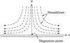 |
Fig. 4. Three-dimensional incompressible inviscid flow blowing normally against a flat plate. Radial distance is x, and vertical distance is y. Streamline and stagnation points are indicated. |
Paradoxically, numerical integration of Eq. (16) is possible only in the regions away from the interface: the interface is the singularity described above because division by v occurs in numerical integration. An approximate solution for f̃ satisfying Eqs. (17) and (18) is obtained in Park (2014) though a fifth-order polynomial expansion around the interface
 (19)
(19)
where
 (20)
(20)
![Mathematical equation: $$ \begin{aligned}&c_5 = {1\over {20\tilde{\eta }_{\rm { e}}^3}} \left[2c_2+d_2\tilde{\eta }_{\rm { e}} + \left(-{3\over 4}d_{\rm { 3}} +{1\over 2}d_2c_2\right)\tilde{\eta }_{\rm { e}}^2 - f_{\rm w}^{\prime \prime }\right]\cdot \end{aligned} $$](/articles/aa/full_html/2020/01/aa31721-17/aa31721-17-eq24.gif) (21)
(21)
Here, the parameters d2 and d3 are the coefficients in the fit
 (22)
(22)
The value of  is the solution of
 (23)
(23)
Here, f̃w″ is given by
 (24)
(24)
A fifth order fit is chosen because higher order fits diverge (Park 2014).
Equation (19) is evaluated down to a point 20% of the ηe away from the interface. A straight line is fitted from ηe to the 20% point to satisfy the linearity requirement of the solution near the interface.
Equation (16) can be seen as a part of a more thorough formulation used widely in high-speed flow studies, which involves not only the normal distance parameter  but also the tangential distance parameter
  . The equation combining the mass and momentum conservation relations is written as a power series in
  . Equation (16) is its first term, and is numerically accurate to within 1% to Θ of about 15°.
In order to assess the validity of the present inviscid flow approximation, one first determines the thickness of the viscous mixing region. To do so, one resorts to the traditional boundary layer analysis. Therein, the normalized normal coordinate is η
 (25)
(25)
The velocity field in this viscous region is expressed by a function f having the property
 (26)
(26)
The mass and momentum conservation relation corresponding to Eq. (16) is, with some simplification
 (27)
(27)
If one assumes that there are two chemical species, and there are no chemical reactions occurring in the flow-field under consideration, and the mass fraction of one species is z, then its conservation equation becomes, under some simplification (in which Schmidt number is unity),
 (28)
(28)
Simultaneous solution of Eqs. (27) and (28) shows that most (70%) of change occurs over the distance of Δη = 1. That is, the thickness of the mixing region is given by
![Mathematical equation: $$ \begin{aligned} \Delta \eta \approx 1,\;\Delta { y} \approx \left[2 {{\rho _{\rm { e}}}\over {\mu _{\rm { e}}}}\left({{\mathrm{d}u_{\rm { e}}}\over {\mathrm{d}r}}\right)\right]^{-1/2}\cdot \end{aligned} $$](/articles/aa/full_html/2020/01/aa31721-17/aa31721-17-eq36.gif) (29)
(29)
Equation (28) is a diffusion equation in the present flow-field. Because of the analogy between diffusion and heat conduction, temperature will obey it if temperature variation is only by conduction.
The magnitude of wall value of f
 (30)
(30)
is a measure of how thick the vapor layer is in comparison with the thickness of the mixing region. It is called the blowing parameter (Libby 1970). If it is substantially larger than unity, say 5, then blowing can be said to be massive, and the present inviscid approximation can be considered valid. The y-domain under consideration is represented by 200 node points, half for the vapor layer and the air layer.
2.2. Radiation spectrum
Given that the emission coefficient is related to the absorption coefficient through the Planck function, only absorption coefficients need to be calculated. The basic method of determining the absorption coefficient in the present environment is given by Park (2014). Under the inviscid-flow assumption, the elemental mass fractions in the two layers remain the same everywhere in each layer. The chemical compositions, and hence the wavelength-dependent absorption coefficients κλ, become a function only of pressure and temperature for a given chemical composition of the meteoroid.
Along the centerline, pressure can be considered constant, though, in reality, it varies by about 3%. Therefore, the absorption coefficients become a function only of temperature. The absorption coefficients can be calculated for several temperatures for the given pressure prior to the flow calculation, stored in a table, and interpolated for the needed temperature.
The equilibrium compositions are first calculated from the partition functions by solving a system of simultaneous rate equations. For atoms, all energy levels listed in the NIST atomic database are included. Up to quadruple ionized states are included for air. Up to doubly ionized states are considered for the ablation product. Lowering of ionization potential in large electron density environments and truncation of levels due to high density are not accounted for. This limits validity of the present work to relatively low-density regimes, meaning high altitudes of about 40 km. Extending the present work to lower altitudes is left for the future. Bound-free absorption cross sections for atomic species given by Peach (1978) are adopted. For those species not given by Peach, absorption cross sections are calculated from the assumed Gaunt factor values of unity.
The calculation procedure is as follows. For each given freestream density and flight velocity, centerline shock layer pressure and the post-shock equilibrium temperature are first calculated. This post-shock temperature and the wall temperature mark the limits of the temperatures for which absorption coefficient values need to be calculated. The absorption coefficients are calculated at equal intervals in the 10 000/T space and are stored. Three tables are produced. (1) For air shock layer, the upper limit of temperature is the post-shock temperature and the lower limit of temperature is taken to be 1/1.4 of the post-shock temperature. The absorption coefficients are calculated at five temperatures. (2) For the vapor layer, the upper limit is taken to be 1/2 of the post-shock temperature, and the lower limit is taken to be 2600 K. The absorption coefficients are calculated at 11 temperatures. (3) For the precursor region, absorption coefficients are calculated at 11 temperatures, starting from 1500 K.
The velocity and energy field calculation and spectrum calculation use these three tables (energy field, and hence velocity field, is affected by radiation). The three tables can be used unlimited number of times for the flow-field calculation.
In Park (2013, 2015), two-million wavelength points were used in order to calculate the Rosseland mean absorption coefficients. These many wavelength points will require computing times too large to be practical in the present work. In the present work, a trick is devised in order to reduce the needed number of wavelength points from 2 × 10⁶ to 400 000, as follows:
For bound-free and free-free continua, a coarse wavelength grid will be acceptable. A coarse wavelength grid will be a problem only for spectral lines. In the radiation code used, the wavelength of the center of a line is chosen to be that of the nearest wavelength node. Trapezoidal, that is, linear, integration is made to calculate the area under the curve. This procedure results in a small error in the wavelength of the line, but it is inconsequential. This situation is shown schematically in Fig. 5 where the solid line shape is calculated by the Voigt function, the line-shape function in the code. The correct area under the curve is the area below this curve. If the absorption coefficient value at the line center is kept as it is, and the coarse wavelength grid also is kept, the area under the curve implied in the code is that shown by the chain lines, which is larger than the correct area. In order to prevent this error, the line-center value of absorption coefficient is adjusted as
 (31)
(31)
as shown by the dash curve. This leads to an approximately correct implied area.
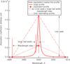 |
Fig. 5. Profile of the 5001.86 Fe I line. Abscissa is wavelength in Angstrom and ordinate is absorption coefficient in arbitrary units. Wavelength step is 9.00 A. The wavelength mesh point closest to 5001.86 A is 5000 A. |
An example is shown in Fig. 5. The wavelength of the line center is, in the coarse-grid approximation, the wavelength of the nearest node point 5000 A. The line is described by three points, first at 4991 A with zero intensity, second 5000 A with the intensity of the peak point, and the third at 5009 A with zero intensity. On the other hand, one can construct a detailed Voigt line profile centered at 5000 A. The area under the triangle defined by the three points in the coarse-grid approximation is much larger than the area under the Voigt profile. Equation (31) lowers the peak point from the line peak to a point shown by a circle, which produces a triangle containing an area approximately equal to the area under the Voigt profile.
The short wavelength limit is taken to be 1/2.5 times that of the peak in Planck function. The long wavelength limit is taken to be 2.5 times that of the Planck function peak. The wavelength intervals are made to vary linearly between the smallest and the largest values, while the largest interval is made to be twice that of the smallest interval.
The calculated spectrum is folded by an instrument function of Gaussian shape. The half width at half height of the Gaussian slit function is given as an input parameter. It was taken to be 2.5 A for most of the present work, a typical compromise between resolution and speed.
Chemical composition of the meteoroid is specified by the input data. The input data specifies the weight fractions of 14 chemical compounds: SiO2, TiO2, Al2O3, Cr2O3, Fe2O3, FeO, MgO, CaO, Na2O, H2O, Fe, Ni, FeS, and C.
As indicated in the Introduction, the radiation code developed in the present work was tested for Benesov and Sumava meteoroids, the two most prominent large meteoroids with known spectra. Because the chemical compositions of these meteoroids are unknown, they were synthesized in the present work as follows. The compositions of nine meteoroids of extreme compositions, meaning a high percentage of one or two chemical compounds, were selected from the composition table compiled by Jarosewich (1990). Then P2O5, which typically has a value of 0.0020, MnO of 0.0018, and K2O of 0.0003 were assumed not to exist: P2O5 was considered to be a part of Fe2O3, MnO as part of FeO, and K2O as part of Na2O. The remaining compounds found in these nine meteoroids were assumed to exist to concentrations equal to the largest values found among them. Next, because the sum of the percentages of these components so generated exceeds 100%, concentration values were normalized by dividing by the sum value. The concentrations values were then rounded off to produce closest whole values, while maintaining the total at 100%. This strategy was thought to have the best chance of reproducing the observed spectra of the two meteoroids, because all major components were included. As will be shown later, the synthesized chemical compositions roughly reproduce the observed spectra of Benesov and Sumava meteoroids.
The synthesized chemical composition of the two meteoroids are, by mass: SiO2 = 0.2900, TiO2 = 0.0100, Al2O3 = 0.0200, Cr2O3 = 0.0050, Fe2O3 = 0.1000, FeO = 0.0900, MgO = 0.2500, CaO = 0.0020, Na2O = 0.0090, H2O = 0.0090, Fe = 0.1480, Ni = 0.0100, FeS = 0.050, C = 0.0100. These values are also given in Table C.1.
In the vapor phase, the ablation product is considered to contain S, H, C, O, Si, Mg, Fe, Ca, Al, Na, Ti, Cr, Ni, AlO, O2, OH, CO, SO, SiO, MgO, FeO, TiO, SiO2, S+, C+, H+, O+, Si+, Mg+, Fe+, Ca+, Al+, Na+, Ti+, Cr+, Ni+, Al++, C++, S++, O++, Si++, Mg++, Fe++, Ti++, Cr++, and Ni++. The emissivity value of the ablating surface was assumed to be 0.5.
The high temperature air is considered to consist of N, N2, O, O2, NO, NO+, N+, O+,  , N++, O++, N3+, O3+, N4+, and O4+. The present chemical species makeup should be valid to up to 100 000 K of post-shock temperature, or roughly 40 km s−1 of flight speed.
2.3. Energy field
The wall temperature was determined by imposing the gas-to-condensed state equilibrium relationship for the given solid-state composition. The needed data are taken from the JANAF Thermochemical tables (Chase 1998). The details are given by Park (2014), and will not be repeated here. The wall temperature so calculated varied from 2500 K to 3500 K in the present work. The gas-surface equilibrium calculation also yields the value of the vaporization energy ΔH. The calculated ΔH value is about 17 MJ kg−1, which is a little more than half of those of the carbon-based materials used for the heat-shields of spacecraft. The effective vaporization energy is this value divided by what is defined in the present work as spallation factor described below.
Heating of the wall is assumed to be solely by radiation. The convective heat transfer rate is negligible first because radiation is so strong and second because the wall convective heat transfer rate is reduced by the ablation phenomenon by the factor roughly equal to (Libby 1970)
 (32)
(32)
which is very small for fw greater than 1. A steady-state ablation is assumed, meaning the heat transferred to the wall is balanced solely by ablation; no part of the heat is expended in raising the temperature of the interior.
But an ablating wall is known to release small particles of the body material Park (1999), Davies & Park (1983), and Park et al. (2004) in a process known as spallation. Spallation is peculiar because it does not absorb energy, or very little if any, rather energy is expended in the main action for mass removal such as radiation. One can introduce total mass removal rate ṁt and spallation factor j as
 (33)
(33)
where j is equal to or greater than unity. Because spallation is assumed not to absorb energy, continuity of energy dictates
 (34)
(34)
Arc-heated wind tunnel experiments measure Fw and mt, and deduce ΔH/j. Thus, ΔH/j is being measured, given that ΔH itself cannot be measured as spallation is inseparable.
According to the data obtained for spacecraft heat-shields, j is close to unity for dense material, and approaches 2 for loose material. No material was found so far to have a factor greater than 2. It is assumed here to be unity for the Benesov meteoroid because the meteoroid is relatively dense (55% of the ideal value), and two for the Sumava meteoroid which is loose (8% of the ideal value).
The energy conservation in the shock layer flow-field can be written symbolically as
 (35)
(35)
where ∇.F is the divergence of radiative heat flux
 (36)
(36)
But because the solution is sought only along the stagnation streamline, one has
 (37)
(37)
The radiative heat fluxes F+ and F− are calculated by integrating the intensity Iλ over wavelengths and solid angles. The intensity value Iλ is obtained in turn by solving the radiative transfer equation
 (38)
(38)
The energy Eq. (37) cannot be integrated totally numerically because ρv becomes zero at the interface. Therefore, analytical extrapolation was made with the partly numerically integrated values. Numerical integration was started from the end points and stopped at the 80% points. Then the values obtained up to that point were fit with a fourth-order polynomial. Extrapolation to the singular point was performed with the polynomial.
Equation (37) was solved iteratively. Enthalpy distribution was first assumed. From the equilibrium relationship, temperature and species concentrations were determined. From these, ϵλ and κλ were determined. Radiation intensity Iλ was calculated at ten angles separated by 9°. By carrying out solid angle integrations over these ten angles, the divergence of radiative heat flux ∇.F was calculated. Then the energy Eq. (37) was integrated as described above using the ρv values obtained from Eqs. (11) and (19) to obtain an improved enthalpy values. Using the enthalpy values so improved, the iteration process was repeated.
2.4. Precursor region
The outward-facing component of the radiation generated inside the shock layer leaves the bow shock wave and passes through the precursor region as shown schematically in Fig. 6. The normal component of the radiation and the absorption cross-section of air in the region are shown for a typical case in Fig. 7. Approximately, the normal component of radiation will decay because of global spreading as
 (39)
(39)
where r is the distance from the center of the meteoroid. By differentiating with r, one obtains
 (40)
(40)
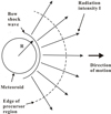 |
Fig. 6. Radiation field in the precursor region. |
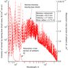 |
Fig. 7. Typical spectrum and absorption cross section of air. Abscissa is wavelength in Angstrom. The left ordinate is intensity of the normal ray leaving shock wave in the units of W/(cm2 − μm-sr), and the right ordinate is absorption cross-section in the units of cm2. |
This phenomenon will be called here, for the sake of distinction, “expansion”.
In the absence of the expansion phenomenon, radiation intensity will change as given by the equation of radiative transfer, as
 (41)
(41)
These two phenomena occur simultaneously. Therefore, the radiation intensity satisfies approximately
 (42)
(42)
Numerical integration of Eq. (42) from point 1 to point 2 results in
 (43)
(43)
where
 (44)
(44)
 (45)
(45)
Equation (43) was executed along the centerline in the precursor region. The edge of precursor region was judged to have been reached when the vacuum ultra-violet component of radiation reaches zero because of the absorption. The energy Eq. (37) was integrated in the precursor region with the radiation flux values so calculated in order to determine the thermodynamic state of the precursor region.
The enthalpy increase in the precursor region results in the increase in enthalpy behind the bow shock wave. Referring to Fig. 8, conservation of mass, momentum, and energy exists between the ambient air, Condition 1, and behind the bow shock wave, Condition 2. For the meteoroid case, some terms become negligibly small, and so
 (46)
(46)
 (47)
(47)
 (48)
(48)
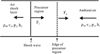 |
Fig. 8. Flow variables and direction of radiation in one-dimension around the shock wave and precursor region. In enforcing energy conservation across the shock wave, energy loss by radiative flux Fs must be accounted for. |
Iteration was carried out to determine the enthalpy behind the bow shock wave, h2, satisfying Eqs. (46)–(48). Five iterations were necessary to obtain the h2 value to within 1% error. Within the range of calculation performed in the present work, the first term in the right-hand side of Eq. (48) varied from zero to about 30% of the total of the right-hand side. This means that the loss of energy by radiation lowers the enthalpy in the shock layer, by nearly 30% for large meteoroids. The precursor region is in turn heated. At immediately ahead of the shock wave, temperature can exceed 10 000 K for large meteoroids, producing fully dissociated and partially ionized nitrogen and oxygen species. Temperature decreases gradually with distance and over many meters of this precursor region. Between the edge of the precursor region and the ground observer, the atmosphere is partly blocking through absorption and scattering. Their characteristics are well known, and will not be elaborated on here.
The precursor region will have varied and complicated influence on the spectrum observed on the ground. For instance, for a large meteoroid flying fast (for instance above 20 km s−1), the precursor region adjacent to the shock wave will contain a substantial number density of the first excited state 3s (of two spin states). Most prominent visible lines of N and O terminate at the 3s states. These lines emanating from the shock wave can be absorbed in the precursor region by the far wings of the lines. Intensity of these lines is brought down slowly as temperature falls slowly along the ray. When such a large meteoroid is flying at a slower velocity (for example 20 km s−1), the 3s states will not be excited in the precursor region, and so the visible lines of N and O will survive the precursor region and reach the ground.
At least a total of 130 iterations were made to calculate a converged solution per each value of h2. For 130 iterations, approximately 60 min was required per one value of h2 on a personal computer. Of this, 20 min was expended in generating the absorption coefficient tables and 40 min for calculating the flow and radiation fields. In the second iteration and on, the absorption coefficient tables were not calculated, and so only 40 min was required. In order to carry out five iterations over h2, therefore, 60 + 4 × 40 = 220 min were required.
3. General features of the solutions
The convergene pattern of the present approach was shown by Park (2014), and will not be given here. Spectrally the best known large meteoroid is the Benesov meteoroid. The meteoroid is believed to have fallen in 1991, and was recovered in 2011 (Spurny et al. 2014). Its mass is thought to be between 3000 and 4000 kg (Borovicka & Spurny 1996), and was taken to be 3500 kg in the present work. Its imagined chemical composition was previously described. The ideal tightly-packed density of this material is 3590 kg m−3. Borovicka et al. (1998) estimated the real density to be 2000 kg m−3, implying the porosity to be 44%. Assuming the meteoroid to be spherical in shape, its radius was calculated to be 0.75 m.
In Figs. 9 and 10, the variation patterns of the important quantities are shown at the altitude of 63.5 km. Other important parameters are given in Table 1. In Fig. 9, one sees that the thickness of the ablation-product vapor layer is of the same order as that of the air shock-layer (actually, the vapor layer thickness is three times the air layer thickness in the case shown). Temperature of air drops by 13% from the bow shock wave to the interface. At the interface, temperature drops 54% between the air layer to the vapor layer. The highest temperature of the vapor, at the edge, is about 40% of the highest temperature of air behind the bow shock wave.
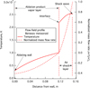 |
Fig. 9. Temperature and mass flow in shock layer and in ablation-product vapor layer as functions of distance from ablating wall for Benesov meteoroid. The abscissa is the distance from wall in meters; the left ordinate is the temperature in K; and the right ordinate is the mass flow rate normalized by its post-shock value ρv/(ρv)s. The flight altitude is 63.5 km s−1; flight velocity is 21 km s−1; nose radius is 0.75 m; and spallation factor is 1. |
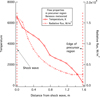 |
Fig. 10. Temperature and radiative flux in precursor region as functions of distance from the shock wave for Benesov meteoroid. The abscissa is the distance from the shock wave, the left ordinate is the temperature in K, and the right ordinate is the radiative flux in W m−2. Flight altitude, flight velocity, nose radius, and spallation factor are the same as in Fig. 9. |
Characteristics of calculated meteoroids.
In reality, of course, there will be a thin boundary layer at the interface, in which air molecules will diffuse into the vapor layer and vapor molecules will diffuse into the air layer. Within this boundary layer, velocity obeys Eq. (27) and species concentrations obey Eq. (28). Because of the analogy between diffusion and heat conduction, temperature obeys Eq. (28) also. Species concentration and temperature will have an S-shaped appearance: the two ends will asymptote to the border values shown in Fig. 9. The thickness of this boundary layer is given by Eq. (29).
That temperature drops so much between the inner-most (interface) temperature of the air layer and the outer-most (edge) temperature of the ablation-product layer, and differs so much from the determination by Park (2014), and that these two temperatures are the same. The 2014 work used Rosseland approximation, according to which radiative heat flux is a function of temperature only. In order to satisfy the condition that the radiative flux is continuous across the interface, temperature must be continuous. The present work shows that the Rosseland approximation cannot describe the two-layer situation of the meteoroid flow very well.
The thickness of the air layer is 35 mm. The thickness of the aforementioned boundary layer, Eq. (29), is calculated to be 1.0 mm. This means that the shock layer is mostly an inviscid flow. The blowing parameter, –fw, Eq. (30), is calculated to be 6.18, a value sufficiently large to qualify as massively blowing. Consequently, convective heat transfer rate is negligibly small compared with the radiative heat transfer rate.
The mean-free-path of the ambient air at 63.5 km altitude is 0.46 mm. According to Fig. 6.4 of Park (1990), equilibrium is reached behind a normal shock wave at about 7 mean-free-paths at the flight speed of 13 km s−1. If this mean-free-path value holds true for 21 km s−1, equilibrium is reached at 0.46 × 7 = 3.2 mm behind the shock wave. Because the shock layer thickness, 35 mm, is still much larger than 3.2 mm, the assumption of equilibrium flow is justified for this case.
In Fig. 11, a small segment, that is, from 5480 to 5520 A, of the true spectrum and the spectrum folded by the slit function are compared. First, one notices that the line shapes are all clean: the 400 000 wavelength points used in the present work provide sufficiently fine details of the line shapes. Though not shown, this is true of the molecular bands active in the vapor layer. Second, the folding by the Gaussian slit function averages out the line shapes in fine detail crudely.
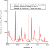 |
Fig. 11. Comparison of two intensity calculations. This is done by comparing (1) the intensity variation calculated using a fine wavelength grid and Voigt function for each line and (2) the intensity variation obtained by folding the intensity variation of (1) by a Gaussian slit function of 2.5 A half-half width, for the Benesov meteoroid. The abscissa is wavelength in Angstrom and the ordinate is the radiation intensity in W/(cm2 − μm-sr). The flight altitude, flight velocity, nose radius, and spallation factor are the same as in Fig. 9. |
In Figs. 12 and 13, the spectra of the outward-facing radiation at the interface, bow shock, end of precursor region, and ground observer are compared. The intensity of the spectrum at the ground observer station is scaled back to the bow shock wave position in order to make comparison easier. Otherwise, the ground observer spectrum would be many orders of magnitude weaker. Figure 12 shows the entire wavelength region. One sees here that vacuum ultra-violet radiation is added between the interface and shock wave by the air layer. The precursor region removes vacuum ultra-violet component more than that added by the air layer. The atmosphere removes ultra-violet component further.
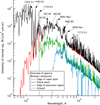 |
Fig. 12. Spectrum is shown at four sequencial positions. (1) The interface between the ablation product layer and the air shock layer, (2) the shock wave, (3) the edge of precursor region, and (4) the ground observer, over the entire spectral range, for Benesov meteoroid. The abscissa is the wavelength in Angstrom and the ordinate is the radiation intensity in W/(cm2 − μm-sr). The flight altitude, flight velocity, nose radius, and spallation factor are the same as in Fig. 9. |
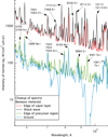 |
Fig. 13. Spectrum similar to Fig. 12, but over visible range. The abscissa is wavelength in Angstrom and the ordinate is the radiation intensity in W/(cm2 − μm-sr). |
In Fig. 13, one sees that the spectrum at the edge of the vapor layer contains atomic lines of Fe, Mg, Na, and Si. The spectrum at the shock wave shows additional lines of N and O as expected. These N and O lines terminate at the 3s (about 74 000 cm−1 for both N and O) state as mentioned, except the 7001−7002 lines of O which terminate at 3p (about 89 000 cm−1). At the edge of the precursor region, all N and O lines terminating in 3s disappear, leaving only the lines terminating in 3p; the concentration of the 3p state is insufficient in the precursor region to be absorbant. Thus the 7001−7002 O line and the lines of metals Fe, Mg, Na, and Si remain at the edge of the precursor region.
The continuum level at the edge of the precursor region is an order of magnitude lower than that at the shock wave, because of the absorption by the N and O continua in the precursor region. In the spectrum to be seen by the ground observer, the radiation at around 9500 A is depleted by the water vapor absorption in the atmosphere.
In Figs. 14 and 15, Boltzmann plots are shown for the Benesov meteoroid. The plots are calculated with Mg and Fe lines. Because the air layer is the outside layer, one would have thought that Boltzmann plot should be made with N and O lines. However, as mentioned, they are absorbed in the precursor region and are not seen by the ground observer. The first impression given by the Boltzmann plots is that the scatter is quite large. If one excuses this large scatter, the Boltzmann temperature by Mg is 12576 K and that by Fe is 10230 K. These temperatures are closest to the calculated temperature at the edge of the vapor layer, which is 10 040 K. This seems reasonable: the radiation from air is all absorbed in the precursor region.
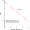 |
Fig. 14. Boltzmann plot of Benesov meteoroid spectrum using Mg I lines. The abscissa is the energy level of the upper state in cm−1 and ordinate is I/(gA) where I is the intensity in W/(cm2 − μm-sr), g is the upper state multiplicity, and A is the transition probability of the upper state in s−1. The flight altitude, flight velocity, nose radius, and spallation factor are the same as in Fig. 9. |
 |
Fig. 15. Boltzmann plot of Benesov meteoroid spectrum using Fe I lines. The abscissa is the energy level of the upper state in cm−1 and ordinate is I/(gA) where I is the intensity in W/(cm2 − μm-sr), g is the upper state multiplicity, and A is the transition probability of the upper state in s−1. The flight altitude, flight velocity, nose radius, and spallation factor are the same as in Fig. 9. |
Of particular note here is that the observed Boltzmann temperature for this case is only about 5000 K (Borovicka & Spurny 1996). Though not shown, this relatively large error in Boltzmann temperature between the observed and the presently calculated is systematic: it appears in all other cases. More work is needed here.
4. Two large meteoroids
4.1. Radiation intensity for Benesov
Calculated spectra are compared with the observations for the Benesov meteoroid in Fig. 16 for 63.5 km altitude and Fig. 17 for 40 km altitude. For the 63.5 km altitude case, the nose radius was taken to be 0.75 m, meaning the radius at the time of Earth entry. For the 40 km case, the nose radius was assumed to be 0.1071 m, meaning 1/7 of 0.75 m. For the nose radius to become 1/7 of the original, the meteoroid must be fragmented into 73 = 343 equal pieces on the average. It is tacitly assumed here that the total volume is conserved in the breakup process.
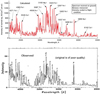 |
Fig. 16. Comparison is made between calculated and observed spectrum for Benesov meteoroid flying at the altitude of 63.5 km. Abscissa is wavelength in Angstrom. The ordinate in the top panel is the intensity in W/(cm2 − μm-sr); the ordinate in the bottom panel is intensity in arbitrary units. Flight altitude, velocity, nose radius, and spallation factor are the same as in Fig. 9. This case is favorable for calculation. |
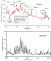 |
Fig. 17. Comparison is made between calculated and observed spectra for the Benesov meteoroid. The abscissa is wavelength in Angstrom. The ordinate in the upper panel is the intensity in W/(cm2 − μm-sr). The calculated peak intensity is approximately 10 times the observed value. Flight altitude is 40 km, flight velocity is 20.5 km s−1, nose radius is 0.1071 m, and spallation factor is 1. |
In the spectra observed and calculated in Figs. 16 and 17, strongest radiation emanates from a cluster of lines from about 4800 A to about 5500 A, with a peak at around 5200 A. 5183 Mg I is at the peak. But most of the lines in the cluster are Fe I lines. As will be seen later, this feature exists in most spectra. The first impression of Figs. 16 and 17 is that agreement is not so bad between the calculated and observed spectra, considering the fact that chemical composition of the meteoroid is assumed arbitrarily. It seems that, by tuning the chemical composition, a closer agreement could be possible. But such a tuning is outside the scope of the present work, and is left for the future. As Fig. 17 shows, the calculated intensity is approximately ten times that of the observed spectrum for the Benesov meteoroid flying at altitude of 40 km, velocity of 20.5 km s−1, nose radius of 0.1071 m, and spallation factor of 1.
It is interesting that the apparent line-widths in the calculated spectra are different between Figs. 16 and 17. In Fig. 16, the calculated line-widths are seemingly the same as the observed line-widths, while in Fig. 17, the calculated line-widths seem noticeably larger than those observed. In close examination of Fig. 17, however, one finds that the calculated weak lines are no broader than the observed weak lines. The broad calculated lines in Fig. 17 appear broad because of the over-estimated Stark widths. Overestimation of the Stark width will show its effect at high density regime of 40 km altitude. The assumed Gaussian instrument-width values are the same between Figs. 16 and 17. The Stark width is seemingly dominant over instrument width in the environment of Fig. 17.
The highest pressure on a meteoroid is at the forward stagnation point. As mentioned in 2.1, this high pressure penetrates through the porous body. A relatively long time, called incubation time by Park & Brown (2012), is required for the pressure to fill the porous body. When the body is filled with the high pressure, the meteoroid explodes. Of course, the internal pressure must be higher than the structural strength of the meteoroid, but this condition is believed to be met easily because the meteoroid is structirally quite weak. Baldwin and Sheaffer thought that on average one meteoroid splits into eight fragments (Baldwin & Sheaffer 1971). This is a reasonable statement: one can see in the photographs of Chelyabinsk meteor that it produced seven large fragments. The split fragments undergo the same fragmentation process again and again, begetting ever smaller offspring fragments. This is the process nicknamed the Medusa’s head process (Park & Brown 2012). The experiment conducted in a ballistic range (Park & Brown 2012) shows that, at least in some cases, this process converts bulk material into fine powder.
The high internal pressure pushes the fragments outward at the time of explosion. As a result, the fragments gain velocity in the outward direction during the explosion process. The theoretical model on this process correctly describes the observed outward velocity (Park & Brown 2012). This outward velocity separates the fragments. After the first-generation explosion, therefore, the fragments are some distance apart; a far distance compared with their sizes. However, after the second-generation and further explosions, some fragments are close together because some fragments move inward. As the generational explosion continues, the central core region of the cloud becomes densely crowded with with fragments. This situation is seen in Fig. 2d of Park & Brown (2012).
The Benesov meteoroid is believed to have started the breakup process when the stagnation pressure exceeded about 50 kPa (Borovicka 2016). At the 63.5 km altitude referred to in Fig. 16, the stagnation pressure is about 80 kPa: the breakup process has just begun. The radiation pattern changes with the fragmentation process, as shown schematically in Figs. 18a–c. When a meteoroid is not split, naturally radiation occurs in its shock layer, as shown in Fig. 18a. After first or second generation splitting, the fragments are far enough apart from each other and so radiation emanates only from each generations’s shock layers. The total radiation intensity observed by the ground observer will be roughly equal to the radiation intensity from one shock layer times the number of fragments.
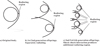 |
Fig. 18. Radiation pattern varies with fragmentation as shown schematically here. |
After several generations of splitting, some fragments are positioned so close to each other that their shock waves interact to form what is known in fluid mechanics as shock-shock interaction phenomenon, or more likely a Mach interaction which involves temporal variation and produces much higher temperatures. When this interaction is strong, the flow becomes locally subsonic as shown schematically in Fig. 18c, and, as a consequence, radiates, as shown in the theoretical calculation of Prabhu et al. (2015). This secondary radiation may become collectively stronger than the primary radiation from the shock layers depending on the situation.
By the time Benesov meteoroid reached the altitude of 40 km, it must have undergone several generations of fragmentation. That the calculation made in Fig. 17 assumes nose radius 1/7 of the original is well within the realm of possibilities. It is to be noted that (Borovicka et al. 1998) assumed that the Benesov meteoroid was in ten fragments at 40 km.
In Figs. 19 and 20, two other cases are shown in which the calculated and observed do not agree. In Fig. 19, at the altitude of 78 km, the meteoroid is warming up and vaporization of the wall has barely begun. Therefore, only the strongest spectral lines, such as 5890 Na I, 5183 Mg I, and 5267 Fe I, are visible. In contrast, in calculating the spectrum, the wall is assumed to be heated to its steady-state; vaporization and radiation emission are in steady-state. Full range of lines from Na, Mg, and Fe, led by those in the observed spectrum, are visible. As with Figs. 16 and 17, radiation is concentrated at around 5200 A, and 5183 Mg I is at the peak in the calculated spectrum. Most of the lines are Fe I lines.
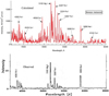 |
Fig. 19. Comparison between calculated and observed spectra for the Benesov meteoroid. The abscissa is wavelength in Angstrom. The ordinate in the top panel is the intensity in W/(cm2 − μm-sr). The ordinate in the bottom panel is intensity in arbitrary units. The flight altitude = 78 km, velocity = 21 km s−1, nose radius = 0.75 m, and spallation factor = 1. This case is unfavorable for calculation. |
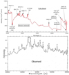 |
Fig. 20. Comparison between calculated and observed spectra for the Benesov meteoroid at altitude of 24 km. The abscissa is wavelength in Angstrom and the ordinate is the intensity in W/(cm2 − μm-sr). The flight altitude is 24 km, velocity is 14.4 km s−1, nose radius is 0.02 m, and spallation factor is 2. This case is unfavorable for calculation. |
The present theoretical calculation is not expected to match the observation for the 24 km case in Fig. 20. By the time the meteoroid reached the altitude of 24.3 km, the meteoroid mass had undergone a series of unequal splitting processes and thereby produced several sub-groups of different sizes. The upper and lower figures in Fig. 20 are very different and only a few common spectral lines can be found. There is a large difference in the bound-free continuum of air species, which is affected in turn by the precursor phenomenon. Explaining the difference between the calculated and observed spectra would seem impossible. Still there is a redeeming quality in the calculation: the ratio of calculated intensities between lines and continuum agree roughly with the observations.
4.2. Benesov light curve
In Figs. 21 and 22, the light curve for Benesov meteoroid is shown and is compared with the calculations. The brightness magnitude M̃ was determined in the present work as follows: the Sun irradiates Earth’s surface with an irradiance of 1364.9 W m−2, and this is defined to be a magnitude of −26.74. The meteoroid radiates from the edge of the precursor region with a flux of Fp W m−2. Multiplying by the radiating area πR2, one obtains radiating source power FpπR2 in Watts. If there is more than one meteoroids (radiating in the same way), FpπR2 is multiplied by the number of those meteoroids. The meteoroid is at an altitude of S. The irradiance on the ground is FpπR2 divided by the half-global area 2πS2. Therefore, the irradiance produced by the meteoroid on the ground is FpπR2/(2πS2) W m−2. This quantity was divided by 1364.9 W m−2. The resulting quantity was expressed in magnitude, where magnitude 1 means a ratio of 1000.2 = 2.511886. When this quantity was added to −26.74, the brightness magnitude M̃ of the meteoroid was obtained.
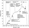 |
Fig. 21. Overview of light curve for the Benesov meteoroid and calculated values of brightness magnitude. The abscissa is the altitude in km and the ordinate is the brightness magnitude. |
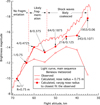 |
Fig. 22. Main sequence of the Benesov meteoroid light curve and calculated values of brightness magnitude. The abscissa is the altitude in km and the ordinate is the brightness magnitude. |
In Fig. 21, an overview is given. In the earliest time period, the meteoroid is warming up from the cold initial temperature to the hot steady-state temperature. In this period, ablation rate is either zero or at best smaller than the value obtained by the present steady-state assumption. In Fig. 19, comparison was made between the spectrum calculated by the present method with the observed spectrum at the altitude of 78 km. Therein, the calculated spectrum showed stronger radiation than what was observed. In Fig. 21, the brightness values corresponding to these two calculations are shown: the open circle at magnitude of −11.1 is the value calculated by the steady-state assumption, which is much higher than the observed value represented by the solid curve, itself about −6.4. The present calculation assuming zero ablation (spallation factor = 0) shown by the solid circle agrees with the observed value.
The warming-up period is followed by what is named in the present work the main sequence period. In this period, steady-state ablation is maintained and radiation pattern is one of the three shown in Figs. 18a–c. The main sequence period is still divided into two periods. In the first period, the fragments are separated far enough and there are no shock-shock interactions. The radiation pattern is that shown in Fig. 18a or b. In the second period, shock-shock interaction produces additional radiation, as shown in Fig. 17c.
In Fig. 22, a detailed comparison is made between the calculated and observed brightness magnitudes in the main sequence period. To each calculated point, either solid or open circles, two numbers were attached. The first number, n, is the number of fragments, and the second number, R, is the nose radius. The n and R were determined assuming the total volume is conserved: the ablation effect will be small in the present thought process. There were two sets of calculated brightness magnitude values. The closed symbols show the calculations made to produce the brightness magnitude values closest to the observed values. This was done by varying the radius of individual meteoroid fragments R and the n number matching the R. The brightness from one fragment in Watts was multiplied by n to obtain the total brightness in Watts before being converted into magnitude M̃. As seen, in the first period when radiation is either Fig. 18a or b type, there is a good agreement between the calculated and the observed. In the second period, calculated values fall short of observations because the radiation caused by shock-shock interaction is not accounted for. The open circles show the brightness magnitudes obtained by the fixed nose radius of R = 0.75 m. Needless to say, this no-fragmentation option underestimates brightness severely. The number of fragments deduced from Fig. 22 is quite large: many generations of fragmentation is occurring for Benesov meteoroid, true to the name of Medusa’s head.
The main sequence period is followed by a pulverized period, a period in which the fragments are very small and very numerous. Remarkably, the present calculation reproduces the observed brightness magnitude as seen in Fig. 21. The calculated spectrum, shown in Fig. 20 does not resemble the observed spectrum much, though.
4.3. Sumava meteoroid
Following Borovicka & Spurny (1996), Sumava meteoroid was assumed to have a mass of 5000 kg and average density of 100 kg m−3. This results in a radius of approximately 2 m. The low value of density suggests that the meteoroid was more likely a comet (Nemtchinov et al. 1999). The composition of cometary meteoroids most likely corresponds to that of a carbonaceous chondrite. Therefore, the chemical composition assumed for the Benesov meteoroid should be suitable for the Sumava meteoroid also.
In Fig. 23, calculated brightness magnitude values, shown as solid circles, are compared with the observed light curves values shown as a solid curve. The two numbers associated with each solid circles are the number of fragments and nose radius, as were in Fig. 22. The calculated values agree with the observed values.
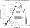 |
Fig. 23. Light curve for Sumava meteoroid. The abscissa is the altitude in km and the ordinate is the brightness magnitude. |
In Fig. 24, calculated spectra are shown for two altitude points in Fig. 23. There are no observed spectra to compare. At least theoretically, line radiation is concentrated at around 5200 A, and the 5183 Mg I line is at its peak, as was the case for the Benesov meteoroid. But, unlike Benesov meteoroid, Sumava’s spectra contain strong continua. This is probably because absorption is weak in the precursor region. This is in turn because the density of the ambient air is low, meaning altitude is high, for the Sumava meteoroid.
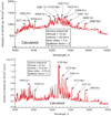 |
Fig. 24. Spectra are calculated for Sumava meteoroid. The abscissa is wavelength in Angstrom and ordinate is intensity of normal ray in W/(cm2 − μm-sr). |
5. Other aspects
5.1. Effect of chemical composition on spectrum
A question arises as to how much the chemical composition of a meteoroid will affect the spectrum and the associated brightness magnitude. In order to answer this question, calculation was made of the spectrum and brightness magnitude at 63.5 km altitude, 21 km s−1 velocity, and 0.75 m nose radius for some of the known meteorites. Chemical compositions of these meteorites are presented in Table C.1. In Figs. C.1–C.4, the calculated spectra of these meteoroids are shown. Table 1 lists other characteristics. There appear to be substantial differences among their spectra and brightness magnitudes. These results suggest that it may be possible to deduce the chemical compositions from the spectra and brightness magnitudes, by using the computer code presented below.
5.2. Ablation rate and luminous efficiency
Luminous efficiency is defined as Pecina & Kolten (2009)
 (49)
(49)
Radiation power emitted is, however, determined by the ground observer from a black body type radiometer or a spectrograph, at the vertical bar position at far right in Fig. 1b. The power lost in ablation is the enthalpy of the flow entering the bow shock wave multiplied by the ablation rate. For both quantities, areal integration is required. As mentioned earlier, by assuming the angular (Θ) distribution to be a cosine function, the areal integration becomes simply a multiplication of πR2;
 (50)
(50)
The luminous efficiency values so determined are listed in Table 1. The calculated values are typically a few percent. In the past, luminous efficiency values were assumed to have a value of a few percent, without a firm scientific justification. It seems that such assumption was justified. By using the present computer code, this quantity is calculated rationally.
5.3. Small meteoroids
A question arises as to what will happen if the present method is applied to a small meteoroid. To answer such a question, calculations were performed for a yet unanalyzed small meteoroid tentatively identified as 20151230–222303 (Koukal 2016). The mass and entry velocity of this meteoroid are believed to be 0.200 kg and 15 km s−1, respectively (Koukal 2016). One spectrum was taken, but the altitude where it was taken is not given Koukal (2016). In the present work, calculations were done assuming the average density to be 2000 km s−3, leading to the nose radius of approximately 0.03 m. The chemical composition was assumed to be a typical H-chondrite as shown in Table C.1. The flight altitude was taken arbitrarily to be 63.5 km. The calculated spectrum is compared with the observed spectrum in Fig. 24. Other characteristics are listed in Table 1. The calculated brightness magnitude is −2.75; the observed value was −3.65.
In Fig. 24, one sees that the present calculation cannot be applied to small meteoroids. As mentioned earlier (see Sect. 3), the distance to reach ionization equilibrium is 3.2 mm at the altitude of 63.5 km. Shock stand-off distance for Koukal2303 meteoroid is 1.1 mm. The shock layer flow is in a thermo-chemical nonequilibrium state: degree of ionizaton is lower than the equilibrium value. The low degree of ionization will cause lowered continuum in the spectrum. Nonequilibrium phenomenon must be accounted for to calculate the radiation phenomena for small meteoroids.
6. Discussion
The computer code developed in the present work, meteor-spect.f90, when combined with a fragmentation theory, seemingly can reproduce the observed light curves fairly closely and spectra approximately for large meteoroids. In the future, when a large meteoroid enters the atmosphere and if a light curve or spectrum is obtained, meteor-spect.f90 code should be able to help in analyzing the observed data.
The present work uncovers the reason for one peculiar phenomenon hitherto unexplained. When a Boltzmann plot is made with an obtained spectrum, it is possible mostly with the ablation-product vapor species. The Boltzmann temperature obtained is close to the temperature of the vapor at the edge of the vapor layer. This vapor temperature is about half or less of the shock layer temperature; there is a discontinuity in temperature across the air-to-vapor interface. The hot air layer generates strong radiation from nitrogen and oxygen species, but that radiation is absorbed in the precursor region.
The most important improvement needed on the meteor-spect.f90 code will be on Stark line-widths. It will be a quite tedious work to calculate Stark widths. As mentioned earlier, the present work does not account for the lowering of ionization potential by electrons and by heavy particles. Improvement is welcome here also.
At this point, one may contemplate what lies ahead along the present path of formulating the radiation problem for meteoroids. Beyond the Stark width problem cited above, one will have to face the general problems for small meteoroids, namely the problem of thermo-chemical non-equilibrium and viscous mixing phenomena. Formalisms for these two problems are no different from the problems solved in the past for flight velocities below 13 km s−1. Difficulties arise because there are no experimental data on reaction rates or momentum- or energy-transfer cross-sections for higher flight velocities. One will have to generate the necessary parameters entirely by theory from the theoretically-determined potential energy surfaces. Perhaps the procedure will be easier because the emphasis will be on the high-energy portion of the potential energy surfaces which will be beyond the usually-troublesome energy-minimum or energy-maximum points and surfaces.
But one distinctly different problem the small meteoroids will bring is the influence of the precursor phenomenon on the starting conditions of the shock wave. The precursor phenomena will bring the air molecules entering the shock wave in forms that are already partly dissociated, ionized, and rotationally, vibrationally, and electronically excited, at least partially. The level of these excitations will affect the relaxation processes behind the shock wave.
One may erroneously hope that the direct-simulation Monte-Carlo (DSMC) approach will solve all these problems. It does not. DSMC techniques need all the physical parameters the continuum methods need, and yet others more related to modeling the large number events into small number events. The present author encourages future scientists challenging these problems.
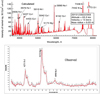 |
Fig. 25. Comparison is made between the observed and calculated spectra for 20151230–222303 meteoroid. Abscissa is wavelength in Angstrom and ordinate is intensity of normal ray in W/(cm2 − μm-sr). |
7. Conclusions
The radiation phenomena occurring during the atmospheric entry flights of meteoroids are investigated for large meteoroids assuming thermochemical equilibrium and inviscid flow.
-
The investigation finds that the ablation-product vapor forms a thick layer inside the shock layer formed by air. There is a large jump in temperature at the interface between the two layers, and the temperature of the vapor at the interface is less than half of the temperature behind the shock wave.
-
The Boltzmann plots made with the lines of the vapor species tend to be indicative of the temperature of the vapor at the interface. The precursor region in front of the shock wave absorbs line radiation from nitrogen and oxygen emitted by the hot shock layer, and therefore these lines cannot be used for the Boltzmann plot.
-
For the Benesov meteoroid, the spectra calculated in this work are fairly similar to the observed spectra. For both Benesov meteoroid and Sumava meteoroid, the brightness magnitudes calculated by the present method are in agreement with the observation, when fragmentation is taken into account. Luminous efficiency values calculated as a byproduct roughly match the values assumed and used in the past.
SPRADIAN07 is available unlimitedly by contacting Dr. Seong-Yoon Hyun, This email address is being protected from spambots. You need JavaScript enabled to view it.
References
- Arnold, J. O., Cooper, D. M., & Park, C. 1979, American Institute of Aeronautics and Astronautics, Washington, DC, AIAA Paper 79–1082 [Google Scholar]
- Baldwin, B., & Sheaffer, Y. 1971, J. Geophys. Res., 76, 4653 [NASA ADS] [CrossRef] [Google Scholar]
- Bear, J. 1972, Dynamics of Fluids in Porous Media (New York: Dover) [Google Scholar]
- Borovicka, J. 2016, IAU Symp., 318, 80 [NASA ADS] [Google Scholar]
- Borovicka, J., & Spurny, P. 1996, Icarus, 121, 484 [NASA ADS] [CrossRef] [Google Scholar]
- Borovicka, J., Popova, O. P., Golub, A. P., Kosarev, I. B., & Nemtchinov, I. V. 1998, A&A, 337, 591 [NASA ADS] [Google Scholar]
- Ceplecha, Z., & McCrosky, R. E. 1976, J. Geophys. Res., 81, 6258 [NASA ADS] [Google Scholar]
- Chase, Jr., M. W. 1998, J. Phys. Chem. Ref. Data Monograph No. 9, 1963 [Google Scholar]
- Chyba, C. F. 1997, Nature, 389, 234 [NASA ADS] [CrossRef] [Google Scholar]
- Davies, C. B., & Park, C. 1983, in Progress in Astronautics and Aeronautics, eds. P. E. Bauer, & H. E. Collicott, 85, 372 [Google Scholar]
- Fujita, K., & Abe, T. 1997, Institute of Space and Aeronautical Sciences, Japan Aerospace Exploration Agency, Tokyo, Japan, ISAS Report 669 [Google Scholar]
- Glavin, D. P., Elsila, J. E., Burton, A. S., et al. 2012, Meteorit. Planet. Sci., 47, 1347 [NASA ADS] [CrossRef] [Google Scholar]
- Hyun, S. Y. 2009, PhD Thesis Dept. of Aerospace Engineering, Korea Advanced Institute of Science and Technology, Daejeon, Korea [Google Scholar]
- Jarosewich, E. 1990, Meteoritics, 75, 323 [NASA ADS] [CrossRef] [Google Scholar]
- Koukal, J. 2016, Meteor News, Nov. 20 [Google Scholar]
- Kovacs, I. 1969, Rotational Structure in the Spectra of Diatomic Molecules, Adam Hilger, London [Google Scholar]
- Libby, P. A. 1970, AIAA J., 8, 2095 [NASA ADS] [CrossRef] [Google Scholar]
- Nemtchinov, I. V., Kumicheva, M. Yu., Shuvalov, V. V., et al. 1999, in Proc. IAU Coll., eds. J. Svoren, E. M. Pittich, & H. Rickman, 173, 51 [NASA ADS] [Google Scholar]
- Omura, M., & Presley, A. 1969, AIAA J., 7, 2363 [NASA ADS] [CrossRef] [Google Scholar]
- Park, C. 1990, Nonequilibrium Hypersonic Aerothermodynamics (New York: John Wiley and Sons) [Google Scholar]
- Park, C. 1999, J. Thermophys. Heat Transf., 13, 441 [CrossRef] [Google Scholar]
- Park, C. 2004, J. Thermophys. Heat Transf., 18, 349 [CrossRef] [Google Scholar]
- Park, C. 2009, J. Thermophys. Heat Transf., 23, 417 [CrossRef] [Google Scholar]
- Park, C. 2013, J. Quant. Spectrosc. Radiat. Transf., 127, 158 [Google Scholar]
- Park, C. 2014, J. Thermophys. Heat Transf., 28, 598 [NASA ADS] [CrossRef] [Google Scholar]
- Park, C. 2015, J. Quant. Spectr. Rad. Transf., 154, 44 [NASA ADS] [CrossRef] [Google Scholar]
- Park, C., & Ahn, H. K. 1998, J. Thermophys. Heat Transf., 13, 33 [CrossRef] [Google Scholar]
- Park, C., & Brown, J. D. 2012, AJ, 144, 1 [CrossRef] [Google Scholar]
- Park, C., Raiche, G. A., & Driver, D. M. 2004, J. Thermophys. Heat Transf., 18, 519 [CrossRef] [Google Scholar]
- Peach, G. 1978, Mem. Astron. Soc., 73, 1 [NASA ADS] [Google Scholar]
- Pecina, P., & Kolten, P. 2009, A&A, 499, 313 [NASA ADS] [CrossRef] [EDP Sciences] [Google Scholar]
- Prabhu, D. K., Agrawal, P., Allen, Jr., G. A., et al. 2015, 4th IAA Planetary Defense Conference, Rome, Italy, IAA-PDC-15-OX-XX [Google Scholar]
- Spurny, P., Haloda, J., Borovicka, J., Shrbeny, L., & Hlodova, P. 2014, A&A, 570, A39 [NASA ADS] [CrossRef] [EDP Sciences] [Google Scholar]
- Stackpoole, M., Kao, D., Qu, V., & Gonzales, G. 2013, Post-Flight Evaluation of PICA and PICA-X – Comparisons of the Stardust SRC and Space-X Dragon 1 Forebody Heatshield Materials, 2013, ARC-E-DAA-TN 9994 [Google Scholar]
- Tran, H. K., Johnson, C. E., Rasky, D. J., et al. 1997, Phenolic Impregnated Carbon Ablators (PICA) as Thermal Protection Systems for Discovery Missions, NASA TM 110440 [Google Scholar]
- Whiting, E. E., Arnold, J. O., & Lyle, G. C. 1969, NASA TN D-5088 [Google Scholar]
- Winter, M. W., & Trumble, K. A. 2011, J. Spacecr. Rocket., 48, 59 [NASA ADS] [CrossRef] [Google Scholar]
- Winter, M. W., McDaniel, R. D., Chen, Y. K., et al. 2012, American Institute of Aeronautics and Astronautics, Washington, DC, AIAA Paper 2012–1296 [Google Scholar]
Appendix A: Nomenclature
1: Air shock layer.
2: Ablation product layer.
B: Planck function, W/(cm2 − μm-sr).
Bλ: Planck function value at wavelength λ.
Ep: Ionization potential.
e: Edge of ablation layer.
f: Freestream or velocity function in viscous flow, Eq. (26).
fw: Blowing parameter, Eq. (30).
 : Velocity function in inviscid flow, Eq. (15).
F: Radiative heat flux, W m−2.
g: Multiplicity.
h: Enthalpy, J kg−1.
I: Radiation intensity, W/(cm2 − μm-sr).
Iλ: Intensity at wavelength λ.
i: Inner edge of shock layer.
j: Spallation factor.
K: Permeability, m2.
Ṁ: Ablation rate per unit cross sectional area, kg/(m2-s).
M: Mass flow rate, kg s−1.
Ṁ: Mass flow rate per unit cross sectional area, kg/(m2-s).
M1: Radial flow rate in air shock layer, kg s−1.
M2: Radial flow rate in ablation product layer, kg s−1.
M̃: Brightness magnitude.
Ne: Electron density, cm−3.
n: Number of fragments.
p: Pressure, Pascal.
Q: Energy flow, W.
 : Energy flow per unit cross sectional area, W m−2.
Q1: Radial energy flow in air shock layer, W.
Q2: Radial energy flow in ablation product layer, W.
r: Radial distance from the axis of symmetry, m.
R: Nose radius, m.
S: Altitude, m.
s: Shock wave.
T: Temperature, K.
u: Velocity component tangential to wall, m s−1.
v: Velocity component normal to wall, m s−1.
V: Flight velocity, m s−1.
y: Distance normal to wall, m.
z: Species mass fraction.
α: A parameter in Stark width, Eq. (1).
β: A parameter in Stark width, Eq. (1).
Δλ: Wavelength interval, A.
ΔH: Ablation energy, J kg−1.
ϵ: Emission coefficient, W/(cm3 − μm-sr).
ϵλ: Emission coefficient at wavelength λ.
η: Normalized normal coordinate in viscous flow.
 : Normal coordinate in inviscid flow, m.
ηL: Luminous efficiency.
κ: Absorption coefficient, cm−1.
κ1: Quantity defined in Eq. (28).
κλ: Absorption coefficient at wavelength λ.
λ: Wavelength, A.
μ: Viscosity, kg/(m-s).
ρ: Density, kg m−3.
Θ: Polar angle, radian.
Superscript
′:  .
.
Subscript
e: Outer edge of ablation-product vapor layer.
f: Free-stream.
g: Ground observer.
i: Inner edge of air shock layer.
p: Precursor region.
pk: Peak.
s: Shock wave.
t: Total.
tr: True.
V: Voigt profile.
w: Wall.
λ: Wavelength.
Appendix B: Meteor-spect.f90
The computer code package developed in the present work, meteor-spect.f90, consists of (1) one Fortran F90 source code of 17196 lines named meteor-spect.f90; (2) one atomic radiation data file atom.dat, of 51687 lines; (3) one diatomic radiation data file diatom.dat, of 5736 lines; (4) one triatomic radiation data file triatom.dat, of 1284 lines; (5) one equilibrium air table with viscosity data eqtab-air-vis.dat, of 3837 lines; and (6) one run data file meteor-spect.inp, of 10717 lines. One run takes approximately 220 min on a personal computer. Of this, approximately 20 min are for generation of radiation tables, and 40 min are for the flow-field calculations. The radiation tables so generated can be used next time if the free-stream density and flight velocity are unchanged. One run produces nine output files. The entire package is open for free access and use. It should be obtained from:
The author of the meteor-spect.f90 code: Chul Park, This email address is being protected from spambots. You need JavaScript enabled to view it.
The co-owners of the code package are:
-
(1)
KAIST (Korea Advanced Institute of Science and Technology), c/o Prof. Gisu Park, This email address is being protected from spambots. You need JavaScript enabled to view it. ; and Dr. Seong-Yoon Hyun, This email address is being protected from spambots. You need JavaScript enabled to view it. , and
-
(2)
JAXA (Japan Aerospace Exploration Agency), c/o Dr. Kazuhisa Fujita, This email address is being protected from spambots. You need JavaScript enabled to view it.
Contact points are:
-
(1)
NASA Ames Research Center, c/o Dr. James O. Arnold, This email address is being protected from spambots. You need JavaScript enabled to view it. ; c/o Dr. Petrus Jenniskins, This email address is being protected from spambots. You need JavaScript enabled to view it.
-
(2)
Astronomical Institute of the Academy of Sciences, Czech Republic, c/o Dr. Jiri Borovicka, This email address is being protected from spambots. You need JavaScript enabled to view it.
-
(3)
Russian Academy of Sciences, Moscow, c/o Prof. Sergey Surzhikov, This email address is being protected from spambots. You need JavaScript enabled to view it.
Appendix C: Spectra of meteoroids of various chemical compositions
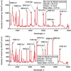 |
Fig. C.1. Spectra calculated for the San Juan de Allende and Valle de Allende meteoroids with chemical compositions given in Table C.1. |
The spectra for the Allende chondrules are devoid of iron, and so spectral lines are those of Mg, Ca, and Na. Radiation is not concentrated around 5200 A: these two meteoroids are the only exception. The radiative heat flux leaving the shock layer, Fs in Table 1, the one reaching the ground, Fg, and the meteoroid’s brightness magnitude are all also relatively small. The Clovis meteoroid contains all chemical compounds accounted for in the present model meteoroid, and so its spectrum looks similar to that of the calculated Benesov meteoroid. Most of spectral lines are those of iron. The Campo del Cielo meteoroid has iron in a markedly small quantity according to Jarosewich (1990). As a result, the spectrum consists of a small amount of iron and mostly of Mg, Ca, and Si lines. The brightness magnitude is noticeably smaller than others, and, likely as a consequence, a relatively large luminous efficiency. This spectrum serves the purpose in the present work of showing the effect of varied chemical compositions, but is not to be taken to represent the spectrum of the actual Campo del Cielo meteoroid because the bulk meteorrite contains in fact a lot of iron. MAC88105 is low on Fe and Mg but high in Ca. Its spectrum is rich with Ca lines. The brightness magnitude is relatively high. Orgueil has a chemical composition that is not much different from the present model composition, except for its high water content. The H atoms in the ionized state produce the high continuum seen in the spectrum. Woodbine is composed almost entirely of Fe. In the middle region of the spectrogram, many Fe lines are ganged up to produe a tower-like appearance. (The tower-like appearance is not due to black body saturation.) Vaca Muerta is lean on Fe. The spectra look also lean of Fe lines. The brightness magnitude is also relatively low.
Mass percentages of compounds in meteoroids; present work and meteoroids resulting in different spectrum.
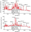 |
Fig. C.2. Spectra calculated for the Clovis and Campo del Cielo meteoroids with chemical compositions given in Table C.1. |
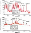 |
Fig. C.3. Spectra calculated for the MAC88105 and Orgueil meteoroids with chemical compositions given in Table C.1. |
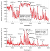 |
Fig. C.4. Spectra calculated for the Woodbine and Vaca Muerta meteoroids with chemical compositions given in Table C.1. |
All Tables
Mass percentages of compounds in meteoroids; present work and meteoroids resulting in different spectrum.
All Figures
|
Fig. 1. Acquisition process of radiation emitted by a meteoroid, shown schematically. Top panel: two-dimensional depiction of the light beam path captured by the ground observer. Bottom panel: this two-dimensional light path is replaced by a horizontal line to represent the two-dimensional affair into a one-dimensional affair. |
| In the text | |
|
Fig. 2. Overall view of ablating meteoroid. For a slightly porous meteoroid (panel a), a layer of liquid melt forms over the solid meteoroid. For a highly porous meteoroid, (panel b), a layer of densified solid forms below the liquid layer. Air molecules pass through the holes existing in the liquid layer and the densified solid layer, eventually permeating through the porous solid. |
| In the text | |
|
Fig. 3. Stagnation region flow-field of ablating meteoroid. In the frontal region of a meteoroid flying through the atmosphere, two distinct layers of gaseous state form behind the bow shock wave, one by air (shock layer) in the outer region and the other by the ablation-product (ablation layer) in the inner region. The quantities flowing axially are denoted with dots, that is, Ṁ and Q̇, and are per area per sec. The quantities flowing radially are denoted without dots, that is M and Q, and are per sec. |
| In the text | |
|
Fig. 4. Three-dimensional incompressible inviscid flow blowing normally against a flat plate. Radial distance is x, and vertical distance is y. Streamline and stagnation points are indicated. |
| In the text | |
|
Fig. 5. Profile of the 5001.86 Fe I line. Abscissa is wavelength in Angstrom and ordinate is absorption coefficient in arbitrary units. Wavelength step is 9.00 A. The wavelength mesh point closest to 5001.86 A is 5000 A. |
| In the text | |
|
Fig. 6. Radiation field in the precursor region. |
| In the text | |
|
Fig. 7. Typical spectrum and absorption cross section of air. Abscissa is wavelength in Angstrom. The left ordinate is intensity of the normal ray leaving shock wave in the units of W/(cm2 − μm-sr), and the right ordinate is absorption cross-section in the units of cm2. |
| In the text | |
|
Fig. 8. Flow variables and direction of radiation in one-dimension around the shock wave and precursor region. In enforcing energy conservation across the shock wave, energy loss by radiative flux Fs must be accounted for. |
| In the text | |
|
Fig. 9. Temperature and mass flow in shock layer and in ablation-product vapor layer as functions of distance from ablating wall for Benesov meteoroid. The abscissa is the distance from wall in meters; the left ordinate is the temperature in K; and the right ordinate is the mass flow rate normalized by its post-shock value ρv/(ρv)s. The flight altitude is 63.5 km s−1; flight velocity is 21 km s−1; nose radius is 0.75 m; and spallation factor is 1. |
| In the text | |
|
Fig. 10. Temperature and radiative flux in precursor region as functions of distance from the shock wave for Benesov meteoroid. The abscissa is the distance from the shock wave, the left ordinate is the temperature in K, and the right ordinate is the radiative flux in W m−2. Flight altitude, flight velocity, nose radius, and spallation factor are the same as in Fig. 9. |
| In the text | |
|
Fig. 11. Comparison of two intensity calculations. This is done by comparing (1) the intensity variation calculated using a fine wavelength grid and Voigt function for each line and (2) the intensity variation obtained by folding the intensity variation of (1) by a Gaussian slit function of 2.5 A half-half width, for the Benesov meteoroid. The abscissa is wavelength in Angstrom and the ordinate is the radiation intensity in W/(cm2 − μm-sr). The flight altitude, flight velocity, nose radius, and spallation factor are the same as in Fig. 9. |
| In the text | |
|
Fig. 12. Spectrum is shown at four sequencial positions. (1) The interface between the ablation product layer and the air shock layer, (2) the shock wave, (3) the edge of precursor region, and (4) the ground observer, over the entire spectral range, for Benesov meteoroid. The abscissa is the wavelength in Angstrom and the ordinate is the radiation intensity in W/(cm2 − μm-sr). The flight altitude, flight velocity, nose radius, and spallation factor are the same as in Fig. 9. |
| In the text | |
|
Fig. 13. Spectrum similar to Fig. 12, but over visible range. The abscissa is wavelength in Angstrom and the ordinate is the radiation intensity in W/(cm2 − μm-sr). |
| In the text | |
|
Fig. 14. Boltzmann plot of Benesov meteoroid spectrum using Mg I lines. The abscissa is the energy level of the upper state in cm−1 and ordinate is I/(gA) where I is the intensity in W/(cm2 − μm-sr), g is the upper state multiplicity, and A is the transition probability of the upper state in s−1. The flight altitude, flight velocity, nose radius, and spallation factor are the same as in Fig. 9. |
| In the text | |
|
Fig. 15. Boltzmann plot of Benesov meteoroid spectrum using Fe I lines. The abscissa is the energy level of the upper state in cm−1 and ordinate is I/(gA) where I is the intensity in W/(cm2 − μm-sr), g is the upper state multiplicity, and A is the transition probability of the upper state in s−1. The flight altitude, flight velocity, nose radius, and spallation factor are the same as in Fig. 9. |
| In the text | |
|
Fig. 16. Comparison is made between calculated and observed spectrum for Benesov meteoroid flying at the altitude of 63.5 km. Abscissa is wavelength in Angstrom. The ordinate in the top panel is the intensity in W/(cm2 − μm-sr); the ordinate in the bottom panel is intensity in arbitrary units. Flight altitude, velocity, nose radius, and spallation factor are the same as in Fig. 9. This case is favorable for calculation. |
| In the text | |
|
Fig. 17. Comparison is made between calculated and observed spectra for the Benesov meteoroid. The abscissa is wavelength in Angstrom. The ordinate in the upper panel is the intensity in W/(cm2 − μm-sr). The calculated peak intensity is approximately 10 times the observed value. Flight altitude is 40 km, flight velocity is 20.5 km s−1, nose radius is 0.1071 m, and spallation factor is 1. |
| In the text | |
|
Fig. 18. Radiation pattern varies with fragmentation as shown schematically here. |
| In the text | |
|
Fig. 19. Comparison between calculated and observed spectra for the Benesov meteoroid. The abscissa is wavelength in Angstrom. The ordinate in the top panel is the intensity in W/(cm2 − μm-sr). The ordinate in the bottom panel is intensity in arbitrary units. The flight altitude = 78 km, velocity = 21 km s−1, nose radius = 0.75 m, and spallation factor = 1. This case is unfavorable for calculation. |
| In the text | |
|
Fig. 20. Comparison between calculated and observed spectra for the Benesov meteoroid at altitude of 24 km. The abscissa is wavelength in Angstrom and the ordinate is the intensity in W/(cm2 − μm-sr). The flight altitude is 24 km, velocity is 14.4 km s−1, nose radius is 0.02 m, and spallation factor is 2. This case is unfavorable for calculation. |
| In the text | |
|
Fig. 21. Overview of light curve for the Benesov meteoroid and calculated values of brightness magnitude. The abscissa is the altitude in km and the ordinate is the brightness magnitude. |
| In the text | |
|
Fig. 22. Main sequence of the Benesov meteoroid light curve and calculated values of brightness magnitude. The abscissa is the altitude in km and the ordinate is the brightness magnitude. |
| In the text | |
|
Fig. 23. Light curve for Sumava meteoroid. The abscissa is the altitude in km and the ordinate is the brightness magnitude. |
| In the text | |
|
Fig. 24. Spectra are calculated for Sumava meteoroid. The abscissa is wavelength in Angstrom and ordinate is intensity of normal ray in W/(cm2 − μm-sr). |
| In the text | |
|
Fig. 25. Comparison is made between the observed and calculated spectra for 20151230–222303 meteoroid. Abscissa is wavelength in Angstrom and ordinate is intensity of normal ray in W/(cm2 − μm-sr). |
| In the text | |
|
Fig. C.1. Spectra calculated for the San Juan de Allende and Valle de Allende meteoroids with chemical compositions given in Table C.1. |
| In the text | |
|
Fig. C.2. Spectra calculated for the Clovis and Campo del Cielo meteoroids with chemical compositions given in Table C.1. |
| In the text | |
|
Fig. C.3. Spectra calculated for the MAC88105 and Orgueil meteoroids with chemical compositions given in Table C.1. |
| In the text | |
|
Fig. C.4. Spectra calculated for the Woodbine and Vaca Muerta meteoroids with chemical compositions given in Table C.1. |
| In the text | |
Current usage metrics show cumulative count of Article Views (full-text article views including HTML views, PDF and ePub downloads, according to the available data) and Abstracts Views on Vision4Press platform.
Data correspond to usage on the plateform after 2015. The current usage metrics is available 48-96 hours after online publication and is updated daily on week days.
Initial download of the metrics may take a while.