| Issue |
A&A
Volume 631, November 2019
|
|
|---|---|---|
| Article Number | A54 | |
| Number of page(s) | 8 | |
| Section | Atomic, molecular, and nuclear data | |
| DOI | https://doi.org/10.1051/0004-6361/201935789 | |
| Published online | 18 October 2019 | |
Synthesizing carbon nanotubes in space
1
School of Engineering Sciences in Chemistry, Biotechnology and Health, Department of Theoretical Chemistry & Biology, Royal Institute of Technology, 10691 Stockholm, Sweden
e-mail: This email address is being protected from spambots. You need JavaScript enabled to view it.
2
Department of Physics and Astronomy, University of Missouri, Columbia, MO 65211, USA
e-mail: This email address is being protected from spambots. You need JavaScript enabled to view it.
Received:
26
April
2019
Accepted:
19
September
2019
Abstract
Context. As the fourth most abundant element in the universe, carbon (C) is widespread in the interstellar medium (ISM) in various allotropic forms (e.g. fullerenes have been identified unambiguously in many astronomical environments, the presence of polycyclic aromatic hydrocarbon molecules in space has been commonly acknowledged, and presolar graphite, as well as nanodiamonds, have been identified in meteorites). As stable allotropes of these species, whether carbon nanotubes (CNTs) and their hydrogenated counterparts are also present in the ISM or not is unknown.
Aims. The aim of the present works is to explore the possible routes for the formation of CNTs in the ISM and calculate their fingerprint vibrational spectral features in the infrared (IR).
Methods. We studied the hydrogen-abstraction and acetylene-addition (HACA) mechanism and investigated the synthesis of nanotubes using density functional theory (DFT). The IR vibrational spectra of CNTs and hydrogenated nanotubes (HNTs), as well as their cations, were obtained with DFT.
Results. We find that CNTs could be synthesized in space through a feasible formation pathway. CNTs and cationic CNTs, as well as their hydrogenated counterparts, exhibit intense vibrational transitions in the IR. Their possible presence in the ISM could be investigated by comparing the calculated vibrational spectra with astronomical observations made by the Infrared Space Observatory, Spitzer Space Telescope, and particularly the upcoming James Webb Space Telescope.
Key words: astrochemistry / molecular data / molecular processes / ISM: lines and bands / infrared: ISM / ISM: molecules
© ESO 2019
1. Introduction
Carbon (C) is the fourth (by mass) most abundant element in the universe. Due to its unique electronic structure, three types of chemical bonds, sp1, sp2, and sp3 hybridizations, can be formed. Such a property facilitates C in building various multi-atomic structures with different molecular configurations, including amorphous carbon, diamonds, graphite, graphene, fullerenes, carbon buckyonions, carbon nanotubes, and planar polycyclic aromatic hydrocarbon (PAH) molecules (Henning & Salama 1998).
Many of these carbonaceous compounds have been detected in the interstellar medium (ISM) either through their fingerprint spectral features in the infrared (IR), or through isotope analysis of primitive meteorites. The latter leads to the identification of presolar nanodiamonds and graphite of interstellar origin (Li & Mann 2012). Solid hydrogenated amorphous carbon reveals their presence in the low-density ISM through the 3.4 μm aliphatic C–H absorption feature (Pendleton & Allamandola 2002). C60 and C70, as well as their cations, are seen in space through their characteristic IR emission features, for instance, at 7.0, 8.45, 17.3 and 18.9 μm for C60 (Cami et al. 2010; Sellgren et al. 2010; García-Hernández et al. 2010; Kwok & Zhang 2011; Berné et al. 2017) and at 6.4, 7.1, 8.2 and 10.5 μm for C (Berne et al. 2013; Strelnikov et al. 2015).
The distinctive set of broad-emission bands at 3.3, 6.2, 7.7, 8.6, 11.3 and 12.7 μm, collectively known as the “unidentified infrared” emission (UIE), have featured ever since their first detection over four decades ago, and are ubiquitously seen in a wide variety of astrophysical regions, and are generally attributed to PAHs (Leger & Puget 1984; Allamandola et al. 1989). The possible presence of planar C24, a graphene sheet, in planetary nebulae of both our own Galaxy and our nearest neighbor, the Magellanic Clouds, was revealed through the emission features at ∼6.6, 9.8, and 20 μm (García-Hernández et al. 2011, 2012). Chen et al. (2017a) found that ∼5 ppm of C/H, i.e., ∼1.9% of the total interstellar C could be locked up in the interstellar graphene.
Interestingly, C60 was initially synthesized in experiments aimed at understanding the formation of long-chain carbon molecules in the ISM. In these experiments, the remarkably stable cluster consisting of 60 carbon atoms was produced from graphite irradiated by laser (Kroto et al. 1985). More recently, both experimental and theoretical studies have shown that fullerenes and graphene flakes can be formed from large PAHs through dehydrogenation and isomerization (Berné & Tielens 2012; Pietrucci & Andreoni 2014; Zhen et al. 2014). In the first step, a large PAH molecule dissociates to a graphene sheet or graphene flake through dehydrogenation (Berné & Tielens 2012; Zhen et al. 2014). Then, the graphene sheet/flake isomerizes to a cage structure, such as fullerene (Pietrucci & Andreoni 2014). In addition, the byproducts of fullerene formation, nanotubes, were first described as helical microtubules of graphitic carbon in 1991 by Iijima, who generated the novel material by an arc discharge evaporation process, originally designed for the production of fullerenes (Iijima 1991). Thereafter, many studies pointed out that carbon nanotubes could be considered as elongated fullerenes (Terrones et al. 2004; Uberuaga et al. 2012; Cruz-Silva et al. 2016). Cruz-Silva et al. (2016) reported that at an initial growth stage, single-walled carbon nanotubes begin to grow from a hemisphere-like fullerene cap. They found that the insertion of C2 units converts the fullerene cap into an elongated structure that leads to the formation of very short carbon nanotubes. Using molecular dynamics methods, Uberuaga et al. (2012) simulated fullerene and graphene formation from carbon nanotubes. They found that small (n, n) nanotubes with n ≲ 5 quickly form closed structures, while the larger ones with n ≳ 6 unfold to graphene sheets. As a stable isomer of graphene and fullerene, nanotubes could also be present in the ISM where both PAHs and fullerenes are present, through a feasible pathway described later.
2. Carbon nanotubes: nomenclature
Carbon nanotubes belong to the family of synthetic carbon allotropes and are characterized by a network of sp2 hybridized carbon atoms. They are conceivably constructed by rolling up a graphene sheet into a cylinder with the hexagonal rings joining seamlessly. Depending on the way the graphene sheet is rolled up, a huge diversity of single-walled carbon nanotube structures can be constructed, differing in length, diameter and roll-up angle, which defines the orientation of the hexagonal carbon rings in the honeycomb lattice relative to the axis of the nanotube. The (n, m) nanotube naming scheme can be thought of as a vector (Ch) in an infinite graphene sheet that describes how to “roll up” the graphene sheet to make the nanotube:
 (1)
(1)
where e1 and e2 denote the unit vectors of graphene in real space. In order to describe the length of nanotubes, we introduced a third parameter l, to characterize the number of unit cells in the nanotubes. Nanotubes can be rather long, with thousands of unit cells, for example, l > 103. However, it is unrealistic to run ab initio calculations for such huge species, we therefore focus our study on nanotubes (NTs) with limited diameters (n ≲ 5, m ≲ 5) and lengths l ≲ 5. To investigate the C–H stretching bans, that is to say, the band at ∼3.3 μm, hydrogenated nanotubes (HNTs) were studied. In the hydrogen-rich interstellar environments, NTs were expected to be hydrogenated. We use the abbreviation hnt-n-m-l as the unique identifier for hydrogenated nanotubes. Figure 1 shows some examples of the optimized structures of HNTs studied in this work.
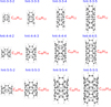 |
Fig. 1. Structures of the hydrogenated nanotubes (hnt) studied in this work. The name of each nanotube is shown above each structure. Where the first two digits are the chiral index, the last digit refers to the number of unit cells of the nanotube. The chemical formulae of the nanotubes are shown to the right of each structure. |
3. Computational method
In this work, the ab initio calculations were carried out using density functional theory (DFT). The dissociation energies and transition state energies were computed using the hybrid density functional B3LYP (Becke 1992; Lee et al. 1988), as implemented in the Gaussian 16 program (Frisch et al. 2016). All structures were optimized using the 6-311++G(2d,p) basis set. It has been reported that such a combination of functional and basis sets, namely, B3LYP/6-311++G(2d,p), produces reasonable ionization, dissociation, and transition state energies for PAHs, and the calculated results are consistent with high-accuracy methods, for example, the CBS-QB3 method (Holm et al. 2011; Johansson et al. 2011; Chen et al. 2015). To take the intermolecular forces into account, the D3 version of Grimme’s dispersion with Becke–Johnson damping (Grimme et al. 2011) is included in the calculations.
The vibrational frequencies are calculated for the optimized geometries to verify that these correspond to minima or first-order saddle points (transition states) on the potential energy surface (PES). The zero point vibrational energies (ZPVE) are taken into account. Intrinsic reaction coordinate (IRC) calculations (Fukui 1981; Dykstra 2005) are performed to confirm that the transition state structures are connected to their corresponding local PES minima. We focus on neutral and cation systems with the lowest multiplicities and only the ground state PES are considered, as the non-radiative decay for such a large molecule is very rapid: ∼10−12 s (Vierheilig et al. 1999; Zewail 2000).
The harmonic IR spectra were calculated with a smaller basis set, viz. B3LYP/6-31+G(d), based on the optimized structures obtained at the same level of theory. Such a combination produces accurate vibrational spectra – previous studies have shown that larger basis sets, could not improve the spectra significantly (Merrick et al. 2007). To achieve more accurate IR spectra, anharmonic effects should be taken into account, which would appreciably affect the number of bands, band positions and relative intensities (Mackie et al. 2015; Chen 2018a).
4. Synthesizing carbon nanotubes through hydrogen-abstraction and acetylene-addition
The hydrogen-abstraction/acetylene-addition (HACA) has been suggested as a formation mechanism of PAHs in the outflows of carbon-rich asymptotic giant branch (AGB) stars (Frenklach et al. 1985; Frenklach & Feigelson 1989; Richter & Howard 2000; Frenklach 2002). In the HACA mechanism, a repetitive hydrogen loss from the aromatic hydrocarbon is followed by addition of one or two acetylene molecule(s) before cyclization and aromatization (Frenklach et al. 1985; Frenklach & Feigelson 1989; Richter & Howard 2000; Appel et al. 2000). Using HACA, Parker et al. (2014) demonstrated in crossed molecular beam experiments combined with electronic structure and quantum-statistical calculations that naphthalene (C10H8) can be synthesized via successive reactions of the phenyl radical with two acetylene molecules. Yang et al. (2017) showed that phenanthrene (C14H10) can also be formed by the reaction of the biphenylyl radical (C12H9•) with a single acetylene molecule through addition to the radical site, followed by cyclization and aromatization. Very recently, Zhao et al. (2018) found a facile, isomer-selective formation pathway of pyrene (C16H10) using the HACA method, and they suggested that molecular mass growth from pyrene may lead through systematic ring expansions, not only to more complex PAHs, but ultimately to 2D graphene-type structures. However, the validity of HACA to form 3D nanostructures has remained uncharted.
Figure 2 shows the molecular mass growth process from planar to 3D structures involving HACA: at the beginning, a benzene combines with a phenyl to form a biphenyl through hydrogen abstraction. Then, the biphenyl loses a hydrogen atom and reacts with another phenyl to form a triphenyl. Following a H-loss, the triphenyl isomerizes to a closed 3D structure, hnt-3-3-1. Subsequently, the molecule may grow to more complex nanotubes following processes similar to the HACA for PAHs (Yang et al. 2017; Zhao et al. 2018).
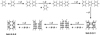 |
Fig. 2. Molecular growth process of 3D nanostructures involving HACA. |
Multiple barriers exist in the proposed formation pathway shown in Fig. 2. Using DFT, we studied the key barriers (transition states) along the formation pathway. Figure 3 shows the formation of biphenyl from two neutral benzenes. The calculated electronic, zero-point vibrational, and total energies of the main strutures are given in the appendix. The reaction pathway begins with the loss of a hydrogen atom from a benzene molecule. A phenyl molecule is formed following the H-loss from benzene, which could clusterize with a neighboring benzene through van der Waals forces. The binding energy of the weakly bonded cluster is found to be 0.13 eV. After that, a 0.18 eV barrier (shown as TS1 in Fig. 3) has to be overcome to form a covalent bond between the phenyl and benzene molecules. To prove the nature of the transition state, we exhibit the imaginary frequency and displacement vectors of the transition state. As shown in Fig. 3, the intensity of the imaginary frequency is about i284 cm−1. The displacement vectors show that the “bald” carbon (without attached hydrogen) on the phenyl side interacts with a carbon on the benzene side, which clearly indicates the tendency to form a covalent bond in between the two carbons. In order to confirm the transition state calculations, we have also investigated the intrinsic reaction coordinates (IRC) transition state, see the appendix for details. In addition, both experimental and theoretical studies have confirmed that the formation of covalent bond in PAH or fullerene clusters could occur efficiently in the interstellar conditions (Zettergren et al. 2013; Zhen et al. 2018; Chen 2018b).
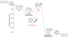 |
Fig. 3. Calculated reaction barriers and dissociation energies for formation of biphenyl from two benzene molecules. The energies are calculated based on the left system (phenyl + benzene). The arrow indicates the intensities of the imaginary frequencies and displacement vectors of the transition state. |
A biphenyl could be formed following the loss of the “extra” hydrogen in between phenyl and benzene (see Fig. 3 for the location of the hydrogen). This process can be repeated to form terphenyl or other larger 2D nanostructures (Yang et al. 2017; Zhao et al. 2018). However, it is unclear how the closed 3D nanostructures could be produced. We find that the molecular bending or curvature is crucial for the formation of 3D geometries (Chen et al. 2017b). Moreover, it has been shown that linear molecules do bend significantly at vibrationally-excited states without breaking the bonds (Chen & Luo 2019). Figure 4 shows the key transition state for the molecule bending, in which a terphenyl converts to a closed 3D nanostructure following the loss of two hydrogens. The imaginary frequency for such transition state is about i476 cm−1. The displacement vectors show that the atoms on both edges of the molecule wag simultaneously towards or away from each other, which demonstrates the tendency to close the structure. Figure A.2 shows the IRC of the barrier for molecular bending (TS2 in Fig. 4). The highest point of the IRC represents the transition state, the left side is the closed nanostructure, while the right side corresponds to the open one (after optimization). One can see that this IRC provides reasonable reaction pathway between the reactant and the product.
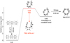 |
Fig. 4. Calculated reaction barrier for molecular bending. The energies are calculated based on the left molecule (terphenyl-H). The arrow indicates the intensity of the imaginary frequency and displacement vector of the transition state. |
Starting from the closed 3D nanostructure (e.g. hnt-3-3-1), The acetylene addition on hydrogenated nanotubes takes about four steps; (i) H-loss from the edge of the HNT, (ii) an acetylene overcomes a barrier (TS3 in Fig. 5) to form a covalent bond with the HNT, (iii) it goes through another barrier (TS4 in Fig. 5) to form a closed hexagon structure, (iv) the dissociation of the “extra” hydrogen (see Fig. 5 for the location of the hydrogen). Following these four steps, the molecule can grow longer and more complex.
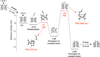 |
Fig. 5. Calculated reaction barriers and dissociation energies for molecular growth process in the 3D nanostructure (hnt-3-3-1). The energies are calculated based on the left system. The arrows indicate the intensities of the imaginary frequencies and displacement vectors of the corresponding transition states. |
5. Infrared vibrational spectra of carbon nanotubes
Figure 6 shows the DFT-calculated spectra of NTs, HNTs and their cations in the spectral range of 3–20 μm. The typical IR bands are also listed in Table 1 and compared with other carbon compounds of astrophysical interest, including PAHs, fullerene, and a graphene sheet. For each transition, we assign a full width at half maximum (FWHM) of 30 cm−1, which is consistent with the natural line width expected from free–flying molecules (Allamandola et al. 1989; Bauschlicher et al. 2008; Boersma et al. 2011; Ricca et al. 2012). This natural line width arises from intramolecular vibrational energy redistribution.
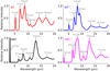 |
Fig. 6. DFT-computed IR vibrational spectra (convolved with Gaussian profiles of FWHM of 30 cm−1) of NTs, HNTs and their cations. |
Dominant IR features of carbon compounds of astrophysical interest.
The molecules included in Fig. 6 are: nt-3-3-2, nt-3-3-3, nt-3-3-4, nt-3-3-5, nt-4-4-2, nt-4-4-3, nt-4-4-4, nt-4-4-5, nt-5-5-2, nt-5-5-3, nt-5-5-4, and nt-5-5-5, as well as their cations. Also included in Fig. 6 are the hydrogenated counterparts of these neutral and cationic NTs. For these 48 spectra, the vibrational bands mostly lay at about 3.3, 5.3, 6.0–9.4, 10.6, 12–15 and 16–18 μm. We obtained the mean spectra of NTs and HNTs by averaging the individual spectrum of each species on a per carbon atom basis, and found that the dominant bands are at ∼5.3, 7.0, 8.8, 9.7, 10.9, 14.2, and 16.8 μm for NTs, and at ∼3.3, 6.5, 8.2, 10.8, 13, and 17.2 μm for HNTs, respectively. For their cationic counterparts, the major bands occur at ∼5.2, 7.1, 8.3, 9.2, 13.4, and 16.7 μm for NT cations, and at ∼3.3, 6.6, 8.3, 10.6, 12.8, and 17.2 μm for HNT cations, respectively. Most noticeably, the 5.3 μm band associated with the C=C symmetric stretching modes on the edge of NTs is absent in HNTs and other carbon compounds of astrophysical interest (see Table 1 for details), while HNTs exhibit a prominent C–H stretching band at 3.3 μm and a prominent C–H out-of-plane bending band at 12.8–13 μm. The later two bands (3.3 and 12.8–13 μm) are rather similar to the UIE bands (3.3 and 12.7 μm), which are commonly attributed to the C–H stretching and C–H out-of-plane bending of PAHs. In addition, the C–C stretching bands at 6.5–6.6 μm and 8.2–8.3 μm of HNTs are also close to the 6.2, 7.7, and 8.6 μm UIE bands. Although some of these bands are difficult to disentangle from the UIE bands, the unprecedented sensitivity of the James Webb Space Telescope (JWST), scheduled to be launched in 2021, will place the detection (or non-detection) of the bands at ∼5.3, 6.5–6.6, 7–7.1, 8.2–8.3, 10.6–10.8, 12.8–13.4, 14.2, and 16.8–17.2 μm on firm ground, and enable far more detailed band analysis and formation pathway than previously possible. The theoretical IR spectra of both neutral and cationic NTs and their hydrogenated counterparts could also be used for possible searches of these species in the ISM with exisiting observations made by, for example, the Infrared Space Observatory and the Spitzer Space Telescope.
6. Summary
Using DFT, we have demonstrated that CNTs could form in the ISM through the hydrogen abstraction and acetylene addition mechanism. CNTs and hydrogenated CNTs, as well as their cationic counterparts, exhibit intense vibrational transitions in the IR. The possible presence of these species in space are to be tested by the upcoming JWST.
Acknowledgments
We thank the anonymous referee for his/her very helpful comments which considerably improved the presentation of this work. We also thank Shaoqi Zhan for sharing his insights on transition state calculations. This work is supported by the Swedish Research Council (Contract No. 2015–06501). The calculations were performed on resources provided by the Swedish National Infrastructure for Computing (SNIC) at the High Performance Computing Center North (HPC2N). A. L. is supported in part by NSF AST–1816411 and NASA 80NSSC19K0572.
References
- Allamandola, L., Tielens, A., & Barker, J. 1989, ApJS, 71, 733 [NASA ADS] [CrossRef] [Google Scholar]
- Appel, J., Bockhorn, H., & Frenklach, M. 2000, Combust. Flame, 121, 122 [CrossRef] [Google Scholar]
- Bauschlicher, Jr., C. W., Peeters, E., & Allamandola, L. J. 2008, ApJ, 678, 316 [NASA ADS] [CrossRef] [Google Scholar]
- Becke, A. D. 1992, J. Chem. Phys., 96, 2155 [NASA ADS] [CrossRef] [Google Scholar]
- Berné, O., & Tielens, A. G. 2012, Proc. Natl. Acad. Sci., 109, 401 [NASA ADS] [CrossRef] [Google Scholar]
- Berne, O., Mulas, G., & Joblin, C. 2013, A&A, 550, L4 [NASA ADS] [CrossRef] [EDP Sciences] [Google Scholar]
- Berné, O., Cox, N., Mulas, G., & Joblin, C. 2017, A&A, 605, L1 [NASA ADS] [CrossRef] [EDP Sciences] [Google Scholar]
- Boersma, C., Bauschlicher, Jr., C., Ricca, A., et al. 2011, ApJ, 729, 64 [NASA ADS] [CrossRef] [Google Scholar]
- Cami, J., Bernard-Salas, J., Peeters, E., & Malek, S. E. 2010, Science, 329, 1180 [NASA ADS] [CrossRef] [PubMed] [Google Scholar]
- Chen, T. 2018a, ApJS, 238, 18 [NASA ADS] [CrossRef] [Google Scholar]
- Chen, T. 2018b, ApJ, 866, 113 [NASA ADS] [CrossRef] [Google Scholar]
- Chen, T., & Luo, Y. 2019, MNRAS, 486, 1875 [NASA ADS] [CrossRef] [Google Scholar]
- Chen, T., Gatchell, M., Stockett, M. H., et al. 2015, J. Chem. Phys., 142, 144305 [NASA ADS] [CrossRef] [Google Scholar]
- Chen, X., Li, A., & Zhang, K. 2017a, ApJ, 850, 104 [NASA ADS] [CrossRef] [Google Scholar]
- Chen, T., Zhen, J., Wang, Y., Linnartz, H., & Tielens, A. G. 2017b, Chem. Phys. Lett., 692, 298 [Google Scholar]
- Cruz-Silva, R., Araki, T., Hayashi, T., et al. 2016, Phil. Trans. R. Soc. A: Math. Phys. Eng. Sci., 374, 20150327 [NASA ADS] [CrossRef] [Google Scholar]
- Dykstra, C. E. 2005, Theory and Applications of Computational chemistry: the First Forty Years (Amsterdam: Elsevier) [Google Scholar]
- Frenklach, M. 2002, Phys. Chem. Chem. Phys., 4, 2028 [Google Scholar]
- Frenklach, M., & Feigelson, E. D. 1989, ApJ, 341, 372 [NASA ADS] [CrossRef] [Google Scholar]
- Frenklach, M., Clary, D. W., Gardiner, Jr., W. C., & Stein, S. E. 1985, Symp. (Int.) Combust., 20, 887 [CrossRef] [Google Scholar]
- Frisch, M., Trucks, G., Schlegel, H., et al. 2016, Gaussian 16 Revision C.01 (Wallingford CT: Gaussian Inc.) [Google Scholar]
- Fukui, K. 1981, Acc. Chem. Res., 14, 363 [CrossRef] [Google Scholar]
- García-Hernández, D., Manchado, A., García-Lario, P., et al. 2010, ApJ, 724, L39 [NASA ADS] [CrossRef] [Google Scholar]
- García-Hernández, D., Iglesias-Groth, S., Acosta-Pulido, J., et al. 2011, ApJ, 737, L30 [NASA ADS] [CrossRef] [Google Scholar]
- García-Hernández, D. A., Villaver, E., García-Lario, P., et al. 2012, ApJ, 760, 107 [NASA ADS] [CrossRef] [Google Scholar]
- Grimme, S., Ehrlich, S., & Goerigk, L. 2011, J. Comput. Chem., 32, 1456 [Google Scholar]
- Henning, T., & Salama, F. 1998, Science, 282, 2204 [NASA ADS] [CrossRef] [PubMed] [Google Scholar]
- Holm, A. I., Johansson, H. A., Cederquist, H., & Zettergren, H. 2011, J. Chem. Phys., 134, 044301 [NASA ADS] [CrossRef] [PubMed] [Google Scholar]
- Iijima, S. 1991, Nature, 354, 56 [NASA ADS] [CrossRef] [Google Scholar]
- Johansson, H. A., Zettergren, H., Holm, A. I., et al. 2011, J. Chem. Phys., 135, 084304 [NASA ADS] [CrossRef] [Google Scholar]
- Kroto, H., Heath, J., O’brien, S., Curl, R., & Smalley, R. 1985, Nature, 318, 162 [NASA ADS] [CrossRef] [Google Scholar]
- Kwok, S., & Zhang, Y. 2011, Nature, 479, 80 [NASA ADS] [CrossRef] [PubMed] [Google Scholar]
- Lee, C., Yang, W., & Parr, R. G. 1988, Phys. Rev. B, 37, 785 [Google Scholar]
- Leger, A., & Puget, J. 1984, A&A, 137, L5 [NASA ADS] [Google Scholar]
- Li, A., & Mann, I. 2012, Nanodust in the Solar System: Discoveries and Interpretations (Berlin: Springer), 5 [NASA ADS] [CrossRef] [Google Scholar]
- Mackie, C. J., Candian, A., Huang, X., et al. 2015, J. Chem. Phys., 143, 224314 [NASA ADS] [CrossRef] [Google Scholar]
- Merrick, J. P., Moran, D., & Radom, L. 2007, J. Phys. Chem. A, 111, 11683 [CrossRef] [PubMed] [Google Scholar]
- Parker, D. S., Kaiser, R. I., Troy, T. P., & Ahmed, M. 2014, Angew. Chem., 126, 7874 [CrossRef] [Google Scholar]
- Pendleton, Y. J., & Allamandola, L. J. 2002, ApJS, 138, 75 [NASA ADS] [CrossRef] [Google Scholar]
- Pietrucci, F., & Andreoni, W. 2014, J. Chem. Theory Comput., 10, 913 [CrossRef] [Google Scholar]
- Ricca, A., Bauschlicher, Jr., C. W., Boersma, C., Tielens, A. G., & Allamandola, L. J. 2012, ApJ, 754, 75 [NASA ADS] [CrossRef] [Google Scholar]
- Richter, H., & Howard, J. B. 2000, Combust. Sci., 26, 565 [Google Scholar]
- Sellgren, K., Werner, M. W., Ingalls, J. G., et al. 2010, ApJ, 722, L54 [NASA ADS] [CrossRef] [Google Scholar]
- Strelnikov, D., Kern, B., & Kappes, M. 2015, A&A, 584, A55 [NASA ADS] [CrossRef] [EDP Sciences] [Google Scholar]
- Terrones, H., Terrones, M., López-Urías, F., Rodríguez-Manzo, J. A., & Mackay, A. L. 2004, Phil. Trans. R. Soc. London Ser. A: Math. Phys. Eng. Sci., 362, 2039 [CrossRef] [Google Scholar]
- Uberuaga, B. P., Stuart, S. J., Windl, W., Masquelier, M. P., & Voter, A. F. 2012, Comput. Theoret. Chem., 987, 115 [CrossRef] [Google Scholar]
- Vierheilig, A., Chen, T., Waltner, P., et al. 1999, Chem. Phys. Lett., 312, 349 [CrossRef] [Google Scholar]
- Yang, T., Kaiser, R. I., Troy, T. P., et al. 2017, Angew. Chem., 129, 4586 [CrossRef] [Google Scholar]
- Zettergren, H., Rousseau, P., Wang, Y., et al. 2013, Phys. Rev. Lett., 110, 185501 [NASA ADS] [CrossRef] [PubMed] [Google Scholar]
- Zewail, A. H. 2000, J. Phys. Chem. A, 104, 5660 [CrossRef] [Google Scholar]
- Zhao, L., Kaiser, R. I., Xu, B., et al. 2018, Nat. Astron., 2, 413 [CrossRef] [Google Scholar]
- Zhen, J., Castellanos, P., Paardekooper, D. M., Linnartz, H., & Tielens, A. G. 2014, ApJ, 797, L30 [NASA ADS] [CrossRef] [Google Scholar]
- Zhen, J., Chen, T., & Tielens, A. G. G. M. 2018, ApJ, 863, 128 [NASA ADS] [CrossRef] [Google Scholar]
Appendix A: Additional figures
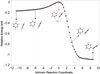 |
Fig. A.1. Intrinsic reaction coordinates (IRC) for the transition state of TS1 (see Fig. 3). The arrows indicate the structures at the corresponding IRC steps. |
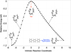 |
Fig. A.2. IRC for transition state of TS2 (see Fig. 4). The structure in the bottom-right corner represents the optimized geometry of the right–end IRC step. |
 |
Fig. A.5. DFT calculations (B3LYP/6-311++G(2d,p)) of electronic, zero point vibrational and total energies of studied molecules. The values are given in eV. |
All Tables
All Figures
|
Fig. 1. Structures of the hydrogenated nanotubes (hnt) studied in this work. The name of each nanotube is shown above each structure. Where the first two digits are the chiral index, the last digit refers to the number of unit cells of the nanotube. The chemical formulae of the nanotubes are shown to the right of each structure. |
| In the text | |
|
Fig. 2. Molecular growth process of 3D nanostructures involving HACA. |
| In the text | |
|
Fig. 3. Calculated reaction barriers and dissociation energies for formation of biphenyl from two benzene molecules. The energies are calculated based on the left system (phenyl + benzene). The arrow indicates the intensities of the imaginary frequencies and displacement vectors of the transition state. |
| In the text | |
|
Fig. 4. Calculated reaction barrier for molecular bending. The energies are calculated based on the left molecule (terphenyl-H). The arrow indicates the intensity of the imaginary frequency and displacement vector of the transition state. |
| In the text | |
|
Fig. 5. Calculated reaction barriers and dissociation energies for molecular growth process in the 3D nanostructure (hnt-3-3-1). The energies are calculated based on the left system. The arrows indicate the intensities of the imaginary frequencies and displacement vectors of the corresponding transition states. |
| In the text | |
|
Fig. 6. DFT-computed IR vibrational spectra (convolved with Gaussian profiles of FWHM of 30 cm−1) of NTs, HNTs and their cations. |
| In the text | |
|
Fig. A.1. Intrinsic reaction coordinates (IRC) for the transition state of TS1 (see Fig. 3). The arrows indicate the structures at the corresponding IRC steps. |
| In the text | |
|
Fig. A.2. IRC for transition state of TS2 (see Fig. 4). The structure in the bottom-right corner represents the optimized geometry of the right–end IRC step. |
| In the text | |
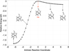 |
Fig. A.3. IRC for transition state of TS3 (see Fig. 5). |
| In the text | |
 |
Fig. A.4. IRC for transition state of TS4 (see Fig. 5). |
| In the text | |
|
Fig. A.5. DFT calculations (B3LYP/6-311++G(2d,p)) of electronic, zero point vibrational and total energies of studied molecules. The values are given in eV. |
| In the text | |
Current usage metrics show cumulative count of Article Views (full-text article views including HTML views, PDF and ePub downloads, according to the available data) and Abstracts Views on Vision4Press platform.
Data correspond to usage on the plateform after 2015. The current usage metrics is available 48-96 hours after online publication and is updated daily on week days.
Initial download of the metrics may take a while.