| Issue |
A&A
Volume 630, October 2019
|
|
|---|---|---|
| Article Number | A113 | |
| Number of page(s) | 8 | |
| Section | Extragalactic astronomy | |
| DOI | https://doi.org/10.1051/0004-6361/201936354 | |
| Published online | 01 October 2019 | |
Stellar systems following the R1/m luminosity law
IV. The total energy and the central concentration of galaxies
1
Sterrenkundig Observatorium, Universiteit Gent, Krijgslaan 281 S9, 9000 Gent, Belgium
e-mail: This email address is being protected from spambots. You need JavaScript enabled to view it.
2
Dipartimento di Fisica e Astronomia, Università di Bologna, Via Piero Gobetti 93/2, Bologna, Italy
Received:
22
July
2019
Accepted:
2
September
2019
Abstract
We expand our previous analytical and numerical studies of the family of Sérsic models, which are routinely used to describe early-type galaxies and the bulges of spiral galaxies. In particular, we focus on the total energy budget, an important dynamical property that has not been discussed in detail in previous works. We use two different methods to calculate the total energy for the Sérsic model family that result in two independent expressions that can be used along the entire sequence of Sérsic models. We use these expressions to investigate whether the Spitzer concentration index is a reliable measure for the intrinsic 3D concentration of galaxies, and we conclude that it is not a very useful measure for the central concentration. The popular Third Galaxy Concentration index, on the other hand, is shown to be a reliable measure for the intrinsic 3D concentration, even though it is based on the surface brightness distribution and not on the intrinsic 3D density.
Key words: galaxies: structure / galaxies: kinematics and dynamics / methods: analytical
© ESO 2019
1. Introduction
Over the past decades, the Sérsic model has become the preferred model to describe the surface brightness profiles of early-type galaxies and spiral galaxies bulges (e.g. Davies et al. 1988; Caon et al. 1993; Möllenhoff & Heidt 2001; Graham & Guzmán 2003; Allen et al. 2006; Gadotti 2009; Bruce et al. 2012; Kelvin et al. 2012; van der Wel et al. 2012; Salo et al. 2015; Lange et al. 2016). The model is the prime component of all modern galaxy profile fitting codes (Peng et al. 2002, 2010; Mosenkov 2014; Erwin 2015; Robotham et al. 2017). It is hence not surprising that the properties of the Sérsic model have been examined in great detail in the past three decades.
As the model is defined by means of the surface brightness profile, many of the projected, that is, on-sky, properties can be expressed analytically (Ciotti 1991; hereafter Paper I; Ciotti & Bertin 1999; Trujillo et al. 2001). A compendium of the most important photometric properties has been presented by Graham & Driver (2005), and the gravitational lensing characteristics are discussed by Cardone (2004) and Elíasdóttir & Möller (2007).
A disadvantage of the Sérsic model is that the standard Abel deprojection of the surface brightness profile does not yield a closed expression for the density in terms of elementary functions or even in terms of standard special functions. Several authors proposed approximations for the spatial density of the Sérsic model (Prugniel & Simien 1997; Lima Neto et al. 1999; Trujillo et al. 2002a). It was found that closed expressions for the density and related properties can be derived using Mellin integral transforms. The resulting expressions are written in terms of the Fox H function, or the Meijer G function for integer and half-integer values of m (Mazure & Capelato 2002; Baes & Gentile 2011; Baes & Van Hese 2011).
The dynamical properties of the Sérsic model were first investigated in the first two papers of this series (Paper I; Ciotti & Lanzoni 1997; hereafter Paper II). These papers focused on relatively large Sérsic indices (m ⩾ 2). These studies were extended by Baes & Ciotti (2019); hereafter Paper III, where we considered the entire range of Sérsic indices, and particularly focused on small values of m, appropriate for low-mass and dwarf ellipticals. An important result of these studies is that all Sérsic models with  can be supported by an isotropic velocity dispersion tensor, and that these isotropic models are stable to both radial and non-radial perturbations. Sérsic models with smaller values of m, however, cannot be supported by an isotropic velocity dispersion tensor.
A dynamical property of the Sérsic models that has not been discussed analytically is their total energy. For example, the total energy budget of an equilibrium dynamical model is relevant for numerical studies, as it sets the preferred length scale for Monte Carlo or N-body simulations. The need for a consistent set of standard units for cluster simulations has been advocated since the 1970s, and the most popular system that has emerged is the system of so-called standard N-body units (Hénon 1971; Cohn 1979; Heggie & Mathieu 1986)1. This unit system is defined by the requirements G = M = 1,  , or equivalently, uses the virial radius as the length unit.
Moreover, from the theoretical point of view, the total energy budget is one of the ingredients required to calculate the concentration parameter introduced by Spitzer (1969). Contrary to other concentration indices (e.g. Trujillo et al. 2001; Graham et al. 2001a; Aswathy & Ravikumar 2018), it is based on the intrinsic 3D density distribution, rather than on the light distribution on the plane of the sky. In the past few years, the interest in the central light (or mass) concentration of galaxies has only increased, thanks to a number of scaling relations between the central concentration and other galactic parameters, including velocity dispersion, supermassive black hole mass, optical-to-X-ray flux ratio and nuclear radio emission (e.g. Graham et al. 2001a,b; Pović et al. 2009; Aswathy & Ravikumar 2018). If physical processes in the evolution of a galaxy affect the mass or light concentration in a galaxy, we would primarily expect correlations that involve concentration indices based on the intrinsic density. It does therefore make sense to investigate the relation between intrinsic and projected concentration indices for the Sérsic model, in particular for the low-m regime where the intrinsic density distribution shows interesting characteristics (Paper III).
The goal of our study is twofold. Firstly, we wish to extend the body of analytical studies on the Sérsic model by providing a closed expression for the total energy. Secondly, we use these expressions to compare the intrinsic Spitzer concentration index to the commonly used the Third Galaxy Concentration (TGC) light concentration index (Trujillo et al. 2001) to find out how we can best parameterise the intrinsic 3D concentration. In Sect. 2 we summarise some general properties of the family of Sérsic models. In Sect. 3 we compute the total energy of the family of Sérsic models using two different approaches: the strip brightness approach, and the Mellin integral transform framework. In Sect. 4 we use these results to compare 2D and 3D concentration indices for the Sérsic model, and we compare the Sérsic model with other popular families of spherical dynamical models. Our results are summarised in Sect. 5.
2. Sérsic model
The Sérsic model is defined by the surface brightness profile
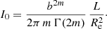
![Mathematical equation: $$ \begin{aligned} I(R) = I_0\exp \left[-b\left(\frac{R}{R_{\text{e}}}\right)^{1/m}\right]. \end{aligned} $$](/articles/aa/full_html/2019/10/aa36354-19/aa36354-19-eq3.gif) (1)
(1)
It is a three-parameter family with I0 the central surface brightness, Re the effective radius, and m the so-called Sérsic index. The parameter b = b(m) is not a free parameter in the model, but a dimensionless parameter that is set such that Re corresponds to the isophote that contains half of the emitted luminosity. For a given m, the corresponding value of b can be found by solving a non-algebraic equation, and various interpolation formulae have been presented in the literature (Capaccioli 1989; Prugniel & Simien 1997; MacArthur et al. 2003; Paper I; Paper III). In particular, we recall the exact asymptotic formulae for large and small values of m (Ciotti & Bertin 1999, Paper III).
Instead of the central surface brightness I0, we can also use the total luminosity L as a free parameter. The connection between both quantities is
 (2)
(2)
For more formulae related to the Sérsic model, and for figures illustrating how the most important properties vary as a function of m, we refer to Paper I, Paper III, and Graham & Driver (2005).
3. Total energy of the Sérsic model
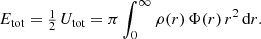
For a spherically symmetric system characterised by a mass density ρ(r) and a gravitational potential Φ(r), the expression for the total energy Etot is given by
 (3)
(3)
In this expression, Utot represents the total potential energy of the system, and the equality  is a manifestation of the virial theorem (e.g. Binney & Tremaine 2008). An alternative expression for Etot is based on the cumulative mass density M(r) instead of the gravitational potential,
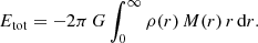 (4)
(4)
Considering that the spatial density of the Sérsic model, obtained from an Abel inversion of Eq. (1), is not an elementary function (which means that this is even less true for the derived quantities such as the potential and the cumulative mass), and that the two integrals above involve products of these functions, it seems natural that the only approach to their evaluation is numerical integration. Starting from the surface brightness profile, Expressions (3) and (4) are five-dimensional and four-dimensional integrals, respectively. In the following we show that it is possible to obtain two different expressions for the total energy using the strip brightness quantity introduced by Schwarzschild (1954) and by direct integration using advanced special functions.
3.1. Calculation using the strip brightness
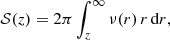
A first method for calculating the total energy uses the strip brightness 𝒮(z), a quantity defined so that 𝒮(z) dz is the total luminosity in a strip of width dz on the plane of the sky that passes a distance z from the centre of the system. For a spherically symmetric system, the strip brightness can be written as (Schwarzschild 1954)
 (5)
(5)
where ν(r) is the luminosity density. An equivalent expression for 𝒮(z) is
 (6)
(6)
The equivalence of these two expression can easily be demonstrated by inserting the projection equation
 (7)
(7)
into Expression (6) and changing the order of the resulting double integral (see also Binney & Tremaine 2008, Problem 1.3).
Schwarzschild (1954) demonstrated that Etot can be calculated from the strip brightness using
 (8)
(8)
with Υ the mass-to-light ratio of the system. We now elaborate on the previous identity, following a path apparently unnoticed in Schwarzschild (1954). We first obtain a generic 2D integral expression for Etot in terms of the surface brightness profile, and in the special case of the Sérsic profile we then show that the integral can be reduced to a 1D integral. We proceed as follows. Inserting Eq. (6) into (8), we find a triple integral
 (9)
(9)
Changing the order of integrations, we find after some calculation
 (10)
(10)
with 𝕂(k) the complete elliptic integral of the first kind, and with the definition
 (11)
(11)
Up to now, we have used generic formulae and have not yet used the specific form of the Sérsic surface brightness profile. This expression shows that when the strip brightness function introduced by Schwarzschild (1954) and repeated exchanges in the integration order are used, the total energy of any generic spherical model defined by a surface brightness density I(R) can always be reduced to a 2D integral. Interestingly, for the Sérsic model, one of the two integrals can be evaluated analytically. Indeed, with Expression (1), f(ϕ) becomes
![Mathematical equation: $$ \begin{aligned} f(\phi ) = I_0^2 \int _0^\infty \exp \left[-b\left(\frac{R}{R_{\text{e}}}\right)^{1/m}\Omega \right] R^2\,{\text{d}}R = \frac{I_0^2\,R_{\text{e}}^3 m\,\Gamma (3m)}{b^{3m}\,\Omega ^{3m}},\end{aligned} $$](/articles/aa/full_html/2019/10/aa36354-19/aa36354-19-eq15.gif) (12)
(12)
with the quantity Ω defined as Ω = cos1/mϕ + sin1/mϕ. Inserting this expression into Eq. (10) reduces the expression for the total energy to a relatively single expression that involves just a single integration. Setting k = tanϕ, and using Expression (2), we obtain
 (13)
(13)
with M = Υ L the total mass of the system. Many different integrals of the complete elliptic integral of the first kind can be evaluated exactly (e.g. Glasser 1976; Cvijovic & Klinowski 1999; Gradshteyn et al. 2007). Unfortunately, the integral in Expression (13) is not found among these lists. It is easily evaluated numerically, however, as the integrand is well behaved over the entire integration domain.
3.2. Calculation using advanced special functions
A second method for calculating Etot for the Sérsic model is using the analytical expressions for the density and related properties derived by Baes & Gentile (2011) and Baes & Van Hese (2011) in terms of the Fox H function. The general expression for the density is (Paper III)
![Mathematical equation: $$ \begin{aligned} \rho (r) = \frac{b^{3m}}{\pi ^{3/2}\,\Gamma (2m)}\,\frac{M}{R_{\text{e}}^3}\,u^{-1}\, H^{2,0}_{1,2} \left[ \left.\begin{matrix} (0,1) \\ (0,2m), \left(\tfrac{1}{2},1\right) \end{matrix} \,\right| u^2 \right], \end{aligned} $$](/articles/aa/full_html/2019/10/aa36354-19/aa36354-19-eq17.gif) (14)
(14)
where we have used the dimensionless spherical radius
 (15)
(15)
The corresponding mass profile is
![Mathematical equation: $$ \begin{aligned} M(r) = \frac{2M}{\sqrt{\pi }\, \Gamma (2m)}\,u^2\, H^{2,1}_{2,3} \left[ \left.\begin{matrix} (0,1), (0,1) \\ (0,2m), \left(\tfrac{1}{2},1\right), (-1,1) \end{matrix}\,\right| u^2 \right]\cdot \end{aligned} $$](/articles/aa/full_html/2019/10/aa36354-19/aa36354-19-eq19.gif) (16)
(16)
When we substitute Expressions (14) and (16) in definition (3), we find the total energy
![Mathematical equation: $$ \begin{aligned} E_{\text{tot}} =&-\frac{b^m}{2\pi \, \Gamma ^2(2m)}\,\frac{GM^2}{R_{\text{e}}} \nonumber \\&\times \int _0^\infty H^{2,1}_{2,3}\left[\left.\begin{matrix} (0,1), (0,1) \\ (0,2m), (-\tfrac{1}{2},1), (-1,1) \end{matrix}\,\right| z \right] \nonumber \\&\times H^{2,0}_{1,2}\left[\left.\begin{matrix} (0,1) \\ (0,2m), (\tfrac{1}{2},1) \end{matrix}\,\right| z \right] z^{1/2}\, {\text{d}}z. \end{aligned} $$](/articles/aa/full_html/2019/10/aa36354-19/aa36354-19-eq20.gif) (17)
(17)
This integral can be evaluated using the standard integration formula for a product of two Fox H functions (Mathai et al. 2009), and after some simplifications, we obtain
![Mathematical equation: $$ \begin{aligned} E_{\text{tot}} =&-\frac{b^m}{2\pi \, \Gamma ^2(2m)}\,\frac{GM^2}{R_{\text{e}}} \nonumber \\&\times H^{2,2}_{3,3} \left[\left.\begin{matrix} (1-3m,2m),(0,1),(0,1) \\ (0,2m), (-\tfrac{1}{2},1), (-\tfrac{1}{2},1) \end{matrix} \,\right| 1 \right]. \end{aligned} $$](/articles/aa/full_html/2019/10/aa36354-19/aa36354-19-eq21.gif) (18)
(18)
For integer and half-integer values of m, the Fox H function in Expression (18) can be reduced to Meijer G functions. This reduction is based on the integral representations of the Meijer G and Fox H function, and Gauss’ multiplication theorem. The result reads
![Mathematical equation: $$ \begin{aligned} E_{\text{tot}} =&-\frac{(2m)^{3m-1}\,b^m}{(2\pi )^{2m}\,\Gamma ^2(2m)}\,\frac{GM^2}{R_{\text{e}}}\, \nonumber \\&\times G^{2m,2m}_{2m,2m} \!\left[\left. \begin{matrix} -\tfrac{m+1}{2m},-\tfrac{m+2}{2m},\ldots ,-\tfrac{3m-1}{2m},0 \\ \tfrac{1}{2m},\tfrac{2}{2m}\ldots ,\tfrac{2m-1}{2m},-\tfrac{1}{2} \end{matrix} \,\right|1 \right]. \end{aligned} $$](/articles/aa/full_html/2019/10/aa36354-19/aa36354-19-eq22.gif) (19)
(19)
3.3. Numerical values
In Table 1 we tabulate the value of the total energy and the gravitational radius rG, defined through the relation
 (20)
(20)
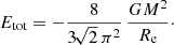
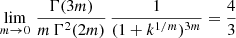
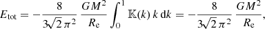
for a number of values between m = 0 and m = 10. These values were calculated through both Expressions (13) and (19) with 15 significant digits, and are found to be in perfect agreement. We also find perfect agreement with the analytical results for the few special cases for which Etot can be calculated analytically, that is, for m = 0,  and 1 (Appendix A). We therefore conclude that both the expressions are equivalent, or that the integral in Eq. (13) can be evaluated exactly as
![Mathematical equation: $$ \begin{aligned}&\int _0^1 \frac{{\mathbb{K} }(k)\,k\,{\text{d}}k}{(1+k^{1/m})^{3m}}=\frac{\pi \,m}{4\,\Gamma (3m)} H^{2,2}_{3,3} \left[\left.\begin{matrix} (1-3m,2m),(0,1),(0,1) \\ (0,2m), (-\tfrac{1}{2},1), (-\tfrac{1}{2},1) \end{matrix} \,\right| 1 \right]. \end{aligned} $$](/articles/aa/full_html/2019/10/aa36354-19/aa36354-19-eq25.gif) (21)
(21)
Numerical values for the total energy Etot, the gravitational radius rG, the half-mass radius rh, the Spitzer concentration index CS, the TGC concentration index, and the 3D version of the TGC (TGC3D) as a function of m.
The values for Etot for 2 ≤ m ≤ 10 are in good agreement with those listed in Paper I. We obtained them there through numerical integration.
4. Discussion
4.1. Central concentration of the Sérsic models
The calculation of the total energy of the family of Sérsic models is primarily important in the discussion on the central concentration of galaxies. The degree to which light or mass is centrally concentrated is an important diagnostic for galaxies. The importance is obvious when the many physical galaxy properties are considered that correlate with (different measures of) the galaxy light concentration, including total luminosity (Caon et al. 1993; Graham et al. 2001a), velocity dispersion (Graham et al. 2001a), Mg/Fe abundance ratio (Vazdekis et al. 2004), central supermassive black hole mass (Graham et al. 2001b; Aswathy & Ravikumar 2018), cluster local density (Trujillo et al. 2002b), and emission at radio and X-ray wavelengths (Pović et al. 2009; Aswathy & Ravikumar 2018). This has inspired several teams to propose galaxy concentration as an important parameter in automated galaxy classification schemes (Doi et al. 1993; Abraham et al. 1994; Bershady et al. 2000; Conselice 2003).
There are many different ways in which the central concentration of galaxies can be estimated or parameterised. A number of concentration indices, such as the widely used C31 index, are defined as the ratio of radii that contain certain fractions of the total galaxy luminosity (de Vaucouleurs 1977; Kent 1985; Bershady et al. 2000). Other concentration indices are based on the ratio of the luminous flux enclosed by two different apertures (Okamura et al. 1984; Doi et al. 1993). Possibly the most commonly used measure for the central light concentration of galaxies today is the TGC index, introduced by Trujillo et al. (2001) as the ratio between the flux within the isophote at a radius αRe, with α a number between 0 and 1, and the flux within the isophote at Re,
 (22)
(22)
For the family of Sérsic models, the TGC index can be calculated analytically (Trujillo et al. 2001; Graham & Driver 2005),
 (23)
(23)
where γ(s, x) is the lower incomplete gamma function. Expression (23) only depends on α and the Sérsic index m; there is no dependency on effective radius, luminosity, or central surface brightness. In the remainder of this paper, we always use  , the value that is generally adopted (e.g. Trujillo et al. 2001; Graham et al. 2001b; Pasquato & Bertin 2010). We have, however, repeated the entire analysis for different values of α, and have found that our results and conclusions are not sensitive to the particular choice of α.
As has been shown by Trujillo et al. (2001) and Graham et al. (2001a), the TGC index is a monotonically increasing function of m. In the limit of m → 0, the surface brightness profile is a uniform disc on the sky (Paper III), and it is easy to see that  . In Fig. 1 the green line shows the TGC index as a function of the Sérsic index m.
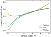 |
Fig. 1. Dependence of the Spitzer concentration index (Eq. (24)), the TGC index (Eq. (23)), and the 3D TGC index (Eq. (25)) on the Sérsic index m. |
A potential caveat of concentration indices such as the C31 or TGC indices is that they are based on the observed, projected distribution of light on the plane of the sky. A physical characterisation of the central concentration of light (or mass) should in principle be based on the intrinsic 3D density distribution. A characterisation that satisfies this requirement is the Spitzer concentration index (Spitzer 1969), defined almost half a centuary ago as the ratio between the half-mass radius and the gravitational radius,
 (24)
(24)
The half-mass radius rh is obviously the radius of the spherical volume that contains half of the total mass, and the gravitational radius is defined through Eq. (20).
Table 2 of Paper I lists numerical approximations for the Spitzer concentration index for a number of Sérsic models with m ⩾ 2. It was noted that CS is an monotonically increasing function of m, as expected. This behaviour does not extend over the entire range of Sérsic indices, however. The yellow line in Fig. 1 shows how CS varies with m between 0 and 10, and numerical values are listed in the fifth column of Table 1. In contrast to the TGC index, Spitzer concentration index is not a monotonically increasing function of m. For m ≳ 1.6 it does increase with increasing m, in agreement with the observation in Paper I. For values of m ≲ 1.6, CS increases again for decreasing m with a rate that is quite steep due to the strong variation of the total energy. At m = 0, a limiting value CS ≈ 0.4943 is reached, which would imply that the constant intensity model would be more centrally concentrated than a de Vaucouleurs model.
A logical consequence is that the TGC and Spitzer concentration indices are not correlated for the family of Sérsic models. In the left panel of Fig. 2 we show the position of the family of Sérsic models in the plane formed by these two indices. The sequence of models forms a banana-shaped trail in this diagram. This diagram suggests that the Spitzer index is a poor metric to indicate the central mass or light concentration in galaxies.
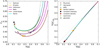 |
Fig. 2. Location of the Sérsic model family, as well as most other popular spherical toy models, in the (TGC, CS) and the (TGC, TGC3D) planes. The models form banana-shaped trails in the former plane, whereas they are located on an almost perfect one-to-one relation in the latter plane. This shows that the Spitzer concentration index is a poor indicator of the intrinsic 3D concentration, whereas the TGC is a very accurate indicator. |
4.2. Comparison to other models
In order to further investigate the usefulness of the Spitzer index as an indicator for the central concentration, we have also calculated the TGC and CS indices for a number of other popular families of toy models that are often used to represent galaxies. These families are also shown in the left panel of Fig. 2. Except for the sequence that corresponds to the Sérsic models, this plot also contains the γ- or Dehnen models (Dehnen 1993; Tremaine et al. 1994), the β-models (Zhao 1996), the Veltmann or hypervirial models (Veltmann 1979; Evans & An 2005), the Einasto models (Einasto 1965; Cardone et al. 2005), and the cored Nuker or Zhao  models (Zhao 1996). Some well-known specific models are also indicated: the Plummer model (Plummer 1911; Dejonghe 1987), Hénon’s isochrone sphere (Henon 1959), the Hernquist model (Hernquist 1990), the Jaffe model (Jaffe 1983), the perfect sphere (de Zeeuw 1985), the Gaussian model (Appendix A.2), the constant density sphere (Binney & Tremaine 2008), and the constant intensity sphere (Paper III). Most of these models belong to one or more of the families mentioned above. In particular, the Hernquist model lies at the intersection of the Veltmann, β- and Dehnen models, the Plummer sphere belongs to the Veltmann and cored Nuker families, and the Gaussian model is common between the Sérsic and Einasto sequences. For all of these models, the total energy budget can be calculated analytically (Appendix B).
It is quite interesting to see that all of these different models occupy a relatively narrow region in the (TGC, CS) plane. This is remarkable, given the large variety in central density slopes between these models, ranging from models with a constant central density to models with a strong density cusp. Furthermore, it is clear that the banana-shaped trail of the Sérsic models is not unique to this specific family of models. On the contrary, it seems to be a general feature: the Veltmann, Einasto, β and cored Nuker models show the same behaviour. Among the models with the lowest CS values are the perfect sphere and Hénon’s isochrone sphere, two models with a central density core and a relatively shallow r−4 fall-off at large radii. It does not make sense that these models, according to this concentration index, would be characterised as less centrally concentrated than the constant intensity sphere, in which the density does increase with increasing radius (Paper III). In conclusion, the Spitzer index is not a very useful measure for the central concentration of dynamical models.
4.3. Intrinsic 3D concentration
If the Spitzer concentration index is not a useful measure for the intrinsic 3D concentration, which index should be used? Based on the monotonic dependence of the TGC index on m for the family of Sérsic models, it might be thought that the TGC index, while defined to measure the concentration of the surface brightness distribution on the sky, is also a suitable measure for the intrinsic 3D concentration. Similarly, for the family of Dehnen models, the TGC index increases monotonically with the central slope γ, which is a natural measure for the central concentration for this family.
To test whether the TGC index is a reliable measure for the intrinsic 3D density concentration, we define a general 3D version of the TGC index as the ratio between the mass contained within a sphere with radius αrh and the mass contained within the half-mass radius rh,
 (25)
(25)
Again we assume  . The blue line in Fig. 1 shows that the TGC3D index varies monotonically as function of m in a way that is very similar to the TGC index.
The right panel of Fig. 2 shows the correlation between the TGC and TGC3D indices, not only for the Sérsic family, but for all the models also shown in the left panel. There is an almost perfect one-to-one correlation between both indices over the different classes of models. For models with a small central concentration, such as the Sérsic models with small m, the TGC3D index is systematically lower than the TGC index. As the models are more and more centrally concentrated, the difference between the two indices becomes smaller, and for very centrally concentrated systems, both indices converge to one. This shows that the TGC index is a reliable measure for the intrinsic 3D concentration, and no separate index such as the TGC3D index needs to be invoked to distinguish between 2D and 3D concentration of galaxies. It therefore makes perfect sense to use the TGC index in statistical studies between global galaxy parameters.
5. Summary
We have expanded our previous analytical and numerical studies of the family of Sérsic models, and concentrated on the total energy budget. The main results of this dedicated study are the following.
Firstly, we explored the Schwarzschild (1954) formalism of the strip brightness to calculate the total energy budget for the Sérsic family. This resulted in a relatively simple expression that involves just a single integration. In a completely independent way, we obtained a closed expression for the total energy in terms of the Fox H function, thanks to the closed expressions for density and related properties derived in our previous work (Baes & Gentile 2011; Baes & Van Hese 2011). In turn, this means that we have a closed-form solution for the 1D integral obtained in the previous approach. We were not able to find this expression in all the standard tables of special functions, and the well-known computer algebra systems were also unable to compute the resulting integral. The two expressions are shown to be in agreement by performing numerical integration. We present a table with values for the total energy budget covering the entire range of Sérsic parameters.
Subsequently, we used our calculations to investigate whether the Spitzer concentration index (Spitzer 1969) is a reliable measure for the intrinsic 3D concentration of galaxies. We find that this is not the case: the index does not correlate with the Sérsic parameter in the low-m range. More generally, we compared the Spitzer concentration index to the popular TGC index (Trujillo et al. 2001) for a wide range of spherical galaxy models, and find that these two indices do not correlate over the entire possible parameter space. We conclude that the Spitzer concentration index is not a very useful measure for the central concentration of dynamical models. On the other hand, we defined a 3D version of the TGC index, and found an almost perfect correlation between the 2D and 3D versions over a wide range of dynamical models. This implies that the TGC index is a reliable measure for the intrinsic 3D concentration, even though it is based on the surface brightness distribution and not on the intrinsic 3D density.
While this study is primarily a theoretical study, it also has a practical use for numerical studies of equilibrium dynamical models because the total energy sets the preferred length scale in the standard or Hénon unit system (Hénon 1971; Heggie & Mathieu 1986).
The use of this unit system has been strongly advocated by Heggie & Mathieu (1986), and as a result, these standard units have sometimes been called Heggie units. In 2014, Douglas Heggie proposed the name Hénon units to commemorate the original proposer.
References
- Abraham, R. G., Valdes, F., Yee, H. K. C., & van den Bergh, S. 1994, ApJ, 432, 75 [NASA ADS] [CrossRef] [Google Scholar]
- Allen, P. D., Driver, S. P., Graham, A. W., et al. 2006, MNRAS, 371, 2 [NASA ADS] [CrossRef] [Google Scholar]
- Aswathy, S., & Ravikumar, C. D. 2018, MNRAS, 477, 2399 [NASA ADS] [CrossRef] [Google Scholar]
- Baes, M., & Ciotti, L. 2019, A&A, 626, A110 [NASA ADS] [CrossRef] [EDP Sciences] [Google Scholar]
- Baes, M., & Gentile, G. 2011, A&A, 525, A136 [NASA ADS] [CrossRef] [EDP Sciences] [Google Scholar]
- Baes, M., & Van Hese, E. 2011, A&A, 534, A69 [NASA ADS] [CrossRef] [EDP Sciences] [Google Scholar]
- Bershady, M. A., Jangren, A., & Conselice, C. J. 2000, AJ, 119, 2645 [NASA ADS] [CrossRef] [Google Scholar]
- Binney, J., & Tremaine, S. 2008, Galactic Dynamics, 2nd edn. (Princeton: Princeton University Press) [Google Scholar]
- Bruce, V. A., Dunlop, J. S., Cirasuolo, M., et al. 2012, MNRAS, 427, 1666 [NASA ADS] [CrossRef] [Google Scholar]
- Caon, N., Capaccioli, M., & D’Onofrio, M. 1993, MNRAS, 265, 1013 [NASA ADS] [CrossRef] [Google Scholar]
- Capaccioli, M. 1989, in World of Galaxies (Le Monde des Galaxies), eds. H. G. Corwin, Jr., & L. Bottinelli, 208 [CrossRef] [Google Scholar]
- Cardone, V. F. 2004, A&A, 415, 839 [NASA ADS] [CrossRef] [EDP Sciences] [Google Scholar]
- Cardone, V. F., Piedipalumbo, E., & Tortora, C. 2005, MNRAS, 358, 1325 [NASA ADS] [CrossRef] [Google Scholar]
- Ciotti, L. 1991, A&A, 249, 99 [NASA ADS] [Google Scholar]
- Ciotti, L., & Bertin, G. 1999, A&A, 352, 447 [NASA ADS] [Google Scholar]
- Ciotti, L., & Lanzoni, B. 1997, A&A, 321, 724 [NASA ADS] [Google Scholar]
- Cohn, H. 1979, ApJ, 234, 1036 [NASA ADS] [CrossRef] [Google Scholar]
- Conselice, C. J. 2003, ApJS, 147, 1 [NASA ADS] [CrossRef] [Google Scholar]
- Cvijovic, D., & Klinowski, J. 1999, J. Comput. Appl. Math., 106, 169 [CrossRef] [Google Scholar]
- Davies, J. I., Phillipps, S., Cawson, M. G. M., Disney, M. J., & Kibblewhite, E. J. 1988, MNRAS, 232, 239 [NASA ADS] [CrossRef] [Google Scholar]
- Dehnen, W. 1993, MNRAS, 265, 250 [NASA ADS] [CrossRef] [Google Scholar]
- Dejonghe, H. 1987, MNRAS, 224, 13 [NASA ADS] [CrossRef] [Google Scholar]
- de Vaucouleurs, G. 1977, in Evolution of Galaxies and Stellar Populations, eds. B. M. Tinsley, R. B. G. Larson, & D. Campbell, 43 [Google Scholar]
- de Zeeuw, T. 1985, MNRAS, 216, 273 [NASA ADS] [CrossRef] [Google Scholar]
- Doi, M., Fukugita, M., & Okamura, S. 1993, MNRAS, 264, 832 [NASA ADS] [Google Scholar]
- Einasto, J. 1965, Trudy Astrofizicheskogo Instituta Alma-Ata, 5, 87 [NASA ADS] [Google Scholar]
- Elíasdóttir, Á., & Möller, O. 2007, JCAP, 7, 006 [NASA ADS] [CrossRef] [Google Scholar]
- Erwin, P. 2015, ApJ, 799, 226 [NASA ADS] [CrossRef] [Google Scholar]
- Evans, N. W., & An, J. 2005, MNRAS, 360, 492 [NASA ADS] [CrossRef] [Google Scholar]
- Gadotti, D. A. 2009, MNRAS, 393, 1531 [NASA ADS] [CrossRef] [Google Scholar]
- Glasser, M. L. 1976, J. Res. Natl. Bureau Stand., 80B, 313 [CrossRef] [Google Scholar]
- Gradshteyn, I. S., Ryzhik, I. M., Jeffrey, A., & Zwillinger, D. 2007, Table of Integrals, Series, and Products (Elsevier Academic Press) [Google Scholar]
- Graham, A. W., & Driver, S. P. 2005, PASA, 22, 118 [NASA ADS] [CrossRef] [Google Scholar]
- Graham, A. W., & Guzmán, R. 2003, AJ, 125, 2936 [NASA ADS] [CrossRef] [Google Scholar]
- Graham, A. W., Trujillo, I., & Caon, N. 2001a, AJ, 122, 1707 [NASA ADS] [CrossRef] [Google Scholar]
- Graham, A. W., Erwin, P., Caon, N., & Trujillo, I. 2001b, ApJ, 563, L11 [NASA ADS] [CrossRef] [Google Scholar]
- Heggie, D. C., & Mathieu, R. D. 1986, in The Use of Supercomputers in Stellar Dynamics, eds. P. Hut, & S. L. W. McMillan (Berlin: Springer Verlag), Lect. Notes Phys., 267, 233 [NASA ADS] [CrossRef] [Google Scholar]
- Henon, M. 1959, Ann. Astrophys., 22, 126 [NASA ADS] [Google Scholar]
- Hénon, M. H. 1971, Ap&SS, 14, 151 [NASA ADS] [CrossRef] [Google Scholar]
- Hernquist, L. 1990, ApJ, 356, 359 [NASA ADS] [CrossRef] [Google Scholar]
- Jaffe, W. 1983, MNRAS, 202, 995 [NASA ADS] [Google Scholar]
- Kelvin, L. S., Driver, S. P., Robotham, A. S. G., et al. 2012, MNRAS, 421, 1007 [NASA ADS] [CrossRef] [Google Scholar]
- Kent, S. M. 1985, ApJS, 59, 115 [NASA ADS] [CrossRef] [Google Scholar]
- Lange, R., Moffett, A. J., Driver, S. P., et al. 2016, MNRAS, 462, 1470 [NASA ADS] [CrossRef] [Google Scholar]
- Lima Neto, G. B., Gerbal, D., & Márquez, I. 1999, MNRAS, 309, 481 [NASA ADS] [CrossRef] [Google Scholar]
- MacArthur, L. A., Courteau, S., & Holtzman, J. A. 2003, ApJ, 582, 689 [NASA ADS] [CrossRef] [Google Scholar]
- Mathai, A. M., Saxena, R. K., & Haubold, H. J. 2009, The H-Function: Theory and Applications (New York: Springer-Verlag) [Google Scholar]
- Mazure, A., & Capelato, H. V. 2002, A&A, 383, 384 [NASA ADS] [CrossRef] [EDP Sciences] [Google Scholar]
- Möllenhoff, C., & Heidt, J. 2001, A&A, 368, 16 [NASA ADS] [CrossRef] [EDP Sciences] [Google Scholar]
- Mosenkov, A. V. 2014, Astrophys. Bull., 69, 99 [NASA ADS] [CrossRef] [Google Scholar]
- Okamura, S., Kodaira, K., & Watanabe, M. 1984, ApJ, 280, 7 [NASA ADS] [CrossRef] [Google Scholar]
- Pasquato, M., & Bertin, G. 2010, A&A, 512, A35 [NASA ADS] [CrossRef] [EDP Sciences] [Google Scholar]
- Peng, C. Y., Ho, L. C., Impey, C. D., & Rix, H.-W. 2002, AJ, 124, 266 [NASA ADS] [CrossRef] [Google Scholar]
- Peng, C. Y., Ho, L. C., Impey, C. D., & Rix, H.-W. 2010, AJ, 139, 2097 [NASA ADS] [CrossRef] [Google Scholar]
- Plummer, H. C. 1911, MNRAS, 71, 460 [CrossRef] [Google Scholar]
- Pović, M., Sánchez-Portal, M., Pérez García, A. M., et al. 2009, ApJ, 702, L51 [NASA ADS] [CrossRef] [Google Scholar]
- Prugniel, P., & Simien, F. 1997, A&A, 321, 111 [NASA ADS] [Google Scholar]
- Robotham, A. S. G., Taranu, D. S., Tobar, R., Moffett, A., & Driver, S. P. 2017, MNRAS, 466, 1513 [NASA ADS] [CrossRef] [Google Scholar]
- Salo, H., Laurikainen, E., Laine, J., et al. 2015, ApJS, 219, 4 [NASA ADS] [CrossRef] [Google Scholar]
- Schwarzschild, M. 1954, AJ, 59, 273 [NASA ADS] [CrossRef] [Google Scholar]
- Spitzer, Jr., L. 1969, ApJ, 158, L139 [NASA ADS] [CrossRef] [Google Scholar]
- Tremaine, S., Richstone, D. O., Byun, Y.-I., et al. 1994, AJ, 107, 634 [NASA ADS] [CrossRef] [Google Scholar]
- Trujillo, I., Graham, A. W., & Caon, N. 2001, MNRAS, 326, 869 [NASA ADS] [CrossRef] [Google Scholar]
- Trujillo, I., Asensio Ramos, A., Rubiño-Martín, J. A., et al. 2002a, MNRAS, 333, 510 [Google Scholar]
- Trujillo, I., Aguerri, J. A. L., Gutiérrez, C. M., Caon, N., & Cepa, J. 2002b, ApJ, 573, L9 [NASA ADS] [CrossRef] [Google Scholar]
- van der Wel, A., Bell, E. F., Häussler, B., et al. 2012, ApJS, 203, 24 [NASA ADS] [CrossRef] [Google Scholar]
- Vazdekis, A., Trujillo, I., & Yamada, Y. 2004, ApJ, 601, L33 [NASA ADS] [CrossRef] [Google Scholar]
- Veltmann, U. I. K. 1979, Astron. Zhurnal, 56, 976 [NASA ADS] [Google Scholar]
- Zhao, H. 1996, MNRAS, 278, 488 [Google Scholar]
Appendix A: Special cases
There are a number of special Sérsic models for which the total energy can be calculated analytically using elementary and/or simple special functions. We describe them below.
A.1. Exponential model m = 1
For the special case m = 1, the Sérsic model has a simple exponential surface brightness profile,
 (A.1)
(A.1)
The spatial mass density ρ(r) corresponding to this surface brightness profile, with r the spherical radius, can be written as
 (A.2)
(A.2)
with u = b r/Re, and Kn(x) the modified Bessel function of the second kind of order n. After some calculation, the corresponding potential can be written as
![Mathematical equation: $$ \Phi(r) = -\frac{GMb}{R_{\text{e}}} \left[ \left(\frac{2}{3\pi}\,u + L_2(u)\right)K_1(u) + L_1(u)\,K_2(u) \right], $$](/articles/aa/full_html/2019/10/aa36354-19/aa36354-19-eq39.gif) (A.3)
(A.3)
with Ln(x) the modified Struve function of order n. When we substitute the density (A.2) and the potential (A.3) into Eq. (3), the resulting integral can be evaluated exactly as
 (A.4)
(A.4)
On the other hand, when we set m = 1 in Eq. (19), we obtain
![Mathematical equation: $$ \begin{aligned} E_{\text{tot}} = -\frac{b}{\pi ^2}\,\frac{GM^2}{R_{\text{e}}}\, G^{2,2}_{2,2}\!\left[\left.\begin{matrix} -1,0 \\ \frac{1}{2},-\tfrac{1}{2} \end{matrix}\,\right|1\right]. \end{aligned} $$](/articles/aa/full_html/2019/10/aa36354-19/aa36354-19-eq41.gif) (A.5)
(A.5)
All Meijer G functions of the form  can be written in terms of hypergeometric functions, and in this specific case, we find
![Mathematical equation: $$ \begin{aligned} G^{2,2}_{2,2}\!\left[\left.\begin{matrix} -1,0 \\ \frac{1}{2},-\tfrac{1}{2} \end{matrix}\,\right|z\right] = \frac{3\pi ^2}{32}\,\frac{1}{\sqrt{z}}\, _2F_1\left(\frac{1}{2},\frac{3}{2};3;1-z\right). \end{aligned} $$](/articles/aa/full_html/2019/10/aa36354-19/aa36354-19-eq43.gif) (A.6)
(A.6)
Combining this with Expression (A.5), we recover the simple result (A.4). Finally, when we set m = 1 in Expression (13), we obtain the expression
 (A.7)
(A.7)
Unfortunately, neither Maple nor Mathematica can evaluate this integral symbolically, nor could this integral be evaluated using available lists of definite integrals involving the complete elliptic integral (Glasser 1976; Cvijovic & Klinowski 1999). It is obviously easy to check this result numerically.
A.2. Gaussian model 
The Sérsic model corresponding to  has a Gaussian surface brightness profile,
 (A.8)
(A.8)
Applying the standard deprojection formula, we also find a Gaussian density distribution,
 (A.9)
(A.9)
When we set  , the potential can be written as
 (A.10)
When we substitute Expressions (A.9) and (A.10) in Eq. (3), we obtain
 (A.11)
On the other hand, when we set  in the general formula (19), we obtain
![Mathematical equation: $$ \begin{aligned} E_{\text{tot}} = -\frac{\sqrt{b}}{2\pi }\,\frac{GM^2}{R_{\text{e}}}\, G^{1,1}_{1,1}\!\left[\left.\begin{matrix} 0 \\ -\frac{1}{2} \end{matrix}\,\right|1\right]. \end{aligned} $$](/articles/aa/full_html/2019/10/aa36354-19/aa36354-19-eq53.gif) (A.12)
(A.12)
Because
![Mathematical equation: $$ \begin{aligned} G^{1,1}_{1,1}\!\left[\left.\begin{matrix} 0 \\ -\frac{1}{2} \end{matrix}\,\right|z\right] =\sqrt{\frac{\pi }{z\,(1+z)}}, \end{aligned} $$](/articles/aa/full_html/2019/10/aa36354-19/aa36354-19-eq54.gif) (A.13)
(A.13)
we recover the same result (A.11). Finally, substituting  into Eq. (13) yields
 (A.14)
This result is equivalent to the previous expressions if
 (A.15)
Neither Maple or Mathematica returns a symbolic evaluation of this integral, but it is easy to verify it numerically.
A.3. Constant intensity sphere m → 0
In Paper III we have discussed the structure of the family of Sérsic models with a focus on the small Sérsic indices, and also considered the special case of m → 0. This limiting model is characterised by a finite extent and a uniform surface brightness distribution,
 (A.16)
This simple surface brightness distribution translates into a ball in which the density increases from the centre to an outer, infinite-density skin. Substituting Eqs. (22) and (27) from Paper III for the density and mass profile in Eq. (4), we obtain the simple result
 (A.17)
The same result can be found by taking the limit m → 0 in Eq. (13), when we take into account that 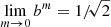 (Paper III). Because
 (A.18)
for all 0 ≤ k ≤ 1, we find immediately that
 (A.19)
where the last transition follows from the fact that the integral is simply equal to unity (Glasser 1976).
Appendix B: Total energy for the most common models
In Table B.1 we list the total energy for some of the most commonly used spherical models. The upper half of the table, above the horizontal line, contains a number of popular one-parameter families of spherical models. The bottom half, below the horizontal line, lists a number of well-known specific models. Each model is completely defined by either the spatial density profile or the surface brightness, and contains the total mass and a length scale (both of which were set to one here) as free parameters.
Total energy for the most commonly used spherical models.
All Tables
Numerical values for the total energy Etot, the gravitational radius rG, the half-mass radius rh, the Spitzer concentration index CS, the TGC concentration index, and the 3D version of the TGC (TGC3D) as a function of m.
All Figures
|
Fig. 1. Dependence of the Spitzer concentration index (Eq. (24)), the TGC index (Eq. (23)), and the 3D TGC index (Eq. (25)) on the Sérsic index m. |
| In the text | |
|
Fig. 2. Location of the Sérsic model family, as well as most other popular spherical toy models, in the (TGC, CS) and the (TGC, TGC3D) planes. The models form banana-shaped trails in the former plane, whereas they are located on an almost perfect one-to-one relation in the latter plane. This shows that the Spitzer concentration index is a poor indicator of the intrinsic 3D concentration, whereas the TGC is a very accurate indicator. |
| In the text | |
Current usage metrics show cumulative count of Article Views (full-text article views including HTML views, PDF and ePub downloads, according to the available data) and Abstracts Views on Vision4Press platform.
Data correspond to usage on the plateform after 2015. The current usage metrics is available 48-96 hours after online publication and is updated daily on week days.
Initial download of the metrics may take a while.