| Issue |
A&A
Volume 630, October 2019
Rosetta mission full comet phase results
|
|
|---|---|---|
| Article Number | A46 | |
| Number of page(s) | 5 | |
| Section | Planets and planetary systems | |
| DOI | https://doi.org/10.1051/0004-6361/201834278 | |
| Published online | 20 September 2019 | |
Revisiting the magnetization of comet 67P/Churyumov-Gerasimenko
1
Institut für Geophysik und extraterrestrische Physik, Technische Universität Braunschweig,
Mendelssohnstr. 3,
38106 Braunschweig, Germany
e-mail: This email address is being protected from spambots. You need JavaScript enabled to view it.
2
Max-Planck-Institut für Sonnensystemforschung,
Justus-von- Liebig-Weg 3,
37077 Göttingen, Germany
Received:
19
September
2018
Accepted:
19
November
2018
Abstract
Context. The landing of the Philae probe as part of the ESA Rosetta mission made it possible to study the magnetization of comet 67P/Churyumov-Gerasimenko (67P) by combining observations from the lander and orbiter. In this work, we revisit the magnetic properties with information gained during the progression of the mission for a comprehensive understanding of the circumstances of Philae’s descent and landing.
Aims. The aim is to derive a limit for any possible magnetization of the cometary material on the surface of 67P. To achieve this, the surface contacts of Philae were analyzed. Combined with a more detailed understanding of the background magnetic field, this allows us to interpret the underlying magnetic measurements in detail.
Methods. We combined magnetic field observations from the ROMAP magnetometer on board Philae with observations from the RPC-MAG instrument on board the Rosetta orbiter. To facilitate this, a correlation analysis was used to correct phase shifts between the observed signals. Additionally, in-flight calibration of the ROMAP offsets was performed using information about the dynamics of Philae during flight. These corrections made it possible to use the orbiter measurements as reference for the comet-based Philae observations. We assumed a simple dipole model and used the magnetic field observations to derive an upper limit for the magnetization of the cometary material.
Results. An upper limit of 0.9 nT for the observed magnetic field on the surface of 67P was derived for any contribution from surface magnetization. For homogeneously magnetized pebbles with a size of typical aggregates in the range of ~5 cm, this translates into an upper limit of ~5 × 10⁻⁵ Am2 kg−1 for the specific magnetic moment. Depending on the exact history of formation, this results in an upper limit of 4 μT for the magnitude of the magnetic field in the solar nebula during the formation of comet 67P.
Key words: magnetic fields / comets: individual: 67P/Churyumov-Gerasimenko
© ESO 2019
1 Introduction
Magnetic field measurements performed during the descent and the four surface contacts of Rosetta’s Philae lander on November 12, 2014 (Glassmeier et al. 2007a; Biele et al. 2015; Ulamec & Taylor 2016), made it possible to derive an upper bound for the magnetization of the target comet 67P/Churyumov-Gerasimenko (67P). The magnetization of comets is not only important because magnetic fields may have played a role in the formation of such objects (Nübold & Glassmeier 1999; Fu & Weiss 2012), but also allows us to constrain the strength of the background magnetic field in the early solar system (Wang et al. 2017). Using concurrent observations from the magnetometer of the Rosetta Plasma Consortium (RPC-MAG, Glassmeier et al. 2007b) and the Rosetta Lander Magnetometer and Plasma Monitor (ROMAP, Auster et al. 2007), Auster et al. (2015) derived an upper limit for the specific magnetic moment of <3.1 × 10⁻⁵ Am2 kg−1 for meter-sized homogeneous boulders. The upper bound for any influence caused by local surface magnetization on the observed magnetic field was chosen to be 2 nT. As the final location of Philae was still unknown, Auster et al. (2015) used an estimated trajectory to reconstruct the distance between the lander and the cometary surface.
After the final landing site of Philae was identified on images (Sierks 2016) taken by the Optical, Spectroscopic and Infrared Remote Imaging System (OSIRIS, Keller et al. 2007), it was possible to further constrain the trajectory of Philae. After the initial touchdown at 15:34:04 UTC (TD1) on November 12, 2014, the lander rebounded, collided with the surface at 16:20:00 UTC (COL), touched down again at 17:25:35 (TD2), and came to a final rest at 17:31:16 UTC (TD3). An analysis of the ROMAP observations also revealed that the magnetometer boom assembly came into contact with the surface material during the second touchdown. As a result, parts of the sensor head were covered with enough surface dust to prevent the ROMAP plasma monitor from detecting any solar wind particles (Heinisch et al. 2017a). The diameter of the ROMAP instrument is approximately 10 cm. The fluxgate magnetometer is located in the middle and the plasma sensors are placed on the outer part of the instrument head. The entrances to the particle detectors at the top and sides of the instrument have a width of approximately 3 cm. Because the dust did not fall off during the remaining flight or alter the deployment angle of the boom, we deduce that the dust aggregates had to be small relative to the size of the sensor. Accordingly, the dust grains blocking the entrances of the sensor had to be smaller than ~3 cm, which is the size of the sensor openings. This is also consistent with particle size distributions estimated by Blum et al. (2017).
Auster et al. (2015) assumed a conservative estimate of the distance between the magnetometer and the surface of 1.2 and 0.4 m, depending on location. While the distances of 1.2 m for the first touchdown and 0.4 m for the collision and final touchdown still apply, a much lower value of 0.05 m (half the sensor head diameter) can be used for the second touchdown as the boom hit the surface. It is therefore possible to resolve much smaller grains in the range of the sensor–surface distance.
The magnetic field observations during descent and landing were dominated by magnetic low-frequency waves that have been studied in detail by Richter et al. (2016) and Heinisch et al. (2017b). These singing comet waves (Richter et al. 2015) with frequencies of 5–50 mHz are created by the interaction between the outgassing comet and the solar wind (Glassmeier 2017). During the descent and rebound, they are the main cause of the variations in the magnetic field, which means that analyzing these waves is a prerequisite when the magnetic observations are to be used to gain insight into the magnetization of the nucleus. The magnetic field measurements also revealed that no magnetic boundary layer exists above the cometary surface, which makes it possible to use the observations of the two RPC-MAG magnetometers in orbit as direct reference for the surface measurements (Heinisch et al. 2016, 2017b). Using these results, we revisit the magnetization of comet 67P.
2 Observations
The ROMAP magnetometer was operating during the entire descent and rebound phase with a constant sampling rate of 1 Hz (Auster et al. 2015). While the RPC-MAG outboard sensor was sampling at a rate of 20 Hz, the inboard sensor measurements are available at a rate of 1 Hz. The RPC-MAG data were processed as described by Richter et al. (2016). To use the RPC-MAG outboard-sensor observations as reference, the measurements were downsampled to 1 Hz to match ROMAP and RPC-MAG inboard observations. While the RPC-MAG inboard sensor was primarily intended for calibration purposes and as possible backup, the measurements can be used for direct scientific analysis as well. As the RPC-MAG sensors are mounted 15 cm apart on a boom that places them only 1.5 m away from the main Rosetta body, spacecraft interference is still present in the observed magnetic field, as explained by Richter et al. (2015). Because of the spatial separation between the IB and OB sensors and the inhomogeneous spacecraft field, the influence on the two sensors is different. Additionally, varying phase shifts (in the range of 2 s) between the Rosetta and Philae measurements were corrected by cross-correlating ROMAP and RPC-MAG signals. The singing comet waves, which were the primary cause for the activity in the magnetic field during the period of interest, were propagating outward from the nucleus with a mean phase velocity of approximately 5.3 km s−1 (Heinisch et al. 2017b). These waves were therefore first observed by ROMAP on the nucleus and later by RPC-MAG in orbit, revealing the related phase shift (Richter et al. 2016; Heinisch et al. 2017b).
2.1 Sensor offsets and lander residual field
As Philae rotated during the entire rebound with a known spin rate (Heinisch et al. 2017a), an in-flight calibration of the sensor-offsets and lander residual field was possible. Residual field effects cannot always be separated from sensor offsets, therefore we use “sensor offsets” for simplicity in the following for the sum of the lander residual field and sensor offset.
With exact knowledge of the offsets, it is possible to determine the calibrated magnitude of the magnetic field, which is independent of the magnetic coordinate system. It follows that with the magnitude, it is possible to relate the ROMAP observations to the RPC-MAG orbiter measurements without introducing errors that are due to attitude uncertainties. Auster et al. (2015) initially assumed constant offsets for all contacts, as the sensor temperature only changed by about ~10° C during the rebound. In general, constant sensor offsets have no direct negative effect on determining the surface magnetization, but they can introduce an additional bias when orbiter and lander measurements are compared. To further reduce uncertainties in the ROMAP observations, the offsets were redetermined individually for the periods before and after each surface contact.
The offsets of the x- and y-components (in the reference frame of the sensor) remained stable for the first part of the rebound. An automatic change from descent to surface operations after the first touchdown caused a change of 1.5 nT in the z-component before the collision as a result of a change in the lander bias field. This change was limited to one component of the magnetic field because of the layout of the relevant electronics. After the collision, the switch-off of the CIVA/ROLIS (Bibring et al. 2007) camera system at 17:21 UTC caused an additional change in bias field in all three components. The derived offsets are summarized in Table 1.
ROMAP offsets in instrument coordinates determined immediately before and after each contact.
2.2 Contact velocities
The velocities for descent and ascent were used to relate the observed magnetic field directly to the height above the surface. Initially, Philae had a descent velocity of −1 m s−1 relative to the comet (Biele et al. 2015; Roll & Witte 2016) and a climb rate of ~0.33 m s−1 after the first touchdown. For the inbound and outbound velocities for the remaining trajectory, the flight reconstruction of Heinisch et al. (2019) was used. This reconstruction is based on a free ballistic flight, with known contact times (Heinisch et al. 2017a), taking into account OSIRIS orbiter camera images of Philae in flight and using the latest SHAP7 digital terrain model (Preusker et al. 2017). The velocities used below are mean values based on the evaluation of several possible trajectories. As the velocity is low relative to the magnetometer sampling rate, errors in the velocity have no significant influence on a possible dipole signature in the magnetic field observations. The descent velocity for the collision that followed after TD1 was approximately −0.33 m s−1, and the lander climbed again with avelocity of ~0.22 m s−1, which was also the descent velocity for the following TD2. Afterward, Philae traveled for an additional ~284 s, which equates to about ~10 m before coming to a final stop at Abydos. During that last flight, Philae reached a maximum height of ~1.5 m above the surface assuming a free ballistic trajectory.
2.3 Magnetic field observations
Any magnetic field created by a magnetized cometary surface should only influence the Philae ROMAP observations and not the RPC-MAG measurements in orbit. Hence, the undisturbed RPC-MAG observations in orbit can be used as reference. Figure 1 shows the magnitude of the magnetic field observed by ROMAP and the RPC-MAG inboard (RPC-IB) and outboard (RPC-OB) magnetometers during descent and ascent of Philae. As Auster et al. (2015) have previously excluded any larger-scale magnetization, the measurements are shown up to a maximum height of 10 m above the surface. The observed field for descent and ascent is displayed for all contacts, except for the flight after TD2 toward TD3 because Philae never exceeded a height of ~1.5 m. For this lastpart, a 200 s interval of magnetic field observations is therefore shown because the exact height above the surface is still uncertain. All three sensors show almost identical signals, with a mean correlation coefficient of ~0.78 between RPC-MAG and ROMAP. As both magnetometers measure almost the same magnetic field, even though RPC is in orbit ~20 km above Philae, there are no significant near-surface effects influencing the magnetic field. Small differences in the magnitude observed in orbit compared to the surface measurements are caused by effects of the near-surface coma.
To further analyze the signals, the difference between the magnitudes of ROMAP and the two RPC-MAG sensors was calculated. This difference signal is shown in Fig. 2 for ROMAP and the RPC-MAG outboard sensor (RPC-OB) as illustration. The descent observations are shown in blue, and the ascent is shown in red. No distance-dependent dipole signature is observable in the difference between the ROMAP and either RPC-MAG inboard or outboard sensor measurements. The standard deviation averaged between the difference between the ROMAP and RPC-MAG IB and OB observations was used to define an upper limit for any possible contribution of surface magnetization to the total observed magnetic field. Because of the uncertainties with the two RPC-MAG sensors, the average of IB and OB was used for the following analysis.
Auster et al. (2015) used the mean value of the averaged absolute values between 10 m and touchdown for descent and ascent to estimate an upper limit of 2 nT for any contribution to the observed field from surface magnetization. As the exact height of Philae during the fight between second and third touchdown is still unknown, this approach can only be used for the first touchdown and collision. For this study the standard deviation of the difference between ROMAP and RPC-MAG was chosen as an estimate for an upper limit. It is not only independent of the specific height above the surface, but also invariant to remaining offsets caused by spacecraft bias fields, which are constant over the entire interval of interest. A height-dependent dipole-like drop-off in the magnetic field potentially caused by surface magnetization would cause additional variance in the observed field, increasing the standard deviation and hence the later derived limit for the magnetization. Additionally, the standard deviation also accounts for the variability of the magnetic field between Philae and Rosetta, which could mask the dipole signature that is caused by small-scale magnetization of the surface. Table 2 shows the standard deviation for the difference between RPC-MAG (averaged over IB and OB) and ROMAP during the ascent and descent. Based on these results, a rounded upper limit of 0.9 nT was chosen for any influence caused by local surface magnetization on the observed magnetic field.
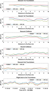 |
Fig. 1 Magnitude of the magnetic field observed by ROMAP (red), RPC-MAG OB (blue), and RPC-MAG IB (green) during the different surface contacts. As the exact height over the surface after second touchdown is unknown, the magnetic field is shown vs. time instead of distance to the surface. |
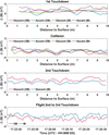 |
Fig. 2 Difference between the magnitudes of the magnetic field observed by ROMAP and the RPC-MAG inboard (IB) and outboard (OB) sensors during descent and ascent of Philae. As the exact height over the surface after second touchdown is unknown, the magnetic field for the climb after second touchdown is shown vs. time instead of distance to the surface. |
Standard deviation between the difference of the RPC-MAG and ROMAP observations for the last 10 m before contact.
3 Magnetization
To determine the magnetic evolution of comet 67P, it was assumed that the measured surface grains were pristine, preserving their initial magnetic properties. While the area around TD1 is covered by a heavily processed fallback-dust layer (Biele et al. 2015), the areas surrounding the collision and TD2 sites are more consolidated (Keller et al. 2015; Thomas et al. 2015; Schröder et al. 2017). We can therefore exclude that the magnetization of the surface material is underestimated because the material is covered with processed dust. With the model proposed by Auster et al. (2015), which is based on randomly oriented, uniformly magnetized cubes with a magnetic dipole moment m, we derived an estimate for the magnetic field B that is caused by a single dipole at the center of the cube:
 (1)
(1)
where r is the spatial vector from the dipole center to the magnetometer, and μ0 is the vacuum permeability. With m = M ⋅ D3, where D is the scale of the cubes or the spatial resolution and M is the magnetization, this becomes
 (2)
(2)
According to the modeling performed by Auster et al. (2015), a single dipole in the second Gaussian orientation (dominating horizontal magnetic moment) can be used to derive a conservative estimate for the magnetization M:
 (3)
(3)
with B = 0.9 nT being the upper limit for the magnetic field and the scalar r = 0.05 m being the closest distance between the material and the sensor (see above). The scale D of the resolvable particles was chosen to be D = 0.05 m, using the closest sensor distance as typical spatial resolution of the measurement. This results in a magnetization of ~3 × 10⁻² A m−1. With a mean density of 533 kg m−3 (Pätzold et al. 2016), this translates into an upper limit for the specific magnetic moment of ~5 × 10⁻⁵ Am2 kg−1 for grains in the range of ~5 cm. The reduction of the spatial resolution to particles with a size of ~5 cm makes it possible to resolve structures in the sub-decimeter size range, which is the characteristic range for cometary agglomerates (Blum et al. 2017) and for the particles the sensor came in contact with, as we described before. Thisis a significant improvement in resolution compared to the more theoretical spatial resolution of D = 1 m that was assumed by Auster et al. (2015) based on the larger distance of sensor to material. Even though the spatial resolution improved by approximately two orders of magnitude, the resulting specific magnetic moment is comparable with what Auster et al. (2015) reported previously: they estimated ~3 × 10⁻⁵ Am2 kg−1. When we assume larger homogeneously magnetized areas on the surface in the range of D ~1 m, as used by Auster et al. (2015), the specific magnetic moment derived based on this analysis decreases by an order of magnitude to ~2 × 10⁻⁶ Am2 kg−1.
4 Discussion and conclusions
Based on a detailed analysis of the measurements of the RPC-MAG and ROMAP magnetometers during the landing and rebound of Philae, it was possible to exclude significant magnetization of the surface of 67P. An upper limit of 0.9 nT for any residual effects caused by surface magnetization was derived. For magnetized pebbles with scales of ~5 cm, which is close to the range of the expected cometary material (Blum et al. 2017), this translates into an upper limit for the specific magnetic moment of ~5 × 10⁻⁵ Am2 kg−1, which is significantly below the initial limit derived by Auster et al. (2015), while simultaneously improving the spatial resolution. When we assume larger homogeneously magnetized boulders in the range of ~1 m, as used by Auster et al. (2015), this results in an upper limit of ~2 × 10⁻⁶ Am2 kg−1. These improvements were possible as a result of the comprehensive understanding of Philae’s descent and rebound trajectory and additional insight into the behavior of the magnetic field that has been gained after the initial study performed by Auster et al. (2015).
Results from the Stardust mission suggest that magnetically susceptible material is present on comets (Ogliore et al. 2010; Berger et al. 2011). Morbidelli & Rickman (2015) suggested that comets like 67P might be collisional remnants of larger objects. In this case, no conclusions can be drawn with regard to the magnetic environment during creation of the comet from the observed magnetization, as collisions would have caused significant reprocessing of the material. If comets are instead primordial rubble piles that experienced negligible thermal or aqueous reprocessing after formation, as described by Davidsson et al. (2016) and Blum (2018), the lack of detectable magnetization might provide insight into the magnetic conditions inside the solar nebula. Two main mechanisms are known to lead to the creation of magnetized particles: accretional detrital remanent magnetization (ADRM), as explained by Fu & Weiss (2012), and accretional attractive remanent magnetization (AARM), as described by Nübold & Glassmeier (2000). Simulations have shown that even in the absence of an external field, AARM can cause the growth of aggregates up to several millimeter in size by the accretion of further magnetic material by single magnetized seed grains (Nübold & Glassmeier 2000). ADRM can create larger coherently magnetized regions (up to decimeter in size) and is based on the alignment of magnetized particles during accretion that is caused by an external magnetic field and can thus play a role either as a stand-alone effect or coupled with AARM. No magnetized regions down to scales of ~5 cm have been detected, which is strong evidence for the absence of ADRM. If comets are largely unaltered primordial rubble piles (Davidsson et al. 2016; Blum 2018), the most likely explanation is the absence of a strong background magnetic field during accretion. This places a threshold on the magnitude of the magnetic field in the solar nebula during the formation of the aggregates the nucleus is made up of. To acquire ADRM, the aligning force of the background magnetic field must overcome other randomizingforces during accretion such as gas drag, Brownian motion, or collisional effects (Fu & Weiss 2012). According to modeling results by Fu et al. (2018) and Biersteker et al. (2018), the magnetic field must have been below ~4 μT for randomizingeffects to overcome the aligning magnetic torque and prevent larger scale magnetization.
Acknowledgements
Rosetta is an ESA mission with contributions from its member states and NASA. We are indebted to the whole Rosetta Mission Team, LCC, SONC, SGS, and RMOC, for their outstanding efforts to make this mission possible. The contributions of the ROMAP and RPC-MAG teams were financially supported by the German Ministerium für Wirtschaft und Energie and the Deutsches Zentrum für Luft- und Raumfahrt under contract 50QP1401. The SPICE kernels used for this work are available as ROS-E/M/A/C-SPICE-6-V1.0 through PSA and PDS.
References
- Auster, H.-U., Apathy, I., Berghofer, G., et al. 2007, Space Sci. Rev., 128, 221 [NASA ADS] [CrossRef] [Google Scholar]
- Auster, H.-U., Apathy, I., Berghofer, G., et al. 2015, Science, 349, aaa5102 [Google Scholar]
- Berger, E. L., Zega, T. J., Keller, L. P., & Lauretta, D. S. 2011, Geochim. Cosmochim. Acta, 75, 3501 [NASA ADS] [CrossRef] [Google Scholar]
- Bibring, J.-P., Lamy, P., Langevin, Y., et al. 2007, Space Sci. Rev., 128, 397 [NASA ADS] [CrossRef] [Google Scholar]
- Biele, J., Ulamec, S., Maibaum, M., et al. 2015, Science, 349, aaa9816 [Google Scholar]
- Biersteker, J. B., Weiss, B. P., Heinisch, P., et al. 2018, Lunar Planet. Sci. Conf., 49, 2642 [NASA ADS] [Google Scholar]
- Blum, J. 2018, Space Sci. Rev., 214, 52 [NASA ADS] [CrossRef] [Google Scholar]
- Blum, J., Gundlach, B., Krause, M., et al. 2017, MNRAS, 469, S755 [CrossRef] [Google Scholar]
- Davidsson, B., Sierks, H., Güttler, C., et al. 2016, A&A, 592, A63 [NASA ADS] [CrossRef] [EDP Sciences] [Google Scholar]
- Fu, R., & Weiss, B. 2012, J. Geophys. Res., 117, E02003 [Google Scholar]
- Fu, R. R., Weiss, B. P., Schrader, D. L., & Johnson, B. C. 2018, Records of Magnetic Fields in the Chondrule Formation Environment, Cambridge Planetary Science (Cambridge: Cambridge University Press), 324 [Google Scholar]
- Glassmeier, K.-H. 2017, Phil. Trans. R. Soc. A, 375, 20160256 [NASA ADS] [CrossRef] [Google Scholar]
- Glassmeier, K.-H., Boehnhardt, H., Koschny, D., Kührt, E., & Richter, I. 2007a, Space Sci. Rev., 128, 1 [NASA ADS] [CrossRef] [Google Scholar]
- Glassmeier, K.-H., Richter, I., Diedrich, A., et al. 2007b, Space Sci. Rev., 128, 649 [NASA ADS] [CrossRef] [Google Scholar]
- Heinisch, P., Auster, H.-U., Richter, I., et al. 2016, Acta Astron., 125, 174 [CrossRef] [Google Scholar]
- Heinisch, P., Auster, H.-U., Plettemeier, D., et al. 2017a, Acta Astron., 140, 509 [NASA ADS] [CrossRef] [Google Scholar]
- Heinisch, P., Auster, H.-U., Richter, I., et al. 2017b, MNRAS, 469, S68 [CrossRef] [Google Scholar]
- Heinisch, P., Auster, H.-U., Gundlach, B., et al. 2019, A&A, 630, A2 (Rosetta 2 SI) [NASA ADS] [CrossRef] [EDP Sciences] [Google Scholar]
- Keller, H. U., Barbieri, C., Lamy, P., et al. 2007, Space Sci. Rev., 128, 433 [NASA ADS] [CrossRef] [Google Scholar]
- Keller, H. U., Mottola, S., Davidsson, B., et al. 2015, A&A, 583, A34 [NASA ADS] [CrossRef] [EDP Sciences] [Google Scholar]
- Morbidelli, A., & Rickman, H. 2015, A&A, 583, A43 [NASA ADS] [CrossRef] [EDP Sciences] [Google Scholar]
- Nübold, H., & Glassmeier, K.-H. 1999, Adv. Space Res., 24, 1163 [NASA ADS] [CrossRef] [Google Scholar]
- Nübold, H., & Glassmeier, K.-H. 2000, Icarus, 144, 149 [NASA ADS] [CrossRef] [Google Scholar]
- Ogliore, R., Butterworth, A., Fakra, S., et al. 2010, Earth Planet. Sci. Lett., 296, 278 [NASA ADS] [CrossRef] [Google Scholar]
- Pätzold, M., Andert, T., Hahn, M., et al. 2016, Nature, 530, 63 [NASA ADS] [CrossRef] [Google Scholar]
- Preusker, F., Scholten, F., Matz, K.-D., et al. 2017, A&A, 607, L1 [NASA ADS] [CrossRef] [EDP Sciences] [Google Scholar]
- Richter, I., Koenders, C., Auster, H.-U., et al. 2015, Ann. Geophys., 33, 1031 [NASA ADS] [CrossRef] [Google Scholar]
- Richter, I., Auster, H.-U., Berghofer, G., et al. 2016, Ann. Geophys., 34, 609 [NASA ADS] [CrossRef] [Google Scholar]
- Roll, R., & Witte, L. 2016, Planet. Space Sci., 125, 12 [NASA ADS] [CrossRef] [Google Scholar]
- Schröder, S., Mottola, S., Arnold, G., et al. 2017, Icarus, 285, 263 [NASA ADS] [CrossRef] [Google Scholar]
- Sierks, H. 2016, ESA ROSETTA Blog, http://blogs.esa.int/rosetta/2016/09/05/philae-found/ [Google Scholar]
- Thomas, N., Davidsson, B., El-Maarry, M. R., et al. 2015, A&A, 583, A17 [NASA ADS] [CrossRef] [EDP Sciences] [Google Scholar]
- Ulamec, S., & Taylor, M. G. 2016, Acta Astron., 125, 1 [CrossRef] [Google Scholar]
- Wang, H., Weiss, B. P., Bai, X.-N., et al. 2017, Science, 355, 623 [NASA ADS] [CrossRef] [Google Scholar]
All Tables
ROMAP offsets in instrument coordinates determined immediately before and after each contact.
Standard deviation between the difference of the RPC-MAG and ROMAP observations for the last 10 m before contact.
All Figures
|
Fig. 1 Magnitude of the magnetic field observed by ROMAP (red), RPC-MAG OB (blue), and RPC-MAG IB (green) during the different surface contacts. As the exact height over the surface after second touchdown is unknown, the magnetic field is shown vs. time instead of distance to the surface. |
| In the text | |
|
Fig. 2 Difference between the magnitudes of the magnetic field observed by ROMAP and the RPC-MAG inboard (IB) and outboard (OB) sensors during descent and ascent of Philae. As the exact height over the surface after second touchdown is unknown, the magnetic field for the climb after second touchdown is shown vs. time instead of distance to the surface. |
| In the text | |
Current usage metrics show cumulative count of Article Views (full-text article views including HTML views, PDF and ePub downloads, according to the available data) and Abstracts Views on Vision4Press platform.
Data correspond to usage on the plateform after 2015. The current usage metrics is available 48-96 hours after online publication and is updated daily on week days.
Initial download of the metrics may take a while.