| Issue |
A&A
Volume 627, July 2019
|
|
|---|---|---|
| Article Number | A75 | |
| Number of page(s) | 15 | |
| Section | Interstellar and circumstellar matter | |
| DOI | https://doi.org/10.1051/0004-6361/201935528 | |
| Published online | 03 July 2019 | |
The environment of supernova remnant VRO 42.05.01 as probed with IRAM 30m molecular line observations★
1
Anton Pannekoek Institute for Astronomy, University of Amsterdam,
Science Park 904,
1098
XH Amsterdam, The Netherlands
e-mail: M.AriasdeSaavedraBenitez@uva.nl
2
GRAPPA, University of Amsterdam,
Science Park 904,
1098
XH Amsterdam, The Netherlands
3
SRON, Netherlands Institute for Space Research,
Utrech, The Netherlands
Received:
24
March
2019
Accepted:
6
June
2019
Context. The environment of supernova remnants (SNRs) is a key factor in their evolution, particularly at later stages of their existence. Mixed-morphology (MM) SNRs have a peculiar centre-filled X-ray shape that remains enigmatic. It is often assumed that they evolve in very dense environments, and that the X-ray morphology is due to interactions between the SNRs and their surroundings.
Aims. We aim to determine whether VRO 42.05.01 is embedded in, and interacting with, a dense molecular environment. We also aim to understand the multi-wavelength emission from the environment of this SNR, and whether the interstellar material can be responsible for the the MM nature of the source, and for its strange radio and optical shape.
Methods. We used the IRAM telescope in Pico Veleta, Spain, to search for signs of interaction between the SNR and neighbouring molecular clouds. We observed a region of 26′ × 14′ towards the west of VRO 42.05.01 and a region of 8′ × 4′ towards the north of the remnant in the 12CO J = 1−0, 13CO J = 1−0, and 12CO J = 2−1 transitions with the EMIR receiver. We made maps of the properties of the observed molecular clouds (peak temperatures, central velocities, velocity dispersions), as well as maps of column density along the line of sight, and ratio of the 12CO J = 2−1 to 12CO J = 1−0 transitions. We also analyse archival optical, infrared, and radio spectroscopic data for other hints on the nature of the medium.
Results. We do not find conclusive physical proof that the SNR is interacting with the few, clumpy molecular clouds that surround it in the region of our observations, although there is some suggestion of such interaction (in a region outside our map) from infrared emission. We find that there is a velocity gradient in one of the molecular clouds that is consistent with a stellar wind blown by a 12−14 M⊙ progenitor star. We reassess the literature distance to VRO 42.05.01, and propose that it has a local standard of rest velocity of − 6 km s−1, and that it is located 1.0 ± 0.4 kpc away (the earlier distance value was 4.5 ± 1.5 kpc). We find that a dust sheet intersects VRO 42.05.01 and is possibly related to its double shell-shaped morphology.
Key words: ISM: supernova remnants / ISM: clouds / ISM: molecules / ISM: general
The reduced data cubes for all molecular observations are only available at the CDS via anonymous ftp to cdsarc.u-strasbg.fr (130.79.128.5) or via http://cdsarc.u-strasbg.fr/viz-bin/qcat?J/A+A/627/A75
© ESO 2019
1 Introduction
Core-collapse supernova explosions often occur near massive molecular clouds (MCs), the sites of stellar birth. Moreover, massive stars affect their environment through radiation and winds. The complex environment in which a star dies can have a profound effect on the evolution of its supernova remnant (SNR). The effect is of particular importance at late times, when the remnant has swept up many times over the mass of its progenitor, and the original imprint of the explosion is lost.
There are several ways to establish interaction between a SNR and neighbouring MCs (Jiang et al. 2010); a common one is through molecular observations of CO at different transitions and isotopes (e.g. Huang & Thaddeus 1986). In this work we present new molecular observations in the direction of SNR VRO 42.05.01 (G 166.0 +4.3), a peculiarly shaped mixed-morphology (MM) SNR in the direction of the Galactic anti-centre.
Mixed-morphology supernova remnants (Rho & Petre 1998) are a class of supernova remnants that display a shell-shape in the radio, but are centre-filled in the X-rays. The X-ray emission is thermal in nature and not caused by a pulsar wind. These sources tend to be associated with the denser parts of the interstellar medium (ISM), and are more likely to be interacting with nearby MCs than SNRs are in general (see Table 4 in Vink 2012). There is no consensus in the field over what the mechanism is by which SNRs become MM SNRs, but the two main models (White & Long 1991; Cox et al. 1999) invoke a dense environment in which the SNR evolves. According to the former, there are dense clouds nearby the explosion site that survive the shock passage, are evaporating inside the hot interior of the SNR, and are responsible for the X-ray emission. The latter attributes the difference in radio and X-ray morphology to the interaction of the shock with a dense ISM: as the shock becomes radiative, the shell will no longer emit X-rays. In addition to these there are other models, such as the reflected shock model (Chen et al. 2008), which attributes the MM to a dense wall that reflects the forward shock back into the direction of the ejecta, or the conduction phase model (Kawasaki et al. 2005), which suggests that the MM is a stage in the life of all SNRs.
VRO 42.05.01 (Fig. 1) is a relatively well-studied SNR with a puzzling shape. It is formed by two structures that intersect in a sharp line: the semicircular, smaller “shell”, and the triangular “wing” (see Fig. 1). It has been studied in the X-rays (Burrows & Guo 1994; Guo & Burrows 1997; Bocchino et al. 2009; Matsumura et al. 2017), in the optical (van den Bergh et al. 1973; Fesen et al. 1985; Boumis et al. 2016), in the radio continuum (Landecker et al. 1982; Pineault et al. 1985; Leahy & Tian 2005; Arias et al. 2019), and in H I (Landecker et al. 1989). It has also been detected in GeV γ-rays (Araya 2013), although this detection could be due to a chance alignment with an extragalactic source.
For a source with as unusual a morphology as VRO 42.05.01, it is natural to think that the environment must have had a significant role in its evolution. The most comprehensive model of the source to date is that of Pineault et al. (1987), who proposed that the supernova occurred in a warm medium of intermediate density (which surrounds the shell) and that a part of the remnant (the wing) broke out into a diffuse interstellar cavity, possibly blown by a stellar wind or one or more earlier SNRs. In Arias et al. (2019) we elaborated on this model, suggesting that the sharp triangular cavity of the wing could be due to the progenitor star exploding as it was moving supersonically into the more rarefied medium, forming a bow shock whose structure remains visible in the SNR.
Our aim in this paper is to understand the environment of VRO 42.05.01 and how it has affected the remnant’s morphology. How a particular remnant developed its shape is anecdotal; we are more generally trying to understand the process by which this remnant became of mixed-morphology, and the role of its medium in confining the X-ray emitting material in the interior of the radio shell.
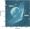 |
Fig. 1 VRO 42.05.01 at 1420 MHz. This map taken from the CGPS. Labelled are the regions referred to throughout the text as “shell” (the small semicircle) and “wing” (the large triangle). We note that a sharp boundary separates the two regions. |
2 Data
2.1 IRAM 30m observations
We performed 3 and 1 mm heterodyne observations toward the western side of VRO 42.05.01 with the IRAM 30m telescope, over several days in the summer and fall of 2018 (3, 4, and 5 July, and 24, 25, and 26 October) under project 045-18 (PI, María Arias). The observations amounted to approximately 23 hours on-source, with varying weather and elevation conditions, resulting in uneven noise levels in our map.
We simultaneously mapped 12CO J = 1−0 (at 115.271 GHz), 13CO J = 1−0 (at 110.201 GHz), and 12CO J = 2−1 (at 230.540 GHz) emission toward VRO 42.05.01 and its vicinity, in the on-the-fly mode with the Eight MIxer Receiver (EMIR). The fast Fourier transform spectrometers (FTSs) were tuned to the 200 kHz resolution, which provided a velocity resolution of 0.25 km s−1 for the 12CO J = 2−1 line, and 0.5 km s−1 for the 12CO J = 1−0 line. The beam efficiencies were 0.78 and 0.58 for the J = 1 − 0, and J = 2−1 transitions, respectively.
The data were then converted to 12CO J = 1−0, 12CO J = 2−1, and 13CO J = 1−0 main beam temperature (Tmb) cubes with a grid spacing of 11.75′′ and a velocity resolution of 0.5 km s−1. The final map has 300 channels, spanning the velocity range from − 99.5 to + 50 km s−1. The data were reduced with the GILDAS/CLASS package1.
The molecular data in Tmb (K) for the 12CO J = 1−0 transition are plotted in Figs. 2 and 3. The molecular data for the 12CO J = 2−1 and 13CO J = 1−0 transitions are plotted in the appendix (Figs. A.2–A.4). Finally, the rms noise for each transition, for each pixel, is also in the appendix (Fig. A.1).
2.2 Other archival data used for this work
In this paper, we tried to put our IRAM molecular observations in a multi-wavelength context to best understand the environment of VRO 42.05.01. We used the 1420 MHz continuum maps from the Canadian Galactic Plane Suvey (CGPS, Taylor et al. 2003) to show the regions of synchrotron emission. We also used the 21 cm data cubes from the CGPS to study the neutral hydrogen distribution around the remnant. In the infrared we used data from the Wide-Field Infrared Survey Explorer all-sky survey (WISE; Wright et al. 2010), at wavelengths of 3.4, 4.6, 12, and 22 μm. Finally, we took the optical Hα and [S II] maps from the Middlebury Emission-Line Atlas of Galactic SNRs2 (Winkler et al., in prep.). The optical images were taken with the 0.9 m KP Schmidt telescope at the Kitt Peak National Observatory between January 15 and 19, 1996. The Hα filter had a central wavelength of 6560.9 Å and a width of 25.3 Å, and the [S II] filter was centred at 6718.3 Å and was 47.9 Å wide.
3 Results
In the region of our observations, for all three CO lines, there are two velocity ranges where emission is present. Between roughly − 28 and − 12 km s−1 (which we refer to as the distant component) different structures appear and fade continuously within the range, and, after a few dark channels, the emission begins to reappear in the range of − 8 to − 1 km s−1 (which we refer to as the close component). The remaining velocity ranges included in our observations show only noise.
3.1 Method
We first aimed to determine some of the basic parameters of the molecular clouds observed in our data. In order to measure the peak temperature(T0), velocity spread (Δv), and central velocity of the emission components, we fitted each pixel in the data cube to two gaussians, one restricted to the velocity range of the distant component, and one restricted to the range of the close component. For each Gaussian the fit produceda height (peak temperature), full-width at half-maximum (velocity spread), and centre (velocity of the peak). A sample of what the fit did for each pixel is shown in Fig. 4. The results for the 12CO transitions are plotted in Fig. 5.
3.2 Ratio maps
Ambient molecular clouds have a temperature of ~10 K, typical in the ISM. For 10 K, the ratio of 12CO J = 2−1 and 12CO J = 1−0 is smaller than one. In shock-heated gas, the temperature rises to T ≫ 10 K, which causes the 12CO J = 2−1 and 12CO J = 1−0 ratio to become larger than one (provided that the lines are optically thin), or approximately one (in the optically thick case). For this reason, the ratio of 12CO J =2−1 to 12CO J = 1−0 is commonly used as an indicator of the presence of shocks in a molecular cloud (Seta et al. 1998).
For the pixels where the 12CO J =2−1 and 12CO J =1−0 best-fit velocities of the peaks matched, and for which the best-fit peak temperature was more than five times above the rms noise for that pixel (Fig. A.1), we took the ratio of the peak temperatures. These are plotted in the top-right panels of Fig. 5. All the values are below one, which indicates that these are ambient molecular clouds that have not been heated by the SNR shock.
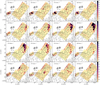 |
Fig. 2 Tmb (K) for the 12CO J = 1− 0 transition for the distant molecular cloud components, corresponding to velocities between − 27.5 and − 15.0 km s−1. Overlaid arethe radio contours at 1420 MHz in units of brightness temperature at 4.8, 5.0, 5.5, and 6.0 K. The velocities are indicated in the upper left corner of each panel. All figures in the same row share the same colour bar, plotted at the left end of each row. |
3.3 Column density maps
It is possible to estimate physical parameters such as optical depth and molecular column density from the 13CO J = 1−0 measurements, provided that the rotational levels of the 13CO molecule are in local thermodynamic equilibrium (LTE).
In practical units, the optical depth and column density of 13CO are (Kawamura et al. 1998):
![\begin{equation*} \tau_0^{13} = - \ln \left[1 - \frac{T_0^{13}}{\frac{5.29}{e^{5.29/T_{\mathrm{ex}}}-1}-0.87} \right], \end{equation*}](/articles/aa/full_html/2019/07/aa35528-19/aa35528-19-eq1.png) (1)
(1)
![\begin{equation*} \left[\frac{N^{13}}{\mathrm{cm}^{-2}}\right] = 2.42\,{\times}\,10^{14} \left(\frac{\Delta v}{\mathrm{km\,s}^{-1}} \right) \left(\frac{T_{\mathrm{ex}}}{\mathrm{K}}\right) \frac{\tau_0^{13}}{1 - e^{-5.29/T_{\mathrm{ex}}}}.\end{equation*}](/articles/aa/full_html/2019/07/aa35528-19/aa35528-19-eq2.png)
![\begin{equation*} T_0^{13} = \left[J^{13}(T_{\mathrm{ex}}) - J^{13}(T_{\mathrm{bg}})\right] \left(1 - e^{-\tau_0^{13}}\right), \end{equation*}](/articles/aa/full_html/2019/07/aa35528-19/aa35528-19-eq3.png)
where Tex is the excitation temperature of the J = 1−0 transition of12CO in K (the same asfor 13CO), Tbg = 2.7 K, and J(T) = 1 ∕ (exp[−5.29∕T] − 1).
We took the excitation temperature of the J = 1−0 transition of12CO to be Tex = 10 K. We cannot calculate the excitation temperature directly from our measurements because we would need to assume that the J = 1−0 transition of 12CO is optically thick everywhere (this assumption can break down at the edge of the clould, which could fall within our pixel) and also that the filling factor f is 1. The low Tmb temperatures we measured (see Figs. 2 and 3) suggest that the molecular cloud might be composed of clumps smaller than the telescope beam (f < 1).
Using Eq. (2), Tex = 10 K, a N(H2) to N(CO) ratio of 5 × 10⁵ (Dickman 1978), and assuming that the 13CO is in LTE, we obtained the maps in Fig. 6. Due to the uneven noise levels in our map (clearly visible in the rms plots in Fig. A.1), we present the regions where we have a 3σ detection of the hydrogen column density and those for which we only have an upper limit separately.
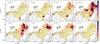 |
Fig. 3 Tmb (K) for the 12CO J = 1− 0 transition for the close molecular cloud components, corresponding to velocities between − 8.5 and − 1.0 km s−1. Overlaid arethe radio contours at 1420 MHz in units of brightness temperature at 4.8, 5.0, 5.5, and 6.0 K. The velocities are indicated in the upper left corner of each panel. All figures in the same row share the same colour bar, plotted at the left end of each row. |
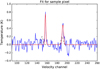 |
Fig. 4 Example of the fit that produces Fig. 5 for a single pixel. The data points from the cube are plotted in blue, the initial guess for the fit in dashed black, and the fit result is in red. The x-axis is in units of the cube velocity channels, where channel 200 corresponds to 0 km s−1, and channelsare 0.5 km s−1 apart. For this pixel the peaks are 0.785 K at − 21.6 km s−1 (channel 156.7), and at 0.508 K at − 4.2 km s−1 (channel 191.5). |
3.4 Position-velocity maps for possible wind component
One can see from the plot of best-fit central velocity of the close component (Fig. 5, lower-left corner) that there is a velocity gradient from the position RA = 5:25:50, Dec = +43:00:34 that goes north-west, at an angle of 72o with the horizontal.
Later in this paper we argue that this gradient is a result of the interaction between a stellar wind and the molecular cloud. In Fig. 7 we present a position-velocity diagram of a slice taken along the line that goes from RA = 5:25:50, Dec = +43:00:34 to RA = 5:25:09, Dec = +43:25:36, forming a 72° angle with the horizontal, as indicated by the blue line in Fig. 5 lower-left map.
It is clear from the position-velocity diagram that there is a part of the cloud (near RA = 5:25:50, Dec = +43:00:34) that is moving differently from the quiescent velocity of the system of − 4.5 km s−1. The measured velocity difference is of 4.5 km s−1 in the blue-shifted direction, although the real velocity difference could be larger, since this feature is visible in the edge of our map. One can see in the top four maps of Fig. 3 that this disturbed component begins to appear in the southern edge of our map and moves north-west.
4 The molecular environment of VRO 42.05.01
4.1 A clumpy molecular medium and a diffuse environment
The channel maps show that the molecular gas near VRO 42.05.01 is very clumpy. The 12CO J =1−0 emission has a main beam temperature Tmb ≲ 7 K for the vast majority of pixels (see Fig. 5, and channel maps in Figs. 2 and 3), cooler than the ~10 K typical of ISM molecular clouds. This points to the presence of unresolved clumps, of angular size smaller than the telescope beam (θclump < 0.11 pc for a distance of 1 kpc, for the close component; θclump < 0.68 pc for a distance of 6 kpc, for the distant component).
Another important aspect to note is that the SNR is in an environment with a low molecular column density (see 3σ measurements and upper limits in the  distribution in Fig. 5). Our measured column densities are as high as 1.7 × 1021 cm−2 for only three small (~1′) regions in the face of the SNR, and for most of the remnant we measure an upper limit of 3.1 × 1020 cm−2 or lower. These values are smaller than earlier X-ray measurements in Guo & Burrows (1997), who found ~ 2.9 × 1021 cm−2 for regions of 11′ × 11′, although their X-ray observations and our IRAM observations do not overlap. Moreover, the X-ray measurement of column density is sensitive to neutral and ionised hydrogen, in addition to molecular hydrogen, so it is not surprising that the column density measured here is smaller.
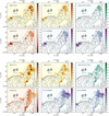 |
Fig. 5 Results from fitting the distant (top) and close (bottom) components of the line profile to a Gaussian. For each of the two panels: height of the 12CO J = 1− 0 line in K (top, left), height of the 12CO J = 2− 1 line in K (top, middle), full-width at half maximum of the 12CO J = 1− 0 line in km s−1 (bottom, middle), full-width at half maximum of the 12CO J = 2− 1 line km s−1 (bottom, right), and best-fit central velocity in km s−1 (bottom, left). For regions with signal over 5σ, the ratio of 12CO J = 2− 1 to 12CO J = 1− 0 is plotted inthe top, right. Overlaid are the radio contours at 1420 MHz in units of brightness temperature at 4.8, 5.0, 5.5, and 6.0 K. Note the velocity gradient from the south to the north-west in the best-fit central velocity of the close component plot (lower left corner). The line used to make the position-velocity plot in Fig. 7 is indicated in this map in dark blue. |
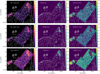 |
Fig. 6 From left to right, log of the optical depth of 13CO ( |

 |
Fig. 7 Position-velocity plot for a line that goes from RA = 5:25:50, Dec = +43:00:34 to RA = 5:25:09, Dec = +43:25:36 with a 72o inclination (see Fig. 5, lower-left corner) along the large velocity gradient seen at velocities of − 8 to − 2 km s−1. |
4.2 There is no physical proof of interaction between the supernova remnant shock and the molecular clouds in the region of our observations
In our observations, we do not find any conclusive physical proof that the SNR shock has reached its neighbouring molecular clouds. For the most part, we do not find broadened or asymmetric lines (see Fig. 5, in blue, for best-fit line widths), norhigh ratios between lines of different excitation states (Fig. 5, in green). The blue maps in Fig. 5 (the bottom ones, of the close component) do show a region towards the west where the line widths are > 4 km s−1. Upon examination, these broad lines turn out to be an artefact of our fitting routine (see Fig. 8). There are two clumps along the line-of-sight of these pixels, which the fitting routine tried to fit as one single Gaussian in this velocity range, resulting in a wider FWHM and a shorter height. When we corrected by adding a second Gaussian component, the two clumps were fitted by Gaussians with narrow FWHM (1.62 km s−1), again indicating an unperturbed medium.
At an even more basic level, there are no obvious morphological coincidences between the supernova remnant and the molecular cloud, in the form of indentations or borders where these two structures encircle each other. The molecular cloud features that we see are on the face of the remnant, where the radio and optical emission are relatively faint (although this is likely because we are looking at the shock front edge-on and hence there is no limb-brightening, and not because there is no shock there).
We cannot say, from the IRAM observations, that the supernova remnant shock has reached and heated its surrounding molecular cloud in the 26′ × 14′ region towards the west and the 8′ × 4′ region towards the north of VRO 42.05.01 that we observed. The environment appears to be relatively empty of molecular clouds, we do not detect any sharp density gradients in the face of the remnant separating shell and wing, and, at least in the region of our observations, it is not likely that dense molecular gas is responsible for the strange shape of this source.
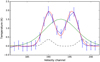 |
Fig. 8 Averaged spectrum for the values in Fig. 5, blue plots, where the FWHM of the lines are greater than 3.5 km s−1. The fitting routine did not account for two clumps along the line-of-sight of a pixel for this range in velocities, and so tried to fit the two components as a single Gaussian with a broad FWHM (in green, corresponding to a FWHM of 4.4 km s−1). When we allowed for a second Gaussian term to be added to the model, the two clumps are fitted by Gaussians with narrow FWHM (1.62 km s−1). The data points from the cube are plotted in blue, the initial guess for the fit in dashed black, and the fit result is in red. The x-axis is in units of the cube velocity channels, where channel 200 corresponds to 0 km s−1, and channelsare 0.5 km s−1 apart. |
4.3 Wind parameters
We can veryroughly estimate some properties of the stellar wind from the expanding bubble revealed in our observations (Fig. 7).
The detection of the velocity gradient is limited to a small region in the southernmost corner of our map. In fact, the region with a gradient appears to coincide with some features that follow the semicircle of the small shell. The rim of the shell is more easily visible in the optical, as one can see in Fig. 9. Although the feature is, unfortunately, at the edge of our map, it seems to follow the Hα morphology. For this reason we took the radius ofthe wind R to be the radius of the shell (which subtends an angle of 29′), 8.4 pc at a distance of 1 kpc.
Combining Eqs. (51) and (52) in Weaver et al. (1977), which describe the evolution of an interstellar bubble, we arrived to:
 (4)
(4)
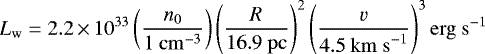
where Lw is the luminosity of the stellar wind, v is the expansion velocity of the shell (the difference between the velocity of the molecular cloud and the disturbed component, as one can see in Fig. 7; we take v = 4.5 km s−1, although this is a lower limit), n0 is the number density of hydrogen atoms, and R is the radius of the bubble. Pineault et al. (1987) propose that the density of the medium that surrounds the SNR could be 1 cm−3. We use this density value for our mass-loss estimate, but keep the dependency on n0 explicit.
The wind luminosity is related to the mass-loss rate of the star as:
 (5)
(5)
where vw is the wind velocity and Ṁ is the mass-loss rate of the star due to the wind.
A luminosity Lw = 2.2 n0 × 1033 erg s−1, and a wind velocity of 1000 km s−1 corresponds to a mass-loss rate of 7.7 n0 × 10−9 M⊙ yr−1, over a period of 1.1 × 10⁶ yr. These are reasonable parameters for the main-sequence wind of a star of 12− 14 M⊙ (Chen et al. 2013), which could be the progenitor of VRO 42.05.01.
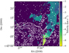 |
Fig. 9 Best-fit central velocity for the close component (same as Fig. 5, lower left). Overlaid are the contours of VRO 42.05.01 in Hα at (5, 10, 20) × 10−17 ergs cm−2 s−1. It should be noted that the velocity gradient (which fades from yellow to green) appears to follow the semicircle (bright in Hα, and also in radio synchrotron) of the small shell of VRO 42.05.01. |
4.4 Geometry of the system
Landecker et al. (1989) first studied the neutral hydrogen environment of VRO 42.05.01. They identified a series of features that seemed to indicate that the SNR was interacting with a surrounding H I structure at a systemic velocity of − 34 km s−1. In particular, they found a cavity in the H I distribution at − 28 km s−1, which, they proposed, is an interstellar cavity in which the remnant is located. Due to the large errors in kinematic distances in the direction of the Galactic anti-centre, they could only estimate that the distance to the cavity (and, hence, the remnant) should be the distance of the Perseus arm, which they take to be 4.5 ± 1.5 kpc.
In our earlier work on VRO 42.05.01 (Arias et al. 2019), we followed this claim up by examining the H I cubes from the CGPS (Taylor et al. 2003). We did not see some of the purported features of interaction listed in Landecker et al. (1989), including the alleged H I cavity. Initially we were inclined to believe that the systemic velocity of VRO 42.05.01 was − 28 km s−1, that of the cavity, or otherwise close to the velocity of the H I structure that Landecker et al. (1989) associated with the remnant, − 34 km s−1, but the observed distribution in molecular gas points to the remnant being significantly closer.
To convert velocities to distances, we used the rotation curve of the outer Galaxy in Reid et al. (2014, plotted for the coordinates of VRO 42.05.01 in Fig. 10). According to this curve, the component we refer to as “close” is located between 0.35 and 1.35 kpc from the Sun, and the “distant” component is between 2.25 and 8 kpc away. From the central velocity plots (Fig. 5, in red) we see that the bulk of central velocities in the close component are approximately − 4 km s−1, and for the distant component, − 20 km s−1. This corresponds to 65 ± 5 pc and 4.6 ± 0.5 kpc, respectively. We expect the SNR to be further away than − 4 km s−1, since the region with a velocity gradient has not been shocked, but close enough to that velocity that its progenitor could blow the wind bubble that caused the gradient. This suggests that VRO 42.05.01 has a local standard of rest velocity of approximately − 6 km s−1, corresponding to a distance of 1.0 ± 0.4 kpc. We note, however, that the flat rotation curve does not always apply to the Perseus arm (e.g. Roberts 1972; Foster & Brunt 2015), and so these distance estimates should be taken with a grain of salt.
If the blue-shifted velocity gradient observed in Fig. 7 is indeed due to a wind blown by the progenitor star of the remnant, then the remnant should be behind the cloud. It should be far enough from the cloud that the remnant shock front has not yet reached and heated the molecular cloud (as evidenced from the 12CO J = 2−1 to 12CO J = 1−0 ratio, Fig. 5), but still close enough that the companion wind could have reached and disrupted the molecular gas. Due to the large distance (>1 kpc) between the close and distant molecular components, according to our interpretation, the supernova remnant and the distant velocity component are unrelated. This distant component is probably associated with the Perseus arm.
If VRO 42.05.01 was indeed 4.5 kpc away, at a Galactic latitude of 4.3o, this would correspond to 340 pc above the Galactic plane, and the physical size of the remnant in its longer direction (45′) would be 59 pc. The height above the plane is slightly problematic if VRO 42.05.01 is the remnant of a core-collapse explosion, because the scale height of the Milky Way thin disk (where massive stars typically reside) is ~300 pc (Jurić et al. 2008), and for OB associations the scale height is only ~40 pc (Bobylev & Bajkova 2016). If, as we suggest, the distance to the remnant is ~1 kpc, its height above the Galactic Plane would be 75 pc, and its angular size would correspond to 13 pc.
According to our line of reasoning, we have the following scenario: the supernova remnant is outside the edge of the close molecular cloud (~1 kpc away). The stellar wind has had to blow a cavity larger than the shock front of the remnant, at least in the direction of the molecular cloud (for the shell). For our rough estimate of the luminosity of the wind and mass-loss rate of the progenitor we took the radius of the bubble to be the radius of the small shell. In fact, the radius of the small shell delimits the shock front; if the remnant is right at the edge of the close molecular cloud, the stellar wind would have had to blow a cavity slightly larger than 8.4 pc.
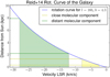 |
Fig. 10 Distance from the Sun as a function of measured local standard of rest velocity as per Reid et al. (2014). The distant molecular component corresponds to distances between 2.25 and 8 kpc, and the close component corresponds to distances between 0.35 and 1.35 kpc. |
5 The dust and H I environment of VRO 42.05.01
5.1 An H I cavity at −6 km s−−1
In light of our new suggested distance for VRO 42.05.01, we revisited the H I cubes from the CGPS for features at velocities closer than those around the range of − 22 to − 54 km s−1studied by Landecker et al. (1989), and that we followed up on in Arias et al. (2019). The H I environment at the velocity ranges around our alleged systemic velocity for VRO 41.05.01, − 6 km s−1, is quite crowded. The most suggestive features we found in the CGPS cube are a cavity with roughly the shape of the SNR, which can be seen in Fig. 11 at − 6.4 km s−1, and an H I bright region just north of the remnant, in the shell region (which has traditionally been thought to be in a dense environment). However, the H I data shows a lot of structure, and coincidental similarities between the remnant and H I features are possible.A detailed study of the H I features at these velocities, such as the one done by Landecker et al. (1989), is beyond the scope of this paper, but for completeness we wanted to note that the H I data is not at odds with our suggested value for the systemic velocity as derived from the CO observations.
The H I bright region near the shell, north of the remnant (seen most clearly in Fig. 11, second panel, at − 6.4 km s−1) also coincides with a very bright radio and optical spot in VRO 42.05.01’s small shell. In Arias et al. (2019) we note that this region has aradio spectral index that steepens at low frequencies, which we argue is a result of the properties of high compression ratio shocks, and requires a high post-shock density. If related, this bright H I feature could be responsible for the bright radio and optical emission, as well as support our proposed explanation for low-frequency steepening.
5.2 Hints from the infrared and the optical
The infrared is an important regime for understanding the Galactic environment. In particular, infrared emission can be a diagnostic of interaction of a SNR with relatively dense gas, since shocked gas cools through line emission, and many important cooling linesoccur in this part of the spectrum (Reach et al. 2006).
In Fig. 12 we display maps of VRO 42.05.01 at 3.4, 4.6, 12, and 22 μm from the WISE survey (Wright et al. 2010), as well as the Hα and [S II] maps from the Middlebury Emission-Line Atlas of Galactic SNRs (Winkler et al., in prep.). We note the following features (labelled for clarity in Fig. 13):
- 1.
The 12 and 22 μm maps show a broad band of emission that goes from the south-east corner of the map, along the line separating the shell and the wing, and that seems to encircle the shell, continuing the morphology from the stellar wind we found in the IRAM molecular data, and that goes on to follow the boundary between shell and wing to the north-western corner of the map.This feature is external to the remnant, and part of a large structure seen more clearly in Fig. 13 (labelled in blue). In the region of our IRAM observations, this is the only structure that could conceivably be interacting with the SNR. It could be the boundary of the density discontinuity invoked by models to explain the source. We find it is the most likely candidate to be responsible for the unusual shape of this SNR in the area covered by our IRAM observations.
- 2.
There is a filament in the wing, to the west of the remnant, that goes from north to south, that matches a bright radio synchrotron feature (labelled in red in Fig. 13). This feature is visible in all the infrared bands, although it is very faint by 3.4 μm. It is alsovisible in the optical maps.
- 3.
There are a series of filaments internal to the wing, seen at 4.6 and 12 μm, that have very faint radio and optical counterparts. These filaments broadly trace a semicircle that continues the semicircle of the small shell.
Reach et al. (2006) note that infrared emission from SNRs can be due to synchrotron emission, shock-heated dust, atomic fine-structure lines, and molecular lines, but that it is challenging to disentangle the contribution of each component from colour maps.
Infrared synchrotron emission from SNRs requires a high radio luminosity, and VRO 42.05.01 is a relatively faint object (7 Jy at 1 GHz for an angular size of 45′ × 80′) although with a flat radio spectral index, α ≈ 0.37 (Leahy & Tian 2005). The only feature that coincides with a radio-bright filament is feature 2. However, the filament appears to be brighter at 12 μm than at 22 μm, which points to a different emission mechanism than synchrotron.
Features 2 and 3 are similar in that they are filamentary, and likely associated with the radiative SNR shocks. The main difference between them is that feature 2 coincides with radio- and optical-bright filaments, which clearly trace the SNR shock, whereas the radio and optical emission associated with the filaments that compose feature 3 are very faint. Infrared atomic fine-structure lines, and vibrational lines from molecules are expected in radiative shocks: the dense gas quickly cools to temperatures of 100−1000 K and infrared transitions are excited (Reach & Rho 2000). There are a number of forbidden emission lines that fall within the WISE bandpasses: most notably, the S(3) and S(9) lines of molecular hydrogen (9.666 and 4.695 μm) fall within the 12 μm and the 4.6 μm WISE bands. These lines have been detected in other MM SNRs (W28, W44, 3C391; Reach & Rho 2000).
The filaments that form feature 2 seem to radiate in the 3.4, 4.6, and 12 μm bands, although not in the 22 μm. It is not possible to disentangle what elements or molecules are radiating in these bands without spectroscopic data. In the case of the filaments that compose feature 3, we suspect that the emission is due to molecular hydrogen, since it is visible at 4.6 and 12 μm, but not at 3.4 and 22 μm. Feature 2 could also be due to interaction with molecular hydrogen, and the coincident 3.4 μm emission could be shocked dust. This would signal interaction between the supernova remnant shock and a nearby molecular cloud; targeted molecular line observations towards this region could confirm this hypothesis. Projection effects might be responsible for the faint radio synchrotron at the location of the filaments. A further point to note is that the feature 3 filaments coincide with the peak in X-ray brightness as seen in Fig. 4 of Bocchino et al. (2009) and Fig. 1 of Matsumura et al. (2017).
Feature 1 is part of a large sheet of dust that cuts through the remnant. Its coincidence with the flat line that separates the shell and the wing, as well as its wrapping around the shell are very suggestive that this structure has had a role in producing the two-shell shape of this source. It is the only structure that we have found that has such a clear morphological similarity with the SNR at large scales.
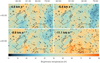 |
Fig. 11 Velocity distribution of HI emission towards VRO 42.05.01 at the range of velocities that corresponds to the close molecular cloud. The data cube was taken from the CGPS. Overlaid are the radio contours at 1420 MHz in units of brightness temperature at 2.5, 3.7, 4.8, and 6 K. The wedges in the upper left corner of each plot correspond to the velocity of each slice. The brightness temperature TB colour scale is the same for all plots. |
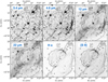 |
Fig. 12 3.4, 4.6, 12, and 22 μm (WISE, Wright et al. 2010), Hα and [S II] (Middlebury Emission-Line Atlas of Galactic SNRs, Winkler et al., in prep.) maps of VRO 42.05.01. Overlaid are the radio contours at 1420 MHz in units of brightness temperature at 4.8 and 6.0 K. |
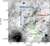 |
Fig. 13 12 μm WISE map with 1420 MHz radio contours in units of brightness temperature at 4.8 and 6.0 K. Labelled are the features we refer to in the body of the text. |
6 Discussion
In this section we gather the multi-wavelength information available on VRO 42.05.01, in order to understand in what ways its environmentis responsible for its shape, and for its mixed-morphology nature. The data are starting to paint a more complete picture of the formation of this SNR, challenging some of the models in the literature. The observational evidence that we need to take into account is the following:
The molecular clouds in our IRAM observations reveal an inhomogenous medium that has not been reached by the SNR shock, as evidenced from the 12CO J = 2−1 to 12CO J = 1−0 ratio.
-
The IRAM data shows a velocity gradient in one of the molecular clouds, which suggests that the main-sequence wind of the progenitor of VRO 42.05.01 swept up the ambient cloud. This implies that at this stage the wind bubble boundary is further away from the remnant centre than the SNR shock.
-
There is a broad band of infrared dust emission that follows the sharp line that separates the two distinct regions in the remnant (the shell and the wind).
-
There are hints of shocked H2 in the central region of the remnant (feature 3; not covered by our IRAM observations). This is indicative of SNR-MC interaction.
-
The H I emission from the CGPS shows a cavity roughly the shape of VRO 42.05.01 at around − 6 km s−1.
-
There is a large polarised bubble, likely a Faraday screen, whose boundary matches the straight line separating the shell and the wing (Kothes & Landecker 2004).
-
In the radio, the remnant has a flat spectral index α ≈ 0.37 (Leahy & Tian 2005), but the spectrum steepens at low frequencies (~150 MHz, Arias et al. 2019).
6.1 Implication for models that explain the morphology of VRO 42.05.01
The explanation of the remnant’s radio morphology dates back to Pineault et al. (1987), who proposed that the SNR broke out from a warm medium of intermediate density (the explosion site) into a hot, tenuous interstellar cavity formed by earlier SNe or stellar winds. We elaborated on this model in Arias et al. (2019), where we noted that if the star was moving supersonically at the time of the explosion, the bow shock would have produced a triangular cavity of the shape of the wing, into which the remnant would have expanded.
We have found out that the environment of VRO 42.05.01 appears to be rather empty, except for scattered, clumpy molecular clouds, and a dust band that cuts through the remnant. The infrared band could have provided the density discontinuity (dust often forms sheet-like structures, and this band could be a sheet in projection) that Pineault et al. (1987) invoked, although their model required a diffuse tunnel, as opposed to a dense boundary.
Suppose that the pre-SN star was indeed moving in a way that produced a Mach cone of 120o angle, giving rise to the wing. In this case the bow shock would (a) shock the ISM and (b) shock the stellar wind. We do not find any evidence of bow- or SNR-shocked molecular clouds, but the CO can have cooled in the intervening time since the SN explosion, and hence it is possible that the molecular clouds were bow-shocked but we do not see enhanced ratios today. (Alternatively, the velocity gradient could be due to the bow shock itself, rather than to the stellar wind shocking the gas.) Our molecular observations have revealed that the progenitor star blew a main-sequence wind that has reached the neighbouring molecular clouds, but that the shock front itself has not. It is possible that the high densities the SNR shock has encountered (which make it so radiative, and steepen its radio spectrum at low frequencies) are due to the bow-shocked stellar wind, rather than to the ISM.
A final note: a recent Suzaku paper (Matsumura et al. 2017) argued that VRO 42.05.01 has recombining plasma in the shell (the smaller semicircle). The authors proposed that this might be due to heat being conducted from the SNR to a molecular cloud that allegedly sits at the north of the remnant, which lowers the temperature of the SNR. Our observations of the SNR shell are limited, but we can say that at least the small region of the shell covered by our observations is molecular cloud-free.
6.2 Implication for models that explain MM SNRs
Bocchino et al. (2009) go into some discussion on the White & Long (1991) and Cox et al. (1999) models for the formation of mixed-morphology SNRs, and find neither can explain the observed metallicity, temperature, and density profile of the X-ray emission of VRO 42.05.01. The model of White & Long (1991) suggests that the way a SNR becomes mixed-morphology is by expanding into an inhomogeneous ISM whose mass is mostly contained in small clouds. The blast wave overtakes these clouds, but they survive the shock passage, and are slowly evaporating inside the SNR shell. Bocchino et al. (2009) calculated the parameters that describe the Cox et al. (1999) model for VRO 42.05.01, and find a lower limit in the ambient density of 10 cm−3. From what we have learned about the environment of VRO 42.05.01 in this work, it is more similar to the clumped medium required by the White & Long (1991) model rather than the very dense medium required by the Cox et al. (1999) model.
Chen et al. (2008) propose a different scenario for the formation of MM SNR Kesteven 27: the SN explosion happened within a cavity caused by the progenitor star’s winds and ionising radiation interacting with its dense environment. When the SN blast wave hit the cavity wall, a reflected shock (different from the reverse shock) was produced, going inwards, and reheating the interior gas (a mix of ejecta and swept-up circumstellar material).
The reflected shock scenario (Chen et al. 2008) is an interesting option for the formation of VRO 42.05.01. If the SN explosion happened in the wing, as we proposed in Arias et al. (2019), the shock could have been reflected by the walls of the Mach cone produced by the bow shock, and the reflected shock could have reheated the swept-up material to X-ray emitting temperatures. Eventually the reflected shock would have found a second density enhancement, that of the dust filament, resulting in the sharp straight radiative filaments that separate the shell and the wing.
When it comes to explaining the centrally-peaked X-ray morphology of MM SNRs it is natural to think that a dense environment could trigger an early reverse shock, so that stellar ejecta are heated to X-ray temperatures before expanding too far from the explosion centre. However, the reverse shock heats stellar ejecta, which would produce a metal-rich X-ray spectrum. Many MM SNRs do in fact show metal abundances (Lazendic & Slane 2006), but Bocchino et al. (2009) found no evidence of enhanced metal abundances in VRO 42.05.01. If the X-ray emitting material was heated by a reflected shock then it would be a mix of ejecta and ISM material, which is more consistent with the Bocchino et al. (2009) findings.
As we did in Arias et al. (2019), we caution that these scenarios for the formation of VRO 42.05.01 are speculative, and that detailed hydrodynamical simulations are necessary to understand whether a SN explosion happening in a clumpy medium, next to a dust sheet, and within the bow shock of a moving star could look the way VRO 42.05.01 does across the spectrum.
7 Conclusions
In this work we observed a region in the direction of SNR VRO 42.05.01 with the EMIR receiver in the IRAM 30m telescope. We mapped a 26′ × 14′ region towards the west of the SNR and a 8′ × 4′ region towards the north of the remnant in the 12CO J = 1−0, 13CO J = 1−0, and 12CO J = 2−1 transitions to look for signs of interaction between the remnant and its neighbouring molecular environment. We also looked at archival H I, infrared, and optical data to probe different ISM components that might also be interacting with the remnant. We conclude the following:
- 1.
The molecular gas surrounding the western side of VRO 42.05.01 is clumpy, and rather sparse. The unusual two-shelled morphology of the remnant is not due to the presence of a molecular cloud in the interface between the shell and the wing.
- 2.
There is no physical proof, from the CO observations, that the SNR shock front has reached the observed neighbouring molecular clouds in the area covered by our molecular observations.
- 3.
There is a velocity gradient in one of the observed molecular clouds. We proposed that it was caused by a wind from VRO 42.05.01’s progenitor star. The observed parameters correspond to a star of 12−14 M⊙.
- 4.
We think that the distance to the SNR was misdiagnosed in earlier papers, and propose that is 1.0 ± 0.4 kpc away, at a LSR velocity of − 6 km s−1. This coincides with a cavity in the distribution of atomic hydrogen.
- 5.
There is a sheet or thick filament of dust that crosses the SNR in the interface between the shell and the wing. This feature is the most likely to be responsible for the two-shelled shape of the source and in particular of the sharp line between the shell and the wing.
- 6.
There is some infrared emission suggestive of shocked molecular clouds in regions of the remnant not covered by our IRAM observations.
- 7.
We speculate on the scenario that could give rise to VRO 42.05.01’s shape. We favour an explanation whereby the progenitor of VRO 42.05.01 was moving supersonically, causing a bow shock and exploded on the wing side of the remnant. A reflected shock could be responsible for the triangular shape of the wing, and for the centrally-peaked X-ray morphology.
Acknowledgements
We thank the referee for his thoughtful comments which made the paper better. We also thank the IRAM staff for their support during our observations. The work of M.A. and J.V. is supported by a grant from the Netherlands Research School for Astronomy (NOVA). This work is based on observations carried out under project number 045-18 with the IRAM 30m telescope. IRAM is supported by INSU/CNRS (France), MPG (Germany) and IGN (Spain). The research leading to these results has received funding from the European Union’s Horizon 2020 research and innovation program under RadioNet. This publication makes use of data products from the Wide-field Infrared Survey Explorer, which is a joint project of the University of California, Los Angeles, and the Jet Propulsion Laboratory/California Institute of Technology, funded by the National Aeronautics and Space Administration.
Appendix A Rms, 12CO J = 2−1 and 13CO J = 1−0 maps
We present here the root mean square maps for each transition, as well as the 12CO J =2−1 and 13CO J =1−0 maps, both for the close and the distant components.
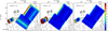 |
Fig. A.1 RMS noise for each of the 12CO J = 1− 0, 12CO J = 2− 1, and 13CO J = 1− 0 maps. All images are in the same colour scale, and the units in the colour bar are in Kelvin. Overlaid are the radio contours at 1420 MHz in units of brightness temperature at 4.8, 5.0, 5.5, and 6.0 K. The uneven rms values throughout our maps are due to us observing in many different weather and source elevation conditions. |
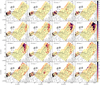 |
Fig. A.2 Tmb (K) for the 12CO J = 2− 1 line for the distant molecular cloud components, corresponding to velocities between − 27.5 and − 15.0 km s−1. Overlaid arethe radio contours at 1420 MHz in units of brightness temperature at 4.8, 5.0, 5.5, and 6.0 K. The velocities are indicated in the upper left corner of each panel. All figures in the same row share the same colour bar, plotted at the left end of each row. |
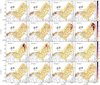 |
Fig. A.3 Tmb (K) for the 13CO J = 1− 0 line for the distant molecular cloud components, corresponding to velocities between − 27.5 and − 15.0 km s−1. Overlaid arethe radio contours at 1420 MHz in units of brightness temperature at 4.8, 5.0, 5.5, and 6.0 K. The velocities are indicated in the upper left corner of each panel. All figures in the same row share the same colour bar, plotted at the left end of each row. |
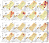 |
Fig. A.4 Tmb (K) for the 12CO J = 2− 1 (top), and 13CO J = 1− 0 (bottom) lines for the close molecular cloud components, corresponding to velocities between − 8.5 and − 1.0 km s−1. Overlaid are the radio contours at 1420 MHz in units of brightness temperature at 4.8, 5.0, 5.5, and 6.0 K. The velocities are indicated in the upper left corner of each panel. All figures in the same row share the same colour bar, plotted at the left end of each row. |
References
- Araya, M. 2013, MNRAS, 434, 2202 [NASA ADS] [CrossRef] [Google Scholar]
- Arias, M., Vink, J., Iacobelli, M., et al. 2019, A&A, 622, A6 [NASA ADS] [CrossRef] [EDP Sciences] [Google Scholar]
- Bobylev, V. V., & Bajkova, A. T. 2016, Astron. Lett., 42, 1 [NASA ADS] [CrossRef] [Google Scholar]
- Bocchino, F., Miceli, M., & Troja, E. 2009, A&A, 498, 139 [NASA ADS] [CrossRef] [EDP Sciences] [Google Scholar]
- Boumis, P., Akras, S., Leonidaki, I., et al. 2016, in Supernova Remnants: An Odyssey in Space after Stellar Death, 15 [Google Scholar]
- Burrows, D. N., & Guo, Z. 1994, ApJ, 421, L19 [NASA ADS] [CrossRef] [Google Scholar]
- Chen, Y., Seward, F. D., Sun, M., & Li, J.-T. 2008, ApJ, 676, 1040 [NASA ADS] [CrossRef] [Google Scholar]
- Chen, Y., Zhou, P., & Chu, Y.-H. 2013, ApJ, 769, L16 [NASA ADS] [CrossRef] [Google Scholar]
- Cox, D. P., Shelton, R. L., Maciejewski, W., et al. 1999, ApJ, 524, 179 [NASA ADS] [CrossRef] [Google Scholar]
- Dickman, R. L. 1978, ApJS, 37, 407 [NASA ADS] [CrossRef] [Google Scholar]
- Fesen, R. A., Blair, W. P., & Kirshner, R. P. 1985, ApJ, 292, 29 [NASA ADS] [CrossRef] [Google Scholar]
- Foster, T., & Brunt, C. M. 2015, AJ, 150, 147 [NASA ADS] [CrossRef] [Google Scholar]
- Guo, Z., & Burrows, D. N. 1997, ApJ, 480, L51 [NASA ADS] [CrossRef] [Google Scholar]
- Huang, Y.-L., & Thaddeus, P. 1986, ApJ, 309, 804 [NASA ADS] [CrossRef] [Google Scholar]
- Jiang, B., Chen, Y., Wang, J., et al. 2010, ApJ, 712, 1147 [NASA ADS] [CrossRef] [Google Scholar]
- Jurić, M., Ivezić, Ž., Brooks, A., et al. 2008, ApJ, 673, 864 [NASA ADS] [CrossRef] [MathSciNet] [Google Scholar]
- Kawamura, A., Onishi, T., Yonekura, Y., et al. 1998, ApJS, 117, 387 [NASA ADS] [CrossRef] [Google Scholar]
- Kawasaki, M., Ozaki, M., Nagase, F., Inoue, H., & Petre, R. 2005, ApJ, 631, 935 [NASA ADS] [CrossRef] [Google Scholar]
- Kothes, R., & Landecker, T. L. 2004, in The Magnetized Interstellar Medium, eds. B. Uyaniker, W. Reich, & R. Wielebinski (Katlenburg-Lindau: Copernicus GmbH), 33 [Google Scholar]
- Landecker, T. L., Pineault, S., Routledge, D., & Vaneldik, J. F. 1982, ApJ, 261, L41 [NASA ADS] [CrossRef] [Google Scholar]
- Landecker, T. L., Pineault, S., Routledge, D., & Vaneldik, J. F. 1989, MNRAS, 237, 277 [NASA ADS] [CrossRef] [Google Scholar]
- Lazendic, J. S., & Slane, P. O. 2006, ApJ, 647, 350 [NASA ADS] [CrossRef] [Google Scholar]
- Leahy, D., & Tian, W. 2005, A&A, 440, 929 [NASA ADS] [CrossRef] [EDP Sciences] [Google Scholar]
- Matsumura, H., Uchida, H., Tanaka, T., et al. 2017, PASJ, 69, 30 [NASA ADS] [CrossRef] [Google Scholar]
- Pineault, S., Pritchet, C. J., Landecker, T. L., Routledge, D., & Vaneldik, J. F. 1985, A&A, 151, 52 [NASA ADS] [Google Scholar]
- Pineault, S., Landecker, T. L., & Routledge, D. 1987, ApJ, 315, 580 [NASA ADS] [CrossRef] [Google Scholar]
- Reach, W. T., & Rho, J. 2000, ApJ, 544, 843 [NASA ADS] [CrossRef] [Google Scholar]
- Reach, W. T., Rho, J., Tappe, A., et al. 2006, AJ, 131, 1479 [NASA ADS] [CrossRef] [Google Scholar]
- Reid, M. J., Menten, K. M., Brunthaler, A., et al. 2014, ApJ, 783, 130 [Google Scholar]
- Rho, J., & Petre, R. 1998, ApJ, 503, L167 [NASA ADS] [CrossRef] [Google Scholar]
- Roberts, Jr. W. W. 1972, ApJ, 173, 259 [NASA ADS] [CrossRef] [Google Scholar]
- Seta, M., Hasegawa, T., Dame, T. M., et al. 1998, ApJ, 505, 286 [NASA ADS] [CrossRef] [Google Scholar]
- Taylor, A. R., Gibson, S. J., Peracaula, M., et al. 2003, AJ, 125, 3145 [NASA ADS] [CrossRef] [Google Scholar]
- van den Bergh, S., Marscher, A. P., & Terzian, Y. 1973, ApJS, 26, 19 [NASA ADS] [CrossRef] [Google Scholar]
- Vink, J. 2012, A&ARv, 20, 49 [Google Scholar]
- Weaver, R., McCray, R., Castor, J., Shapiro, P., & Moore, R. 1977, ApJ, 218, 377 [NASA ADS] [CrossRef] [Google Scholar]
- White, R. L., & Long, K. S. 1991, ApJ, 373, 543 [NASA ADS] [CrossRef] [Google Scholar]
- Wright, E. L., Eisenhardt, P. R. M., Mainzer, A. K., et al. 2010, AJ, 140, 1868 [NASA ADS] [CrossRef] [Google Scholar]
All Figures
|
Fig. 1 VRO 42.05.01 at 1420 MHz. This map taken from the CGPS. Labelled are the regions referred to throughout the text as “shell” (the small semicircle) and “wing” (the large triangle). We note that a sharp boundary separates the two regions. |
| In the text | |
|
Fig. 2 Tmb (K) for the 12CO J = 1− 0 transition for the distant molecular cloud components, corresponding to velocities between − 27.5 and − 15.0 km s−1. Overlaid arethe radio contours at 1420 MHz in units of brightness temperature at 4.8, 5.0, 5.5, and 6.0 K. The velocities are indicated in the upper left corner of each panel. All figures in the same row share the same colour bar, plotted at the left end of each row. |
| In the text | |
|
Fig. 3 Tmb (K) for the 12CO J = 1− 0 transition for the close molecular cloud components, corresponding to velocities between − 8.5 and − 1.0 km s−1. Overlaid arethe radio contours at 1420 MHz in units of brightness temperature at 4.8, 5.0, 5.5, and 6.0 K. The velocities are indicated in the upper left corner of each panel. All figures in the same row share the same colour bar, plotted at the left end of each row. |
| In the text | |
|
Fig. 4 Example of the fit that produces Fig. 5 for a single pixel. The data points from the cube are plotted in blue, the initial guess for the fit in dashed black, and the fit result is in red. The x-axis is in units of the cube velocity channels, where channel 200 corresponds to 0 km s−1, and channelsare 0.5 km s−1 apart. For this pixel the peaks are 0.785 K at − 21.6 km s−1 (channel 156.7), and at 0.508 K at − 4.2 km s−1 (channel 191.5). |
| In the text | |
|
Fig. 5 Results from fitting the distant (top) and close (bottom) components of the line profile to a Gaussian. For each of the two panels: height of the 12CO J = 1− 0 line in K (top, left), height of the 12CO J = 2− 1 line in K (top, middle), full-width at half maximum of the 12CO J = 1− 0 line in km s−1 (bottom, middle), full-width at half maximum of the 12CO J = 2− 1 line km s−1 (bottom, right), and best-fit central velocity in km s−1 (bottom, left). For regions with signal over 5σ, the ratio of 12CO J = 2− 1 to 12CO J = 1− 0 is plotted inthe top, right. Overlaid are the radio contours at 1420 MHz in units of brightness temperature at 4.8, 5.0, 5.5, and 6.0 K. Note the velocity gradient from the south to the north-west in the best-fit central velocity of the close component plot (lower left corner). The line used to make the position-velocity plot in Fig. 7 is indicated in this map in dark blue. |
| In the text | |
|
Fig. 6 From left to right, log of the optical depth of 13CO ( |
| In the text | |
|
Fig. 7 Position-velocity plot for a line that goes from RA = 5:25:50, Dec = +43:00:34 to RA = 5:25:09, Dec = +43:25:36 with a 72o inclination (see Fig. 5, lower-left corner) along the large velocity gradient seen at velocities of − 8 to − 2 km s−1. |
| In the text | |
|
Fig. 8 Averaged spectrum for the values in Fig. 5, blue plots, where the FWHM of the lines are greater than 3.5 km s−1. The fitting routine did not account for two clumps along the line-of-sight of a pixel for this range in velocities, and so tried to fit the two components as a single Gaussian with a broad FWHM (in green, corresponding to a FWHM of 4.4 km s−1). When we allowed for a second Gaussian term to be added to the model, the two clumps are fitted by Gaussians with narrow FWHM (1.62 km s−1). The data points from the cube are plotted in blue, the initial guess for the fit in dashed black, and the fit result is in red. The x-axis is in units of the cube velocity channels, where channel 200 corresponds to 0 km s−1, and channelsare 0.5 km s−1 apart. |
| In the text | |
|
Fig. 9 Best-fit central velocity for the close component (same as Fig. 5, lower left). Overlaid are the contours of VRO 42.05.01 in Hα at (5, 10, 20) × 10−17 ergs cm−2 s−1. It should be noted that the velocity gradient (which fades from yellow to green) appears to follow the semicircle (bright in Hα, and also in radio synchrotron) of the small shell of VRO 42.05.01. |
| In the text | |
|
Fig. 10 Distance from the Sun as a function of measured local standard of rest velocity as per Reid et al. (2014). The distant molecular component corresponds to distances between 2.25 and 8 kpc, and the close component corresponds to distances between 0.35 and 1.35 kpc. |
| In the text | |
|
Fig. 11 Velocity distribution of HI emission towards VRO 42.05.01 at the range of velocities that corresponds to the close molecular cloud. The data cube was taken from the CGPS. Overlaid are the radio contours at 1420 MHz in units of brightness temperature at 2.5, 3.7, 4.8, and 6 K. The wedges in the upper left corner of each plot correspond to the velocity of each slice. The brightness temperature TB colour scale is the same for all plots. |
| In the text | |
|
Fig. 12 3.4, 4.6, 12, and 22 μm (WISE, Wright et al. 2010), Hα and [S II] (Middlebury Emission-Line Atlas of Galactic SNRs, Winkler et al., in prep.) maps of VRO 42.05.01. Overlaid are the radio contours at 1420 MHz in units of brightness temperature at 4.8 and 6.0 K. |
| In the text | |
|
Fig. 13 12 μm WISE map with 1420 MHz radio contours in units of brightness temperature at 4.8 and 6.0 K. Labelled are the features we refer to in the body of the text. |
| In the text | |
|
Fig. A.1 RMS noise for each of the 12CO J = 1− 0, 12CO J = 2− 1, and 13CO J = 1− 0 maps. All images are in the same colour scale, and the units in the colour bar are in Kelvin. Overlaid are the radio contours at 1420 MHz in units of brightness temperature at 4.8, 5.0, 5.5, and 6.0 K. The uneven rms values throughout our maps are due to us observing in many different weather and source elevation conditions. |
| In the text | |
|
Fig. A.2 Tmb (K) for the 12CO J = 2− 1 line for the distant molecular cloud components, corresponding to velocities between − 27.5 and − 15.0 km s−1. Overlaid arethe radio contours at 1420 MHz in units of brightness temperature at 4.8, 5.0, 5.5, and 6.0 K. The velocities are indicated in the upper left corner of each panel. All figures in the same row share the same colour bar, plotted at the left end of each row. |
| In the text | |
|
Fig. A.3 Tmb (K) for the 13CO J = 1− 0 line for the distant molecular cloud components, corresponding to velocities between − 27.5 and − 15.0 km s−1. Overlaid arethe radio contours at 1420 MHz in units of brightness temperature at 4.8, 5.0, 5.5, and 6.0 K. The velocities are indicated in the upper left corner of each panel. All figures in the same row share the same colour bar, plotted at the left end of each row. |
| In the text | |
|
Fig. A.4 Tmb (K) for the 12CO J = 2− 1 (top), and 13CO J = 1− 0 (bottom) lines for the close molecular cloud components, corresponding to velocities between − 8.5 and − 1.0 km s−1. Overlaid are the radio contours at 1420 MHz in units of brightness temperature at 4.8, 5.0, 5.5, and 6.0 K. The velocities are indicated in the upper left corner of each panel. All figures in the same row share the same colour bar, plotted at the left end of each row. |
| In the text | |
Current usage metrics show cumulative count of Article Views (full-text article views including HTML views, PDF and ePub downloads, according to the available data) and Abstracts Views on Vision4Press platform.
Data correspond to usage on the plateform after 2015. The current usage metrics is available 48-96 hours after online publication and is updated daily on week days.
Initial download of the metrics may take a while.