| Issue |
A&A
Volume 627, July 2019
|
|
|---|---|---|
| Article Number | A90 | |
| Number of page(s) | 4 | |
| Section | The Sun | |
| DOI | https://doi.org/10.1051/0004-6361/201935216 | |
| Published online | 04 July 2019 | |
Interplanetary flux ropes of any twist distribution
1
Astronomical Institute of the Czech Academy of Sciences, Boční II 1401, 141 00 Praha 4, Czech Republic
e-mail: vandas@asu.cas.cz
2
Lamar University, Department of Physics, PO Box 10046, Beaumont, TX 77010, USA
e-mail: eromashets@lamar.edu
Received:
6
February
2019
Accepted:
27
May
2019
Context. Recent investigations indicate that the magnetic field configuration in interplanetary flux ropes is in contrast with the common magnetic field models that are used to fit them, namely constant-alpha force-free fields, whose twist increases without limits toward the flux-rope boundary. Therefore, magnetic field configurations with a constant twist are now being employed in fits.
Aims. Real flux ropes have varying twist. Therefore, analytical magnetic field configurations with prescribed twist distributions are searched for in cylindrical geometry.
Methods. Equations for the field solenoidality and for the force-free condition are solved for case when a twist profile is prescribed.
Results. A model of a force-free magnetic field configuration with an arbitrarily given twist distribution in a cylinder and its relative helicity per unit length are presented. It is applied to a core-envelope model recently suggested in studies of twist in magnetic clouds.
Key words: magnetic fields / Sun: coronal mass ejections (CMEs)
© ESO 2019
1. Introduction
Large interplanetary flux ropes were discovered in the 1970s and 1980s (Krimigis et al. 1976; Burlaga et al. 1981) and were named magnetic clouds (Klein & Burlaga 1982; Burlaga & Behannon 1982). For many years they were modeled by a constant-alpha force-free magnetic field in a cylinder (Burlaga 1988; Lepping et al. 1990, 2006, 2015; Farrugia et al. 1995; Marubashi & Lepping 2007), which had been found earlier by Lundquist (1950). In cylindrical coordinates (x = rcosφ, y = rsinφ, z = z) it reads

where B0 is the magnetic field magnitude at the axis (maximum) and J0 and J1 are the Bessel functions of the first kind, and zero and first orders, respectively. In recent years magnetic clouds started to be modeled by a uniform-twist force-free magnetic field in a cylinder (Wang et al. 2016, 2018), the so-called Gold-Hoyle tube (Gold & Hoyle 1960; Farrugia et al. 1999):

where B0 again is the magnetic field magnitude at the axis (maximum) and b is a constant.
These two field configurations represent to some extent two extremes for magnetic-field-line twists. Twist per unit length is defined as an angle that a field line makes around the magnetic axis within one unit length along it. Here both fields have Br zero, so each r = const. is a magnetic surface (i.e., these surfaces are concentric cylinders), and the magnetic field components depend on r alone, so the twist per unit length is given by
The twist for the Lundquist field increases without limit when r approaches the boundary of the flux rope, which is commonly defined as a place where Bz = 0; this immediately follows from Eq. (7). This fact and observations that interplanetary flux ropes have a rather flat twist distribution (Hu et al. 2015) lead to the modeling of magnetic clouds via the Gold-Hoyle tube, whose twist is exactly uniform, τ = b.
A uniform twist is an approximation because the twist will vary in real flux ropes (Hu et al. 2015; Wang et al. 2018; Yong et al. 2018; Zhao et al. 2018). We wondered if it is possible to construct a cylindrical flux rope with a given twist distribution. This task is solved in the next section.
2. Cylindrical flux rope with a prescribed twist
Similarly to the two field configurations mentioned, we assumed an axial symmetry, and

The component Bφ follows from Eq. (7)
where τ(r) is the prescribed profile of the twist. We note that the field is solenoidal for an arbitrary function Bz(r).
If field components are required to have a form similar to those of the Gold-Hoyle tube, then b is replaced by τ(r) in Eq. (6),
This field configuration is a Gold-Hoyle tube when τ = const., but it is a non-force-free field for other τ.
If we require the field to be force-free, then the force-free condition, rot B = α(r)B, yields for a general τ(r) an equation for Bz,
![$$ \begin{aligned} \tau (r) \left[r^2 \tau (r) B_z(r)\right]\prime + B_z\prime (r) = 0, \end{aligned} $$](/articles/aa/full_html/2019/07/aa35216-19/aa35216-19-eq11.gif)
where the prime is the derivative by r. The solution is
![$$ \begin{aligned} B_z&= B_0 \exp \left\{ -\int \limits _0^r \frac{\tau (\rho ) [\rho ^2 \tau (\rho )]\prime }{1+\rho ^2 \tau ^2(\rho )} \, \mathrm{d} \rho \right\} \nonumber \\&=\frac{B_0}{1+r^2\tau ^2(r)} \exp \left[\int \limits _0^r \frac{\rho ^2 \tau (\rho ) \tau \prime (\rho )}{1+\rho ^2 \tau ^2(\rho )} \, \mathrm{d} \rho \right] ,\end{aligned} $$](/articles/aa/full_html/2019/07/aa35216-19/aa35216-19-eq12.gif)
where the prime is the derivative by ρ. We get for α
where the prime is the derivative by r. When τ(r) = b, Eq. (12) immediately yields Eq. (6). And for τ(r) = J1(αr)/[rJ0(αr)], which is the twist per unit length for the Lundquist field (cf. Dasso et al. 2003, Eq. (4)) the integral in Eq. (12) can also be analytically evaluated, and we get Eq. (3).
We note that the solution for a cylindrical flux rope, given by Eqs. (8), (9), and (12), can be generalized for a toroidal flux rope. Using the same approach as by Vandas & Romashets (2017), we obtain in toroidally curved cylindrical coordinates [x = (R0 + rcosθ) cosφ, y = (R0 + rcosθ) sinφ, z = rsinθ]


Here R0 is the toroid’s major radius, and the function G(r) is Bz/B0 from Eq. (12), where r is now interpreted as a coordinate of toroidally curved cylindrical system. The field is exactly solenoidal and approximately force-free (for large R0).
The helicity of this toroidal flux rope is
where r0 is the toroid’s minor radius. Helicity per unit length is
To obtain relative helicity per unit length for our cylindrical flux rope, we make a limit R0 → ∞. Because Hl from Eq. (18) does not depend on R0, the relative helicity is just this value of Hl. It is essentially a triple integral. For τ(r) = b we have G(r) = (1 + b2r2)−1, Eq. (18) can be analytically evaluated, and we obtain the formula for the relative helicity per unit length of the Gold-Hoyle tube, presented by Dasso et al. (2003, Eq. (9)).
3. Core-envelope model of a cylindrical flux rope
Hu et al. (2015) presented profiles of twist in magnetic clouds. There is a small core with a relatively high twist and an envelope with a fairly flat twist profile, slightly increasing towards the boundary (e.g., Hu et al. 2015, Fig. 8). We modeled this profile with a function
It has a Gaussian core with the twist a at the axis, b is a level of twist in the envelope, δ defines its slight increase towards the boundary. The parameter γ determines a compactness of the core. Figure 1 shows plots of this function for two sets of parameters, the first with γ = 10 (in red) and the second with γ = 20 (in blue). The second case is supplemented by a dependence on the magnetic surfaces A (dashed line) in order to have a direct comparison with Fig. 8 in Hu et al. (2015). The magnetic surfaces A are given in our case by the formula  .
.
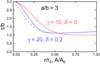 |
Fig. 1. Profiles of the twist given by Eq. (19) for two sets of parameters: a/b = 3, δ = 0.2, and γ = 20 (in blue), and a/b = 3, δ = 0, and γ = 10 (in red). Solid lines indicate the profiles as a function of r, the dashed line as a function of magnetic surfaces A. |
Figure 2a shows profiles of the magnetic field components and field magnitude for the treated model (in blue), which we call the core-envelope model. The field components were calculated from Eqs. (8), (9), and (12). Integration with τ from Eq. (19) was done numerically. With current computers it is a fast task. The profiles are supplemented for comparison by that of the uniform-twist model (Gold-Hoyle tube, in red), whose twist is characteristic of the envelope (i.e., equal to b). We see that the profiles are quite different.
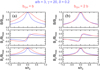 |
Fig. 2. Magnetic field profiles along the x-axis for the core-envelope model (blue lines). They are supplemented (panel a) by the profiles of the Gold-Hoyle tube with the twist bGH = b, which is characteristic of the envelope, or (panel b) by the profiles of the Gold-Hoyle tube with the twist doubled, bGH = 2b. Bx = 0 for all cases, so it is not shown. The magnetic values are scaled by Bmax, which is the maximum field magnitude (the value at the flux-rope axis). |
We note that we adopted the terms core and envelope used by Hu et al. (2015). There is also another core-envelope model of magnetic clouds that is not related to the present one. It was introduced by R. P. Lepping (Lepping et al. 2006); it concerns the Lundquist flux rope, where the core is the central part with one Bz polarity and the envelope has the opposite polarity. The twist is infinite on the core-envelope boundary in this model.
Wang et al. (2016) made fits of many magnetic clouds by the Gold-Hoyle tube and determined their twists bGH. They compared them with twists following from other methods (like the Grad-Shafranov reconstruction or the analysis of energetic electron motions). They concluded that the twists bGH are 1.5–2.5× larger than follow from other methods. We examined this problem in frame of the core-envelope model. Magnetic field profiles of this model in Fig. 2a are overlayed by profiles of the Gold-Hoyle tube with the same level of twist as it is in the envelope. Considering the red profiles as a fit to the blue profiles, that is, a fit of the core-envelope field by the uniform-twist field, we conclude that it is a very bad fit. Interestingly, when we increase the uniform twist twice, i.e., bGH = 2b, we get a fairly good fit, as is shown in Fig. 2b.
We use this value of bGH as an example; it is possible to do it more rigorously and search for a minimum of the expression
![$$ \begin{aligned} \Delta B = \sqrt{\frac{1}{N} \sum \limits _{i=1}^N [\boldsymbol{B}_{\mathrm{GH} ,i}-\boldsymbol{B}_i]^2} , \end{aligned} $$](/articles/aa/full_html/2019/07/aa35216-19/aa35216-19-eq21.gif)
that is similar to the case when observations are fit. Here N is the number of points at the x-axis for comparison. The minimum exists and is well expressed, as can be seen in Fig. 3a. For reasonable parameters the minima for bGH/b are around 2–3.
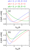 |
Fig. 3. Value of Δ as a function of bGH of the Gold-Hoyle tube which fits a core-envelope flux rope, the parameters of which are kept constant. Δ characterizes deviations of the two field profiles scaled by their field-magnitude maxima, and it corresponds to the quantity χ used when real observations of magnetic clouds are compared to models (e.g., Lepping et al. 2006). Results for three sets of parameters of the core-envelope model, shown at the top, are plotted and indicated by color. Panel a is for a central crossing, while panel b is for a crossing in a distance of 0.2 r0 from the magnetic axis. |
The presented comparison is made for a central crossing where this effect is the most pronounced. Here a spacecraft scans a higher-twist core in the whole. For non-central crossings this effect is weakened depending on how far from the magnetic axis a spacecraft passes. Figure 3b is for a passage 0.2 r0 from the axis. The cases are the same as for the central crossing shown in the panel a. We see that the minima are again well expressed, but the twist ratios are shifted toward lower values. Supposing that a majority of magnetic cloud events are passages not far from the magnetic axis (in which case magnetic clouds are well identified), the discussed effect can contribute to the disagreement found by Wang et al. (2016).
4. Conclusions
A model of a force-free field with varying prescribed twist in a cylinder was derived. Based on an observationally determined twist distribution, a core-envelope force-free model of a cylindrical flux rope was presented. This model may contribute to an explanation of why a fit with a constant twist yields a twist that is about two times higher than it actually is (as reported by Wang et al. 2016). The presented model is not limited to core-envelope twist distributions, but may describe other twist distributions revealed by recent studies (Wang et al. 2018; Zhao et al. 2018) or forthcoming studies.
Acknowledgments
M.V. acknowledges support from Grant 17-06065S by the Grant Agency of the Czech Republic and from the AV ČR Grant RVO:67985815.
References
- Burlaga, L. F. 1988, J. Geophys. Res., 93, 7217 [NASA ADS] [CrossRef] [Google Scholar]
- Burlaga, L. F., & Behannon, K. W. 1982, Sol. Phys., 81, 181 [NASA ADS] [CrossRef] [Google Scholar]
- Burlaga, L., Sittler, E., Mariani, F., & Schwenn, R. 1981, J. Geophys. Res., 86, 6673 [Google Scholar]
- Dasso, S., Mandrini, C. H., Démoulin, P., & Farrugia, C. J. 2003, J. Geophys. Res., 108 [Google Scholar]
- Farrugia, C. J., Osherovich, V. A., & Burlaga, L. F. 1995, J. Geophys. Res., 100, 12293 [NASA ADS] [CrossRef] [Google Scholar]
- Farrugia, C. J., Janoo, L. A., Tobert, R. B., et al. 1999, in Solar Wind Nine, eds. S. R. Habbal, R. Esser, J. V. Hollweg, & P. A. Isenberg (Woodbury, New York: AIP), AIP Conf. Proc., 471, 745 [NASA ADS] [CrossRef] [Google Scholar]
- Gold, T., & Hoyle, F. 1960, MNRAS, 120, 89 [NASA ADS] [Google Scholar]
- Hu, Q., Qiu, J., & Krucker, S. 2015, J. Geophys. Res., 120, 5266 [Google Scholar]
- Klein, L. W., & Burlaga, L. F. 1982, J. Geophys. Res., 87, 613 [Google Scholar]
- Krimigis, S., Sarris, E., & Armstrong, T. 1976, Trans. AGU, 57, 304 [Google Scholar]
- Lepping, R. P., Jones, J. A., & Burlaga, L. F. 1990, J. Geophys. Res., 95, 11957 [NASA ADS] [CrossRef] [Google Scholar]
- Lepping, R. P., Berdichevsky, D. B., Wu, C.-C., et al. 2006, Ann. Geophys., 24, 215 [NASA ADS] [CrossRef] [Google Scholar]
- Lepping, R. P., Wu, C.-C., & Berdichevsky, D. B. 2015, Sol. Phys., 290, 553 [NASA ADS] [CrossRef] [Google Scholar]
- Lundquist, S. 1950, Ark. Fys., 2, 361 [Google Scholar]
- Marubashi, K., & Lepping, R. P. 2007, Ann. Geophys., 25, 2453 [NASA ADS] [CrossRef] [Google Scholar]
- Vandas, M., & Romashets, E. 2017, A&A, 608, A118 [NASA ADS] [CrossRef] [EDP Sciences] [Google Scholar]
- Wang, Y., Zhuang, B., Hu, Q., et al. 2016, J. Geophys. Res., 121, 9316 [CrossRef] [Google Scholar]
- Wang, Y., Shen, C., Liu, R., et al. 2018, J. Geophys. Res., 123, 3238 [Google Scholar]
- Yong, J. H., Liu, C.-M., Peng, J., et al. 2018, J. Geophys. Res., 123, 7167 [Google Scholar]
- Zhao, A., Wang, Y., Feng, H., et al. 2018, ApJ, 869, L13 [NASA ADS] [CrossRef] [Google Scholar]
All Figures
|
Fig. 1. Profiles of the twist given by Eq. (19) for two sets of parameters: a/b = 3, δ = 0.2, and γ = 20 (in blue), and a/b = 3, δ = 0, and γ = 10 (in red). Solid lines indicate the profiles as a function of r, the dashed line as a function of magnetic surfaces A. |
| In the text | |
|
Fig. 2. Magnetic field profiles along the x-axis for the core-envelope model (blue lines). They are supplemented (panel a) by the profiles of the Gold-Hoyle tube with the twist bGH = b, which is characteristic of the envelope, or (panel b) by the profiles of the Gold-Hoyle tube with the twist doubled, bGH = 2b. Bx = 0 for all cases, so it is not shown. The magnetic values are scaled by Bmax, which is the maximum field magnitude (the value at the flux-rope axis). |
| In the text | |
|
Fig. 3. Value of Δ as a function of bGH of the Gold-Hoyle tube which fits a core-envelope flux rope, the parameters of which are kept constant. Δ characterizes deviations of the two field profiles scaled by their field-magnitude maxima, and it corresponds to the quantity χ used when real observations of magnetic clouds are compared to models (e.g., Lepping et al. 2006). Results for three sets of parameters of the core-envelope model, shown at the top, are plotted and indicated by color. Panel a is for a central crossing, while panel b is for a crossing in a distance of 0.2 r0 from the magnetic axis. |
| In the text | |
Current usage metrics show cumulative count of Article Views (full-text article views including HTML views, PDF and ePub downloads, according to the available data) and Abstracts Views on Vision4Press platform.
Data correspond to usage on the plateform after 2015. The current usage metrics is available 48-96 hours after online publication and is updated daily on week days.
Initial download of the metrics may take a while.