| Issue |
A&A
Volume 627, July 2019
|
|
|---|---|---|
| Article Number | A18 | |
| Number of page(s) | 11 | |
| Section | The Sun | |
| DOI | https://doi.org/10.1051/0004-6361/201935048 | |
| Published online | 25 June 2019 | |
Effect of the non-uniform solar chromospheric Lyα radiation on determining the coronal H I outflow velocity
1
INAF–Catania Astrophysical Observatory, Via Santa Sofia 78, 95123 Catania, Italy
e-mail: sergio.dolei@inaf.it
2
INAF–Turin Astrophysical Observatory, Via Osservatorio 20, 10025 Pino Torinese (TO), Italy
3
INAF–Capodimonte Astronomical Observatory, Salita Moiariello 16, 80131 Napoli, Italy
4
CNR–Institute of Photonics and Nanotechnologies, Via Trasea 7, 35131 Padova, Italy
5
INAF–Arcetri Astrophysical Observatory, Largo Enrico Fermi 5, 50125 Firenze, Italy
6
University of Padova–Dept. of Physics and Astronomy, Via Marzolo 8, 35131 Padova, Italy
7
University of Florence–Dept. of Physics and Astronomy, Largo Enrico Fermi 2, 50125 Firenze, Italy
Received:
11
January
2019
Accepted:
22
May
2019
We derived maps of the solar wind outflow velocity of coronal neutral hydrogen atoms at solar minimum in the altitude range 1.5–4.0 R⊙. We applied the Doppler dimming technique to coronagraphic observations in the UV H I Lyα line at 121.6 nm. The technique exploits the intensity reduction in the coronal line with increasing velocities of the outflowing plasma to determine the solar wind velocity by iterative modelling. The Lyα line intensity is sensitive to the wind outflow velocity and also depends on the physical properties of coronal particles and underlying chromospheric emission. Measurements of irradiance by the chromospheric Lyα radiation in the corona are required for a rigorous application of the Doppler dimming technique, but they are not provided by past and current instrumentations. A correlation function between the H I 121.6 nm and He II 30.4 nm line intensities was used to construct Carrington rotation maps of the non-uniform solar chromospheric Lyα radiation and thus to compute the Lyα line irradiance throughout the outer corona. Approximations concerning the temperature of the scattering H I atoms and exciting solar disc radiation were also adopted to significantly reduce the computational time and obtain a faster procedure for a quick-look data analysis of future coronagraphic observations. The effect of the chromospheric Lyα brightness distribution on the resulting H I outflow velocities was quantified. In particular, we found that the usual uniform-disc approximation systematically leads to an overestimated velocity in the polar and mid-latitude coronal regions up to a maximum of about 50−60 km s−1 closer to the Sun. This difference decreases at higher altitudes, where an increasingly larger chromospheric portion, including both brighter and darker disc features, contributes to illuminate the solar corona, and the non-uniform radiation condition progressively approaches the uniform-disc approximation.
Key words: Sun: corona / solar wind / Sun: UV radiation
© ESO 2019
1. Introduction
Over many decades, the main target of theoretical and observational solar wind studies has been comprehending the basic physical processes that give rise to the formation and expansion of the solar wind. Many topics still need a general clarification, such as the identification of the outer coronal region where the larger acceleration of particles occurs. For this purpose, it is important to keep in mind the close correlation between solar wind dynamics and the physical mechanisms that are responsible for coronal heating. Therefore, addressing the problem of the solar wind acceleration requires determining the wind outflow velocities in a range of heliocentric distances between 1 and 10 R⊙, as well as reliable measurements of kinetic temperatures for different species, depending on both their thermal and non-thermal motions.
One of the methods for determining the solar wind velocity is based on the so-called Doppler dimming technique (Beckers & Chipman 1974; Hyder & Lytes 1970; Noci et al. 1987; Withbroe et al. 1982), which is applied to ultraviolet (UV) spectrometric observations. This technique takes into account the progressive reduction of the resonantly scattered component of the coronal UV H I Lyα line with increasing outflow velocities. The Lyα line intensity is sensitive to the velocity of the outflowing plasma from about 50 to 400 km s−1 (see e.g. Dolei et al. 2018). The dimming effect is negligible for velocities lower than 50 km s−1, whereas the resonantly scattered component of the Lyα line is completely dimmed for velocities higher than 400 km s−1 (see e.g. Withbroe et al. 1982). It is worth noting that these values are the typical velocities for neutral hydrogen atoms in the outer corona (Dolei et al. 2015, 2018; Spadaro et al. 2007; Susino et al. 2008), confirming that the Doppler dimming technique is a suitable method for investigating the solar wind that flows out through these coronal regions.
The outer solar corona has been extensively investigated by space- and ground-based observations that were performed by many different instruments, mostly in the past 20 years with the UltraViolet Coronagraph Spectrometer (UVCS; Kohl et al. 1995) on board the SOlar and Heliospheric Observatory (SOHO; Domingo et al. 1995). This instrument performed UV spectrometric observations of the H I Lyα line (121.6 nm) and O VI resonance doublet (103.2 and 103.7 nm) over a time interval that is longer than a whole solar activity cycle (1996–2012). It provided measurements of line intensities and kinetic temperatures for the atomic species at different altitudes and latitudes (Cranmer et al. 1999; Kohl et al. 1997; Noci et al. 1997a,b), thus giving a unique contribution to the scientific questions of solar wind acceleration and coronal heating (see e.g. Antonucci et al. 2012; Kohl et al. 2006, for a review of these results). The future missions to the Sun, and in general, the study of the solar corona, will benefit from the heritage of knowledge that was significantly enriched by the results of this spectrocoronagraphic investigation.
Very recently, Dolei et al. (2018) used UVCS/SOHO observations to obtain daily maps of the H I outflow velocity over a complete solar rotation in June 1997 by means of the Doppler dimming technique. They derived the intensity of the resonantly scattered H I Lyα line, starting from some considerations about the physical and geometrical properties that characterise the chromospheric and coronal environments. The same dataset was analysed by Bemporad (2017) to infer dynamical information on the solar wind acceleration processes. Both authors assumed total intensity and a shape of the profile of the exciting solar disc Lyα radiation as seen by the scattering atoms along the line of sight. In particular, the chromospheric intensity was assumed to be uniform over the entire disc. However, observations performed by SWAN/SOHO (Bertaux et al. 1995) provide evidence of non-uniform illumination of the corona and heliosphere by the Lyα disc (Bertaux et al. 2000). Auchère (2005) quantified the ratio at different altitudes in polar coronal holes between the intensity of the resonantly scattered Lyα line computed at solar minimum in the cases of uniform and non-uniform disc, assuming a standard outflow velocity radial profile taken from the literature. He found that the uniform-disc approximation systematically leads to an overestimated coronal Lyα intensity by a factor of 15% on average, depending on the distribution of the brighter (e.g. active regions) and darker (e.g. coronal holes) disc features.
Measurements of total solar irradiance in the Lyα line are very important because this is the strongest line in the extreme UV (EUV) solar spectrum and because it is primarily responsible for the formation of the Earth’s ionosphere. In the past and at present, the Lyα irradiance has been monitored by many instruments, such as XPS/SORCE (Woods et al. 2005), SOLSTICE/UARS (Rottman & Woods 1994), and most recently, LYRA/PROBA2 (Dominique et al. 2013), which perform an integration of the Lyα intensity over the entire solar disc. However, the application of the Doppler dimming technique requires knowing the inhomogeneities in the Lyα intensity distribution on the Sun’s chromosphere as seen by the coronal H I atoms. In the future, the chromospheric Lyα distribution will be measured by the EUI instrument (Rochus et al., in prep.) for the Solar Orbiter mission (Müller et al. 2013, and in prep.), but the observations will be acquired in a limited field of view (about 0.3 R⊙ at the closest approach of the spacecraft), which is insufficient to provide global maps of the Lyα intensity on the Sun.
In this scenario, the objective of the present work is to evaluate the effect of chromospheric radiation inhomogeneities on the determination of the solar wind outflow velocity. It is an extension of the work of Dolei et al. (2018), which was aimed at deriving velocity maps of the H I atoms at solar minimum by applying the Doppler dimming technique in the uniform-disc approximation. Here we adopt an improved version of their procedure, including measurements of the local Lyα intensity variation on the solar disc obtained by chromospheric observations. In addition, we provide detailed functional forms that can suitably be used for the synthesis of the coronal resonantly scattered Lyα line intensity on the basis of the specific physical properties of the solar chromosphere and corona (see Appendix A). Our results may provide useful support to the investigations that will be performed with future coronagraphic instruments and contribute to solve the problem of solar wind acceleration.
2. Doppler dimming effect on the resonantly scattered Lyα line radiation in the solar corona
2.1. Doppler dimming technique
The emission of the UV H I Lyα line in the solar corona is produced by collisional and radiative mechanisms, the first of which generally accounts only for a negligible fraction of the total radiation (Gabriel 1971; Raymond et al. 1997). Only in the case of coronal mass ejections (CMEs) can the contribution of the collisional component become significant (see e.g. Susino et al. 2018). The functional form of the radiative component of the Lyα line intensity that results from the resonant scattering of chromospheric radiation by neutral hydrogen atoms can be deduced for instance by following the approach of Withbroe et al. (1982) and Noci et al. (1987). If at a coronal point P, H I atoms with a certain radial outflow velocity υ absorb chromospheric Lyα photons that come from a direction n′ and then emit them towards an observer in a direction n, the intensity (or radiance, in units of erg cm−2 s−1 sr−1) measured along the line of sight is given by
where h is the Planck constant, B12 is the Einstein coefficient for the absorption related to the spectral transition with central wavelength λ0 = 121.6 nm, ne is the coronal electron density, Ri is the neutral hydrogen ionisation fraction (depending on the coronal electron temperature Te), x is the spatial coordinate along the line of sight, Ω is the solid angle under which point P subtends the solar disc, 𝒥(λ′,n′) is the specific intensity of the chromospheric Lyα radiation at wavelength λ′ that depends on the incoming direction n′, and Φ is the Lyα absorption profile of the coronal scattering H I atoms. The shape of Φ is mainly determined by the kinetic temperature of the H I atoms (THI), resulting from their thermal and non-thermal motions. The probability that the chromospheric radiation is absorbed by the coronal atoms depends on the Doppler shift λ = λ0(1 + υ ⋅ n′/c) that is caused by the velocity υ, where c is the speed of light. When the corona is in a static condition, the exciting chromospheric radiation profile and the coronal absorption profile are centred at the same wavelength (λ′=λ = λ0), which means that they produce the maximum intensity of the resonantly scattered Lyα line. Instead, when the corona expands with a certain outflow velocity, the incident radiation profile appears to be Doppler shifted in the rest frame of the scattering atoms, and a lower rate of resonant scattering processes occurs. The Lyα line intensity progressively decreases with increasing outflow velocities and appears to be almost completely dimmed at about 400 km s−1, which thus is an upper limit for the velocity that can be measured for H I atoms (see e.g. Dolei et al. 2018; Withbroe et al. 1982).
The intensity of the resonantly scattered Lyα line can be synthesised using the Eq. (1) after the physical quantities are suitably assumed or independently determined. From comparing it with the Lyα intensity measured by UV observations, which is sensitive to the plasma velocity, the outflow velocity can be derived by iterative modelling. The synthetic intensity can be obtained by tuning the velocity value until the observations are reproduced. In so doing, the best match between synthetic and observed Lyα line intensity will provide an estimate of the solar wind H I outflow velocity.
2.2. Deriving physical parameters
The computation of the coronal Lyα line intensity requires knowing the physical quantities involved in the Lyα resonant scattering process, which are denoted in the above equations by the parameters ne, Ri = Ri(Te), Φ = Φ(THI), and 𝒥(λ′,n′). Except for the chromospheric Lyα radiation, which is obtained by a more elaborated data analysis and is discussed in a dedicated paragraph of the next section, the assumptions and procedures we employed in the definition of these quantities are described below.
2.2.1. Coronal electron density
The coronal electron density ne was derived by means of the Van De Hulst inversion technique (Van De Hulst 1950) applied to full-corona images in polarised visible light (VL). The technique allows obtaining electron density radial profiles at all latitudes that better reproduce the VL polarised brightness (pB), which is produced by Thomson scattering of the solar disc Lyα radiation by coronal electrons (see Hayes et al. 2001; Dolei et al. 2018 for a more detailed description of this method).
2.2.2. Coronal electron temperature
The ratio Ri between neutral and ionised hydrogen atoms is a function of the coronal electron temperature Te, which is responsible for the population of the ions. The dependence of Ri on Te is stronger at lower altitudes, where the ionisation equilibrium is reached. As first pointed out by Withbroe et al. (1982), the collisional ionisation time for neutral hydrogen is longer than the coronal expansion time above 8 R⊙ in the equatorial streamers and above 3 R⊙ in the polar coronal holes, and Ri becomes almost constant with altitude. In this work the radial variation of the electron temperature in the outer coronal region was obtained by an average between the Te radial profiles provided at solar minimum by Gibson et al. (1999) for an equatorial streamer and by Vasquez et al. (2003) for polar regions (see Dolei et al. 2018 for more details).
2.2.3. Neutral hydrogen kinetic temperature
The Lyα line absorption profile Φ of the coronal neutral hydrogen atoms is determined by various contributions: thermal and non-thermal plasma motions, and natural line broadening. The latter contribution is negligible in the line core and at the low plasma densities characterising the solar wind. Measurements of the coronal Lyα line widths, corrected for instrumental effects and possible contamination by interplanetary Lyα emission (negligible below 4–5 R⊙, see e.g. Spadaro et al. 2017), provide information on the neutral hydrogen velocity distribution, which is a function of the kinetic temperature. The H I temperature distribution in the outer corona is anisotropic, especially in coronal holes, as found by many different authors on the basis of the UVCS data analysis (see Kohl et al. 2006 and references therein). Nevertheless, Dolei et al. (2016, 2018) recently found that the neutral hydrogen outflow velocities weakly depend on the H I temperature, and in particular on the assumed degree of anisotropy, because the velocity differences are about 10% at most. Therefore, we assumed that the H I temperature is isotropic, and its radial and latitudinal distribution are given by the map shown in Fig. 1. This map was obtained with the procedure that was first proposed by Dolei et al. (2018), who took a large collection of UVCS Lyα observations over different time windows at solar minimum into account. Cylindrical symmetry was assumed for the solar corona in order to remove possible bias on the resulting outflow velocities that is caused by certain temperature distributions that derive from the analysis of the considered UVCS dataset. More specifically, we calculated weighted averages of the temperature values that were obtained at the same altitude and latitude (both positive and negative) by interpolating and extrapolating the UVCS data, as described in detail in Dolei et al. (2016, 2018). The adopted weight is given by the difference between each temperature value and the mean temperature over the map. We replaced the initial temperature values with the resulting averages, and finally applied a radial fit to the average data using the functional form given by Vasquez et al. (2003) that is reported in Eq. (1) of Dolei et al. (2016). It is worth remarking that the reconstructed H I temperature map was obtained from numerous observations at solar minimum and is not aimed to reproduce a real coronal configuration. The map also presents some darker areas in the mid-latitude regions, resulting from the extrapolation procedure carried out up to altitudes where observational data are missing. On the other hand, this map is helpful for our purposes and gives an idea of the temperature distribution in the outer corona. The H I temperature map covers all latitudes in the range of heliocentric distances between 1.5 and 4.0 R⊙. This range is mainly constrained by the altitudes that were investigated by the original UVCS observations and corresponds to the portion of the outer corona in which the outflow velocities are derived in the present work.
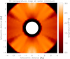 |
Fig. 1. Reconstructed H I temperature map at solar minimum. |
3. Observations and data analysis
Two-dimensional (hereafter 2D) maps of the solar wind H I outflow velocity were obtained in the outer corona. We here use part of the dataset that was investigated by Bemporad (2017) and Dolei et al. (2018). These authors constructed continuous coronagraphic UV and VL images, applied the Doppler dimming technique, and derived 2D velocity maps over a complete solar rotation in June 1997 by assuming the uniform-disc approximation. In contrast, we here obtained the intensity and distribution of the solar disc Lyα radiation from chromospheric observations. The solar disc data provide measurements of the local intensity variation and allow us to evaluate the effect of the non-uniform chromospheric radiation on the derived outflow velocities.
3.1. Coronagraphic UV and VL images
Full-corona 2D images were obtained from UV and VL data acquired on 1997 June 7, 14, 18, and 21, that is, during the minimum phase between solar cycles 22 and 23. In particular, we reconstructed resonantly scattered Lyα line intensity images using UVCS/SOHO synoptic spectrometric observations, and VL polarised brightness images by combining observations acquired by the Large Angle and Spectrometric COronagraph (LASCO; Brueckner et al. 1995) on board SOHO, and the Mark-III K-Coronameter (Mk3; Fisher et al. 1981) that is installed at the Mauna Loa Solar Observatory (MLSO). Continuous coverage in the altitude range 1.5–4.0 R⊙ was achieved by interpolation and extrapolation of the original data, as explained in detail by Bemporad (2017) and Dolei et al. (2018).
3.2. Chromospheric Lyα Carrington maps
We derived the 2D outflow velocity maps by computing the resonantly scattered H I Lyα line intensity throughout the solar corona. This in turn requires determining the co-temporal distribution of the exciting Lyα radiation on the Sun. Acquisition of coronal and chromospheric data very close in time is fundamental in the study of solar wind dynamics. The variations in total Lyα radiation of the solar disc over the solar activity cycle are significant (see Lemaire et al. 2015, for cyclic variations in the time interval 1996–2009) and thus potentially affect the determination of the wind velocities. One possibility is to use Carrington maps of chromospheric emission that corresponds to Carrington rotations that include the time interval that is covered by the selected days in June 1997. A Carrington map is generally built by taking intensity profiles along the central meridian of full-disc images over 27 consecutive days and placing them next to each other after correcting for the cosine distortion with heliographic latitude. The Carrington map is not a rigorous representation of the daily solar surface and neglects the temporal evolution of solar features and transient events, such as flares and CMEs. However, it provides a suitable distribution map of the chromospheric Lyα line radiation over the entire solar disc. Unfortunately, there is at present a lack of systematic full-disc Lyα observations that prevents us from constructing Carrington maps. Nevertheless, Auchère (2005) established a correlation function between the total intensities of the H I line at 121.6 nm and He II line at 30.4 nm on the solar disc. This relationship can be used to convert He II images into H I Lyα images. In following this approach, we exploited Carrington rotation maps 1923 and 1924 that were constructed by Benevolenskaya et al. (2001) using the solar disc observations in the He II 30.4 nm narrow-bandpass filter acquired with the Extreme-ultraviolet Imaging Telescope (EIT; Delaboudinière et al. 1995) on board SOHO from 1997 May 22 to July 15. The EIT provided full-disc images in four narrow passbands (about 1.5 nm wide) of the EUV spectrum centred at 17.1, 19.5, 28.4, and 30.4 nm (He II spectral line emission), with a spatial resolution of about 5″. In general, Benevolenskaya et al. (2001) obtained calibrated Carrington maps in the He II line intensity with a spatial resolution of 1°, in longitude from 0° to 360° and latitude from −83° to +83°. We extended the latitude range down to −90° and up to +90° by replacing the missing data with the mean values computed over any longitude between −83° and −80°, and between +80° and +83°, respectively. Conversion from instrumental into physical units was performed after correcting for the contamination by other line emission in the EIT 30.4 nm bandpass filter (Cook et al. 1999; Dere et al. 2000). Figure 2 shows the composite image of Carrington rotation maps 1923 and 1924 in the He II 30.4 nm line. This image was converted into the analogous image in the H I Lyα line using the correlation function given by Auchère (2005),
![$$ \begin{aligned} \mathcal{J} _{121.6}=436\,[1-0.955\exp (-0.0203\,\mathcal{J} _{30.4})], \end{aligned} $$](/articles/aa/full_html/2019/07/aa35048-19/aa35048-19-eq2.gif)
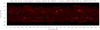 |
Fig. 2. Carrington rotation maps 1923 and 1924 in the He II 30.4 nm line. The intensity range extends from 2.3 to 335.6 W m−2 sr−1. |
where the intensities 𝒥 are in units of W m−2 sr−1. From the composite image in Lyα line intensity (see Fig. 3), we extracted individual Carrington maps centred at the location of the central meridian in a given date from 1997 May 22 to July 15, in order to reduce the time gap between the original observations and the selected date down to 13–14 days. Figure 4 specifically shows the four Carrington maps for the investigated days in June 1997.
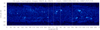 |
Fig. 3. Carrington rotation maps 1923 and 1924 in the H I Lyα line. The intensity range extends from 38.8 to 435.5 W m−2 sr−1. The vertical dashed white lines mark the location of the central meridian on 1997 June 7, 14, 18, and 21 from right to left, respectively. |
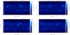 |
Fig. 4. H I Lyα Carrington maps centred at the location of the central meridian on 1997 June 7, 14, 18, and 21, respectively. Coronal plasma outflowing on the POS is mainly illuminated by the solar disc regions around −90° longitude (east limb) and +90° longitude (west limb). |
It is important to take into account that the conversion from He II 30.4 nm images into H I 121.6 nm images is only based on the correlation between the total full-disc intensity at the two wavelengths. The spectral emission of individual features on the solar surface (sunspots, spicules, flares, etc.) is not considered. As a consequence, the global morphology of the Sun could appear different in the two lines. Systematic investigations of solar disc features at 17.1 nm and 121.6 nm have revealed similar morphologies at these wavelengths, which suggests a physical link between their coronal and chromospheric emissions (Vourlidas et al. 2001). To exclude a different behaviour between the He II 30.4 nm and H I 121.6 nm line emissions, we can restrict our investigation to the morphology of the chromosphere over a single day. In particular, we benefit from the full-disc Lyα image reported in Fig. 3 of Akinari (2008). This was reconstructed from the UVCS disc measurements on the 1997 October 8 and can be used for a comparison with the analogous image derived from the EIT 30.4 nm observations. The EIT data were calibrated by means of the EIT_PREP.pro routine of the standard SolarSoftware package in Interactive Data Language (IDL) environment. Figure 5 shows the chromospheric H I Lyα image obtained from the He II 30.4 nm image after conversion into physical units and application of the correlation function in Eq. (2). Despite the different spatial resolution of the UVCS data (14″ and 24″ along and across the UVCS slit, respectively), this image and that of Akinari (2008) show very similar morphologies and intensity scales (in a range from 4 × 10¹⁴ to 1.5 × 10¹⁶ photons cm−2 s−1 sr−1), in particular for the quiet Sun and active regions. This evidence supports the use of the correlation function between the total full-disc intensities of the two UV spectral lines in order to study the effect of the local Lyα intensity variation. On the other hand, the contrast in the polar coronal holes appears to be different in the two images: the intensity derived from the EIT 30.4 nm observation is slightly lower than that obtained by UVCS measurements. However, in this work, the highest uncertainty in these regions is due to the missing data above +83° and below −83° latitude in the Carrington maps constructed by Benevolenskaya et al. (2001), which have been replaced as described previously.
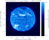 |
Fig. 5. Image of chromospheric H I Lyα intensity derived from the EIT 30.4 nm observation on 1997 October 8, in the same unit scale as the image given by Akinari (2008) and obtained by UVCS Lyα spectrometric measurements on the solar disc. |
4. Discussion of the results
4.1. Lyα line irradiance throughout the outer corona
The H I Lyα Carrington maps provide a representation of the daily non-uniform distribution of the chromospheric Lyα line intensity on the Sun, which is fundamental for an accurate determination of the solar wind outflow velocities. These maps were also used to compute the irradiance of the chromospheric Lyα radiation throughout the outer corona. Irradiance is the integral of the Doppler-shifted chromospheric intensity (or radiance) over the solid angle under which a coronal point subtends the solar disc, and gives the total amount of exciting radiation that incides on the scattering H I atoms in that point. It is not the unique factor responsible for the intensity of the resonantly scattered Lyα line in the corona, which also depends on the physical properties of the coronal particles. Measurements of the solar UV spectral irradiance were performed at a heliocentric distance of 1 AU by SOLSTICE/UARS. The instrument provided over about one decade (1991–2001) the daily mean solar spectrum from 115 to 425 nm with a spectral resolution of 1 nm. The SOLSTICE measurements can be exploited as a constraint on the irradiances derived from the Lyα Carrington maps. We compared the SOLSTICE irradiance at 121.6 nm with the irradiance computed at 1 AU from the mean intensity value over the portion of Carrington map that corresponds to the solar hemisphere that is visible from UARS (from −90° to +90° in longitude). Figure 6 shows that the Lyα irradiances obtained from the Carrington maps and SOLSTICE data agree very well throughout June 1997, with differences of about a few percent that are lower than the SOLSTICE accuracy (10%, see e.g. Lemaire et al. 2002).
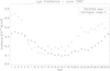 |
Fig. 6. Comparison of Lyα irradiances obtained from the constructed H I 121.6 nm Carrington maps (plus sign) and from the SOLSTICE measurements (open circle) in June 1997. |
Computations of the Lyα line irradiance in the outer corona, both on the plane of the sky (POS) and along the line of sight, have been performed for the first time here, taking into account the inhomogeneities of the chromospheric intensity distribution. A similar attempt was previously carried out only on the POS by Bemporad et al. (2003), who based their analysis on the calculation of the percentage of the solar disc area that is covered by active regions by means of MDI/SOHO images (Zayer et al. 1995). This alternative approach also provided good agreement with the SOLSTICE measurements and could be taken into consideration in the future. Figure 7 shows as an example the irradiance latitudinal profiles (solid lines) obtained in this work at projected heliocentric distances of 1.5 and 4.0 R⊙ on the POS by using the non-uniform intensity distribution in the Carrington map of June 7. The shape of the profiles agrees with the distribution of the brighter and darker features on the solar disc that we show in the top left panel of Fig. 4. Active regions appear to be gathered at the equatorial latitudes and mostly around the solar west limb (+90° longitude in the Carrington map), which means that they provide the higher irradiance values at the corresponding latitudes in the corona. Conversely, the illumination pattern of the coronal polar regions is obscured by the dark holes that are confined at the higher (in absolute value) latitudes. The same irradiance profiles were also obtained in the case of uniform-disc approximation (dashed lines), assuming a constant chromospheric intensity equal to the mean value over the entire Carrington map. A constant intensity obviously determines a constant irradiance profile at a given heliocentric distance. The comparison between the latitudinal profiles at a same altitude indicates that the assumption of uniform chromospheric radiation leads to an overestimated irradiance in a wide coronal area, including the poles and most of the mid-latitude regions, whereas the irradiance at the equatorial latitudes is underestimated. This is also confirmed by the plot reported in Fig. 8. For the four selected days of June 1997, it shows the radial profiles of the percentage ratio (Irru−Irrnu)/Irru averaged over coronal polar, mid-latitude, and equatorial regions, where Irru and Irrnu are the Lyα line irradiance values computed in the case of a uniform and non-uniform disc, respectively. We can note that the overestimated irradiance Irru reaches values that are up to 12–13% higher than Irrnu at the lower altitudes in the polar and mid-latitude regions. Close to the Sun, the solid angle subtended by the visible portion of the chromosphere at a given coronal point is significantly smaller than that of the entire solar disc, and the contribution of the darker polar features to the non-uniform illumination prevails. At higher heliocentric distances, the visible portion of the Sun converges to a full hemisphere. Equatorial active regions and dark polar holes contribute almost equally to the total illumination of the corona, providing irradiance values similar to those obtained in the case of a uniform-disc approximation. The opposite behaviour is visible in the coronal equatorial regions, where the exciting radiation from the brighter disc features dominates and the assumption of uniform chromospheric intensity leads to an underestimated irradiance from a maximum of 15% at 1.5 R⊙ down to 5% at 4.0 R⊙. The Carrington maps reported in Fig. 4 show a quite similar latitudinal distribution of the disc intensity for the four dates. This produces an equivalent illumination pattern and implies that the small departures in the radial profiles in Fig. 8 are mainly due to the differences in intensity values that were assumed in the uniform-disc approximation.
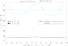 |
Fig. 7. Latitudinal profiles of the Lyα line irradiance at the projected heliocentric distances of 1.5 (cyan) and 4.0 R⊙ (purple) on the POS computed by using the non-uniform intensity distribution in the Carrington map of June 7 (solid lines) and assuming a uniform chromospheric intensity equal to the mean value over the Carrington map (dashed lines). |
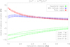 |
Fig. 8. Radial profiles between 1.5 and 4.0 R⊙ of the percentage ratio (Irru−Irrnu)/Irru averaged over equatorial (green), mid-latitude (blue), and polar (red) regions on 1997 June 7 (cross), 14 (open square), 18 (open diamond), and 21 (open upwards-pointing triangle). |
4.2. Solar wind H I outflow velocity maps
The intensity of the resonantly scattered H I Lyα line can be synthesised as described in Sect. 2 and Appendix A. Of the parameters to be used for the synthesis, the coronal electron density was derived from the coronagraphic VL images, the coronal electron temperature was obtained from standard temperature profiles taken from the literature, and the temperature of the scattering H I atoms was assumed to be isotropic and given by the map in Fig. 1. In addition, Carrington maps in the Lyα line were derived from analogous maps in the He II 30.4 nm line and were used to determine the intensity of the exciting chromospheric radiation, where the shape of the Lyα line profile follows Auchère (2005) and is assumed to be the same over the entire solar disc. This author numerically reproduced the line profile obtained by spectrometric Lyα measurements with SUMER/SOHO (Wilhelm et al. 1995) during the minimum phase of the solar magnetic activity cycle (see e.g. Lemaire et al. 2002). The expression of the Lyα line profile of Auchère (2005) is reported in Eq. (A.2).
Under these assumptions, the Lyα line intensity in the corona can be synthesised by means of Eq. (A.3). We used a numerical code to compute the synthetic intensity in the altitude range 1.5–4.0 R⊙, and adopted an improved version of the procedure used by Dolei et al. (2018) that also takes into account local variations of the exciting chromospheric radiation. The code initially assumes that the value of the solar wind outflow velocity (υw) is equal to zero, uses Eq. (A.3), and compares the result with the intensity given by the coronagraphic UV images. If the synthetic intensity turns out to be higher than that obtained from the UV observations, the code increases the wind velocity value in order to cause the intensity reduction that is determined by the Doppler dimming effect. The velocity tuning continues until the best match between synthetic and observed intensities is reached (see Dolei et al. 2018 for a more detailed description).
Solar wind H I outflow velocities were derived for the four selected days of June 1997. Figure 9 shows the daily 2D velocity maps in the outer corona obtained between 1.5 and 4.0 R⊙. The resulting velocities exhibit values that increase radially with altitude up to about 150–200 km s−1 in the equatorial regions and 400 km s−1 in the polar regions, according to the latitudinal distribution of slow and fast wind components, except for tiny wind streams at equatorial latitudes with high velocities (υw > 100 km s−1), which decrease between 1.5 and 2.5 R⊙. An interpretation of these unexpected coronal velocity features has been given by Dolei et al. (2018).
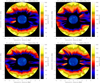 |
Fig. 9. 2D maps of the solar wind H I outflow velocity on the four selected days in June 1997. At the centre, we show the solar disc images in the H I Lyα line intensity derived from the relevant EIT 30.4 nm observations. |
The procedure for deriving the outflow velocity maps was also applied in the uniform-disc approximation, assuming for each day a constant chromospheric intensity equal to the mean value over the relevant Carrington map. In this case, Eq. (A.4) could be used, and a very short computational time is expected. Nevertheless, the code was not modified, and fictitious Carrington maps with constant intensity were used in order to exclude that different numerical computations determined different results. The H I velocity maps obtained in the uniform-disc approximation are not reported here. They exhibit morphologies similar to those of the maps in Fig. 9, but with significant departures that can be quantified by analysing Fig. 10. This map is related to the results of June 7 and shows the difference  , calculated in the outer coronal regions between 1.5 and 4.0 R⊙ on the POS, where
  and
and  are the outflow velocity values computed in the case of uniform and non-uniform disc, respectively. The difference
  corresponds to the outflow velocity variation depending on the adopted model of exciting chromospheric radiation. The map provides the radial and latitudinal dependence of this difference on the position of active regions and coronal holes at the solar limb, localised in the image of the chromospheric Lyα intensity reported at the centre. Above the polar regions, the velocities
  are higher than
  : the maximum departures, equal to about 50–60 km s−1, are obtained at the lower altitudes, where the coronal illumination pattern is mainly obscured by the large polar dark holes. As previously discussed by Auchère (2005), the Lyα intensity synthesised in the uniform-disc approximation is overestimated by about 15% with respect to the case of a non-uniform disc, particularly at lower altitudes in the polar coronal holes. Dolei et al. (2018) found that this overestimate can give rise to higher values of the resulting outflow velocities, up to about 50 km s−1 above the poles, which explains the higher velocity differences (yellow areas) at low altitudes in the polar regions shown in Fig. 10. At higher heliocentric distances above the poles, the differences
  decrease because bright and dark chromospheric features contribute nearly equally to the total illumination of the corona. Conversely, the velocities
  and
and  have quite similar values at equatorial latitudes throughout the entire 1.5–4.0 R⊙ altitude range, where the limited active regions contribute weakly to the coronal illumination pattern. This reflects on the values of the differences
  , which become slightly negative and suggest somewhat underestimated velocities in the assumption of uniform chromospheric radiation. Analogous considerations derive from the results obtained for the other selected days of June 1997.
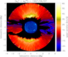 |
Fig. 10. 2D map of the difference |


5. Summary and conclusions
We studied solar wind dynamics in the outer coronal region by analysing coronagraphic UV and VL images. We selected data that were simultaneously acquired by space- and ground-based instruments over 1997 June 7, 14, 18, and 21, during the minimum phase between solar cycles 22 and 23. In particular, we used the H I Lyα synoptic spectrometric observations of UVCS/SOHO and the polarised brightness images of LASCO C2/SOHO and Mk3/MLSO.
The Lyα line emission in the solar corona is affected by the Doppler dimming effect, that is, the line intensity reduction that occurs as a consequence of the outward expansion of the solar plasma. The numerical computation of the Lyα line intensity was performed according to Eq. (1), by properly tuning the value of the solar wind outflow velocity in order to better reproduce the UV spectral observations. To synthesise the Lyα intensity, some physical properties of the solar corona were determined previously. In particular, the electron density was derived by the inversion technique of the VL polarised brightness, the electron temperature was obtained by an average of the standard values reported in the literature, and a temperature map of the H I atoms was reconstructed by considering very many Lyα spectral line data over a decade of UVCS observations at solar minimum. To compute the synthetic Lyα intensity, we also needed to determine the distribution of the exciting Lyα radiation over the solar chromosphere. We constructed Carrington rotation maps of the chromospheric Lyα intensity, centred at the location of the central meridian on the selected dates in June 1997. This provided a representation of the daily non-uniform distribution on the Sun. In lack of systematic full-disc Lyα observations, these maps were obtained from analogous maps in the He II 30.4 nm line and were then converted into H I 121.6 nm line emission by applying the correlation function established by Auchère (2005) that we report in Eq. (2). However, the comparison with UVCS disc measurements in the Lyα line, acquired in October 1997, showed that the conversion from He II 30.4 nm into H I 121.6 nm intensity could provide underestimated values in the polar coronal holes because He II data near the poles in the original Carrington maps are lacking. All these uncertainties should be considered in the evaluation of the resulting outflow velocities at the poles.
Irradiance values of the chromospheric Lyα radiation were computed throughout the outer coronal region, both using the non-uniform intensity distribution in the Carrington maps and assuming constant intensities equal to the mean values over the entire Carrington maps. In the first case, the resulting illumination pattern is in agreement with the expected distribution of the bright active regions, mostly gathered at the equatorial latitudes, and dark coronal holes, confined at the polar latitudes. Otherwise, the assumption of uniform chromospheric radiation leads to an overestimated irradiance in a wide coronal area including the poles and most of the mid-latitude regions, whereas underestimated irradiance values are obtained at the equatorial latitudes. Although we explicitly considered inhomogeneities in the chromospheric Lyα intensity, variations in shape of the line profile depending on the solar disc brightness features (up to 10%, see Lemaire et al. 2002) were neglected here. The actual shape of the incident profile is important for determining the Doppler dimming effect and should be also considered in a detailed study of solar wind dynamics.
Global maps of the solar wind H I outflow velocity were derived by iterative comparison between the observed and synthetic Lyα line intensity with the Doppler dimming technique. These maps provide a picture of the distribution of the outflowing coronal plasma, both in heliocentric distance and in latitude. In particular, over the minimum phase of the solar magnetic activity cycle, they exhibit a clear boundary between fast (polar) and slow (equatorial) solar wind regions. The procedure for deriving the outflow velocity maps was applied both in uniform and non-uniform radiation conditions. Significant differences in the polar coronal regions are present between the two cases, up to about 50–60 km s−1 closer to the Sun. Conversely, at progressively higher heliocentric distances, the portion of the solar surface that is visible from the corona tends to cover the full hemisphere, and the non-uniformly bright disc features can equally contribute to the illumination of the solar corona. This provides a radiation condition that is similar to the uniform-disc approximation.
In conclusion, we adopted a combination of different techniques to obtain 2D global maps of the solar wind H I outflow velocity in the outer coronal region by analysing narrow-band imaging in the UV Lyα spectral line, complemented by VL pB data. The Metis coronagraph (Antonucci et al. 2019), included in the scientific payload of the forthcoming Solar Orbiter mission (Müller et al. 2013, and in prep.), will provide this type of data. For the first time, it will acquire simultaneous coronagraphic images between 1.6 and 7.5 R⊙ in the UV H I Lyα line at 121.6 nm and broad-band (580–640 nm) VL polarised brightness, which will provide an unprecedented view of the solar wind acceleration regions. As for the exciting chromospheric Lyα line radiation, the Metis investigation will be supported by the full-disc images in the He II line emission at 30.4 nm, which will be provided almost simultaneously by the EUI Full Sun Imager (FSI), after applying the correlation function established by Auchère (2005). A valid constraint on the technique described in this work, and in particular, on the correlation function between the H I 121.6 nm and He II 30.4 nm line intensities, will be also provided by the measurements of chromospheric Lyα emission that will be acquired in a limited field of view by the High Resolution Imager (HRI) of EUI. In addition, direct observations of the polar regions during the out-of-ecliptic phases of the Solar Orbiter mission will provide He II line data near the poles, which are currently missing in the available Carrington maps (Benevolenskaya et al. 2001).
Acknowledgments
The authors acknowledge the support of the Italian Space Agency (ASI) to this work through contracts ASI/INAF No. I/013/12/0 and No. 2018-30-HH.0.
References
- Akinari, N. 2008, ApJ, 674, 1167 [NASA ADS] [CrossRef] [Google Scholar]
- Antonucci, E., Abbo, L., & Telloni, D. 2012, Space Sci. Rev., 172, 5 [NASA ADS] [CrossRef] [Google Scholar]
- Antonucci, E., Romoli, M., Fineschi, S., et al. 2019, A&A, in press, DOI: 10.1051/0004-6361/201935338 [Google Scholar]
- Auchère, F. 2005, ApJ, 622, 737 [NASA ADS] [CrossRef] [Google Scholar]
- Beckers, J. M., & Chipman, E. 1974, Sol. Phys., 34, 151 [NASA ADS] [CrossRef] [Google Scholar]
- Bemporad, A. 2017, ApJ, 846, 86 [NASA ADS] [CrossRef] [Google Scholar]
- Bemporad, A., Poletto, G., Suess, S. T., et al. 2003, ApJ, 593, 1146 [NASA ADS] [CrossRef] [Google Scholar]
- Benevolenskaya, E. E., Kosovichev, A. G., & Scherrer, P. H. 2001, ApJ, 554, 107 [Google Scholar]
- Bertaux, J.-L., Kyrölä, E., Quémerais, E., et al. 1995, Sol. Phys., 162, 403 [NASA ADS] [CrossRef] [Google Scholar]
- Bertaux, J.-L., Quémerais, E., Lallement, R., et al. 2000, Geophys. Res. Lett., 27, 1331 [NASA ADS] [CrossRef] [Google Scholar]
- Brueckner, G. E., Howard, R. A., Koomen, M. J., et al. 1995, Sol. Phys., 162, 357 [NASA ADS] [CrossRef] [Google Scholar]
- Cook, J. W., Newmark, J. S., Moses, J. D., et al. 1999, Proc. 8th SOHO Workshop, Plasma Dynamics and Diagnostics in the Solar Transition Region and Corona, ESA SP-446 (Noordwijk: ESA), 241 [Google Scholar]
- Cranmer, S. R., Kohl, J. L., Noci, G., et al. 1999, ApJ, 511, 481 [NASA ADS] [CrossRef] [Google Scholar]
- Curdt, W., Brekke, P., Feldman, U., et al. 2001, A&A, 375, 591 [NASA ADS] [CrossRef] [EDP Sciences] [Google Scholar]
- Delaboudinière, J.-P., Artzner, G. E., Brunaud, J., et al. 1995, Sol. Phys., 162, 291 [NASA ADS] [CrossRef] [Google Scholar]
- Dere, K. P., Moses, J. D., Delaboudinière, J.-P., et al. 2000, Sol. Phys., 195, 13 [NASA ADS] [CrossRef] [Google Scholar]
- Dolei, S., Spadaro, D., & Ventura, R. 2015, A&A, 577, A34 [NASA ADS] [CrossRef] [EDP Sciences] [Google Scholar]
- Dolei, S., Spadaro, D., & Ventura, R. 2016, A&A, 592, A137 [NASA ADS] [CrossRef] [EDP Sciences] [Google Scholar]
- Dolei, S., Susino, R., Sasso, C., et al. 2018, A&A, 612, A84 [NASA ADS] [CrossRef] [EDP Sciences] [Google Scholar]
- Domingo, V., Fleck, B., & Poland, A. I. 1995, Sol. Phys., 162, 1 [NASA ADS] [CrossRef] [Google Scholar]
- Dominique, M., Hochedez, J.-F., Schmutz, W., et al. 2013, Sol. Phys., 286, 21 [NASA ADS] [CrossRef] [Google Scholar]
- Fisher, R. R., Lee, R. H., MacQueen, R. M., & Poland, A. I. 1981, Appl. Opt., 20, 1094 [NASA ADS] [CrossRef] [Google Scholar]
- Gabriel, A. H. 1971, Sol. Phys., 21, 392 [NASA ADS] [CrossRef] [Google Scholar]
- Gibson, S. E., Fludra, A., Bagenal, F., et al. 1999, J. Geophys. Res., 104, 9691 [NASA ADS] [CrossRef] [Google Scholar]
- Gouttebroze, P., Lemaire, P., Vial, J.-C., & Artzner, G. 1978, ApJ, 225, 655 [NASA ADS] [CrossRef] [Google Scholar]
- Hayes, A. P., Vourlidas, A., & Howard, R. A. 2001, ApJ, 548, 1081 [NASA ADS] [CrossRef] [Google Scholar]
- Hyder, C. L., & Lytes, B. W. 1970, Sol. Phys., 14, 147 [NASA ADS] [Google Scholar]
- Kohl, J. L., Esser, R., Gardner, L. D., et al. 1995, Sol. Phys., 162, 313 [NASA ADS] [CrossRef] [Google Scholar]
- Kohl, J. L., Noci, G., Antonucci, E., et al. 1997, Sol. Phys., 175, 613 [NASA ADS] [CrossRef] [Google Scholar]
- Kohl, J. L., Noci, G., Cranmer, S. R., & Raymond, J. C. 2006, A&ARv, 13, 31 [NASA ADS] [CrossRef] [Google Scholar]
- Lemaire, P., Emerich, C., Vial, J. C., et al. 2002, in From Solar Min to Max: Half a Solar Cycle with SOHO, ESA SP-508, ed. A. Wilson (Noordwijk: ESA), 219 [Google Scholar]
- Lemaire, P., Vial, J.-C., Curdt, W., Schühle, U., & Wilhelm, K. 2015, A&A, 581, A26 [NASA ADS] [CrossRef] [EDP Sciences] [Google Scholar]
- Müller, D., Marsden, R. G., & St.Cyr, O. C. & Gilbert, H. R., 2013, Sol. Phys., 285, 25 [NASA ADS] [CrossRef] [Google Scholar]
- Noci, G., Kohl, J. L., & Withbroe, G. L. 1987, ApJ, 315, 706 [NASA ADS] [CrossRef] [Google Scholar]
- Noci, G., Kohl, J. L., Antonucci, E., et al. 1997a, in Fifth SOHO Workshop: The Corona and Solar Wind Near Minimum Activity, ESA SP-404, ed. A. Wilson (Noordwijk: ESA), 75 [Google Scholar]
- Noci, G., Kohl, J. L., Antonucci, E., et al. 1997b, Adv. Space Res., 20, 2219 [NASA ADS] [CrossRef] [Google Scholar]
- Raymond, J. C., Kohl, J. L., Noci, G., et al. 1997, Sol. Phys., 175, 645 [NASA ADS] [CrossRef] [Google Scholar]
- Rottman, G. J., & Woods, T. N. 1994, SPIE, 2266, 317 [NASA ADS] [Google Scholar]
- Spadaro, D., Susino, R., Ventura, R., Vourlidas, A., & Landi, E. 2007, A&A, 475, 707 [NASA ADS] [CrossRef] [EDP Sciences] [Google Scholar]
- Spadaro, D., Susino, R., Dolei, S., Ventura, R., & Antonucci, E. 2017, A&A, 603, A35 [NASA ADS] [CrossRef] [EDP Sciences] [Google Scholar]
- Susino, R., Ventura, R., Spadaro, D., Vourlidas, A., & Landi, E. 2008, A&A, 488, 303 [NASA ADS] [CrossRef] [EDP Sciences] [Google Scholar]
- Susino, R., Bemporad, A., Jejčič, S., & Heinzel, P. 2018, A&A, 617, A21 [NASA ADS] [CrossRef] [EDP Sciences] [Google Scholar]
- Van De Hulst, H. C. 1950, Bull. Astron. Inst. Neth., 410, 135 [NASA ADS] [Google Scholar]
- Vasquez, A. M., Van Ballegooijen, A. A., & Raymond, J. C. 2003, ApJ, 598, 1361 [NASA ADS] [CrossRef] [Google Scholar]
- Vourlidas, A., Klimchuk, J. A., Korendyke, C. M., et al. 2001, ApJ, 563, 374 [NASA ADS] [CrossRef] [Google Scholar]
- Wilhelm, K., Curdt, W., Marsch, E., et al. 1995, Sol. Phys., 162, 189 [NASA ADS] [CrossRef] [Google Scholar]
- Withbroe, G. L., Kohl, J. L., Weiser, H., & Munro, R. H. 1982, Space Sci. Rev., 33, 17 [NASA ADS] [CrossRef] [Google Scholar]
- Woods, T. N., Rottman, G., & Vest, R. 2005, Sol. Phys., 230, 345 [NASA ADS] [CrossRef] [Google Scholar]
- Zayer, I., Morrison, M., Pope, T., et al. 1995, GONG 1994. Helio- and Astro-Seismology from the Earth and Space, 76, 456 [NASA ADS] [Google Scholar]
Appendix A: Resonantly scattered Lyα line intensity
Equation (1) provides the functional form of the intensity of the resonantly scattered component of the coronal Lyα line. This equation contains integrals over x, Ω, λ′, and v. Because the solid angle is, in turn, dΩ = sin ϑ dϑ dφ, additional integrations over ϑ and φ have to be considered. Numerical solution and long computational time are expected when this expression is used to determine outflow velocities. However, under suitable approximations, different parts of Eq. (1) can be analytically solved, as explained below.
A.1. Velocity distribution of the scattering H I atoms
The shape of the absorption profile Φ is determined by the velocity distribution function of the scattering H I atoms in the corona. If this function follows the Maxwell-Boltzmann distribution, the integral over υ can be analytically computed. The scalar product υ ⋅ n′ in the Doppler shift term is equal to υw cos ϑ + u(n′), where  is the most probable velocity of the H I atoms in the direction n′, kB is the Boltzmann constant, and mHI is the atomic mass of hydrogen. From Eq. (1) we have
![$$ \begin{aligned} \mathcal{I} ({\boldsymbol{n}}) =&\frac{0.833\,h\,B_\mathrm{12} }{4\sqrt{\pi ^3}\lambda _\mathrm{0} }\displaystyle \int _{-\infty }^{+\infty }\!\!\!\!\!\!\!n_\mathrm{e} \,R_\mathrm{i} \,\mathrm{d} x\\&\times \displaystyle \int _{\vartheta }\displaystyle \int _{\varphi }\frac{11+3({\boldsymbol{n}}\cdot {\boldsymbol{n^\prime }})^2}{12}\sin \vartheta \,\mathrm{d} \vartheta \,\mathrm{d} \varphi \nonumber \\&\times \displaystyle \int _{-\infty }^{+\infty }\!\!\!\!\!\!\!\mathcal{J} (\lambda \prime ,{\boldsymbol{n^\prime }})\frac{1}{{ w}}\exp \left[-\left(\frac{\lambda \prime -\lambda _\mathrm{0} }{{ w}}-\frac{\lambda _\mathrm{0} \,\upsilon _{ w}}{c\,{ w}}\cos \vartheta \right)^2\right]\,\mathrm{d} \lambda \prime , \nonumber \end{aligned} $$](/articles/aa/full_html/2019/07/aa35048-19/aa35048-19-eq17.gif)
with w = λ0 u(n′)/c.
A.2. Multi-Gaussian chromospheric Lyα radiation profile
The analytical solution of the integral over λ′ can be derived assuming a multi-Gaussian normalised chromospheric profile. The solar disc Lyα profile is strongly non-Gaussian, with a reversal in the line core and extended wings (see e.g. Curdt et al. 2001; Gouttebroze et al. 1978). Auchère (2005) proposed the following expression of the profile, as the sum of three Gaussian components:
![$$ \begin{aligned} \mathcal{J} (\lambda \prime ,{\boldsymbol{n^\prime }})=\mathcal{J} ({\boldsymbol{n^\prime }})\displaystyle \sum _{i=1}^{3}\,\left\{ \frac{a_\mathrm{i} }{\sigma _\mathrm{i} \sqrt{\pi }}\exp \left[-\left(\frac{\lambda \prime -\lambda _\mathrm{0} -\delta \lambda \prime _\mathrm{i} }{\sigma _\mathrm{i} }\right)^2\right]\right\} \cdot \end{aligned} $$](/articles/aa/full_html/2019/07/aa35048-19/aa35048-19-eq18.gif)
The values of the parameters ai, σi, and  are reported in Table 1 of Auchère (2005). From Eqs. (A.1) and (A.2), we obtain
![$$ \begin{aligned} \mathcal{I} ({\boldsymbol{n}}) =&\frac{0.833\,h\,B_\mathrm{12} }{4\sqrt{\pi ^3}\lambda _\mathrm{0} }\displaystyle \int _{-\infty }^{+\infty }\!\!\!\!\!\!\!n_\mathrm{e} \,R_\mathrm{i} \,\mathrm{d} x\\&\times \displaystyle \int _{\vartheta }\displaystyle \int _{\varphi }\frac{11+3({\boldsymbol{n}}\cdot {\boldsymbol{n^\prime }})^2}{12}\,\mathcal{J} ({\boldsymbol{n^\prime }})\sin \vartheta \nonumber \\&\times \displaystyle \sum _{i=1}^{3}\left\{ \frac{a_\mathrm{i} }{\sqrt{{ w}^2+\sigma ^2_\mathrm{i} }}\exp \left[-\frac{\left(\delta \lambda \prime _\mathrm{i} -\frac{\lambda _\mathrm{0} }{c}\upsilon _{ { w}}\cos \vartheta \right)^2}{{ w}^2+\sigma ^2_\mathrm{i} }\right]\right\} \mathrm{d} \vartheta \,\mathrm{d} \varphi . \nonumber \end{aligned} $$](/articles/aa/full_html/2019/07/aa35048-19/aa35048-19-eq20.gif)
A.3. Isotropic H I temperature and uniform chromospheric Lyα radiation
In Eq. (A.3) the intensity 𝒥(n′) is a function of the incoming direction n′ determined by the angles ϑ and φ. When this intensity is assumed to be uniform on the solar disc, then 𝒥(n′) = 𝒥 can be brought out from the integrals. When it is also assumed that the velocity of the scattering H I atoms is the same in any direction, that is, u(n′) = u, then the quantity w is a constant that only depends on the value of the isotropic H I kinetic temperature. In these cases and considering that n ⋅ n′ = cos ϕ cos ϑ − sin ϕ cos φ sin ϑ, the integral over φ in Eq. (A.3) can be analytically solved, and we obtain
![$$ \begin{aligned} \mathcal{I} ({\boldsymbol{n}}) =&\frac{0.833\,h\,B_\mathrm{12} }{2\sqrt{\pi }\,\lambda _\mathrm{0} }\,\mathcal{J} \displaystyle \int _{-\infty }^{+\infty }\!\!\!\!\!\!\!n_\mathrm{e} \,R_\mathrm{i} \,\mathrm{d} x\\&\times \displaystyle \int _{\vartheta }\left[\frac{11+3\left(\cos ^2\phi \cos ^2\vartheta +\frac{1}{2}\sin ^2\phi \sin ^2\vartheta \right)}{12}\right]\sin \vartheta \nonumber \\&\times \displaystyle \sum _{i=1}^{3}\left\{ \frac{a_\mathrm{i} }{\sqrt{{ w}^2+\sigma ^2_\mathrm{i} }}\exp \left[-\frac{\left(\delta \lambda \prime _\mathrm{i} -\frac{\lambda _\mathrm{0} }{c}\upsilon _{ { w}}\cos \vartheta \right)^2}{{ w}^2+\sigma ^2_\mathrm{i} }\right]\right\} \mathrm{d} \vartheta , \nonumber \end{aligned} $$](/articles/aa/full_html/2019/07/aa35048-19/aa35048-19-eq21.gif)
where ϕ is the angle between the radial direction of the outflow velocity vector υ and the line of sight n.
In summary, the functional forms reported in these equations allow us to synthesise the intensity of the resonantly scattered Lyα line, taking into account a series of possible approximations, and to determine the solar wind outflow velocity by means of the Doppler dimming technique. It is worth noting that assuming these approximations significantly reduces the computational time, which makes this technique also useful for a quick-look data analysis of coronagraphic UV observations.
All Figures
|
Fig. 1. Reconstructed H I temperature map at solar minimum. |
| In the text | |
|
Fig. 2. Carrington rotation maps 1923 and 1924 in the He II 30.4 nm line. The intensity range extends from 2.3 to 335.6 W m−2 sr−1. |
| In the text | |
|
Fig. 3. Carrington rotation maps 1923 and 1924 in the H I Lyα line. The intensity range extends from 38.8 to 435.5 W m−2 sr−1. The vertical dashed white lines mark the location of the central meridian on 1997 June 7, 14, 18, and 21 from right to left, respectively. |
| In the text | |
|
Fig. 4. H I Lyα Carrington maps centred at the location of the central meridian on 1997 June 7, 14, 18, and 21, respectively. Coronal plasma outflowing on the POS is mainly illuminated by the solar disc regions around −90° longitude (east limb) and +90° longitude (west limb). |
| In the text | |
|
Fig. 5. Image of chromospheric H I Lyα intensity derived from the EIT 30.4 nm observation on 1997 October 8, in the same unit scale as the image given by Akinari (2008) and obtained by UVCS Lyα spectrometric measurements on the solar disc. |
| In the text | |
|
Fig. 6. Comparison of Lyα irradiances obtained from the constructed H I 121.6 nm Carrington maps (plus sign) and from the SOLSTICE measurements (open circle) in June 1997. |
| In the text | |
|
Fig. 7. Latitudinal profiles of the Lyα line irradiance at the projected heliocentric distances of 1.5 (cyan) and 4.0 R⊙ (purple) on the POS computed by using the non-uniform intensity distribution in the Carrington map of June 7 (solid lines) and assuming a uniform chromospheric intensity equal to the mean value over the Carrington map (dashed lines). |
| In the text | |
|
Fig. 8. Radial profiles between 1.5 and 4.0 R⊙ of the percentage ratio (Irru−Irrnu)/Irru averaged over equatorial (green), mid-latitude (blue), and polar (red) regions on 1997 June 7 (cross), 14 (open square), 18 (open diamond), and 21 (open upwards-pointing triangle). |
| In the text | |
|
Fig. 9. 2D maps of the solar wind H I outflow velocity on the four selected days in June 1997. At the centre, we show the solar disc images in the H I Lyα line intensity derived from the relevant EIT 30.4 nm observations. |
| In the text | |
|
Fig. 10. 2D map of the difference |
| In the text | |
Current usage metrics show cumulative count of Article Views (full-text article views including HTML views, PDF and ePub downloads, according to the available data) and Abstracts Views on Vision4Press platform.
Data correspond to usage on the plateform after 2015. The current usage metrics is available 48-96 hours after online publication and is updated daily on week days.
Initial download of the metrics may take a while.