| Issue |
A&A
Volume 624, April 2019
|
|
|---|---|---|
| Article Number | A32 | |
| Number of page(s) | 10 | |
| Section | Stellar structure and evolution | |
| DOI | https://doi.org/10.1051/0004-6361/201834706 | |
| Published online | 03 April 2019 | |
Variation of the magnetic field of the Ap star HD 50169 over its 29-year rotation period⋆
1
European Southern Observatory, Alonso de Cordova 3107, Vitacura, Santiago, Chile
e-mail: This email address is being protected from spambots. You need JavaScript enabled to view it.
2
Special Astrophysical Observatory, Russian Academy of Sciences, Nizhnii Arkhyz 369167, Russia
3
Institute of Astronomy of the Russian Academy of Sciences, 48 Pyatnitskaya St, 119017
Moscow, Russia
4
Leibniz-Institut für Astrophysik Potsdam (AIP), An der Sternwarte 16, 14482
Potsdam, Germany
5
Department of Physics & Astronomy, University of Western Ontario, 1151 Richmond Street, London, Ontario N6A 3K7, Canada
6
Armagh Observatory, College Hill, Armagh BT61 9DG, UK
7
European Southern Observatory, Karl-Schwarzschild-Str. 2, 85748
Garching bei München, Germany
Received:
22
November
2018
Accepted:
14
February
2019
Abstract
Context. The Ap stars that rotate extremely slowly, with periods of decades to centuries, represent one of the keys to the understanding of the processes leading to the differentiation of stellar rotation.
Aims. We characterise the variations of the magnetic field of the Ap star HD 50169 and derive constraints about its structure.
Methods. We combined published measurements of the mean longitudinal field ⟨Bz⟩ of HD 50169 with new determinations of this field moment from circular spectropolarimetry obtained at the 6m telescope BTA of the Special Astrophysical Observatory of the Russian Academy of Sciences. For the mean magnetic field modulus ⟨B⟩, literature data were complemented by the analysis of ESO spectra, both newly acquired and from the archive. Radial velocities were also obtained from these spectra.
Results. We present the first determination of the rotation period of HD 50169, Prot = 29.04 ± 0.82 yr. HD 50169 is currently the longest-period Ap star for which magnetic field measurements have been obtained over more than a full cycle. The variation curves of both ⟨Bz⟩ and ⟨B⟩ have a significant degree of anharmonicity, and there is a definite phase shift between their respective extrema. We confirm that HD 50169 is a wide spectroscopic binary, refine its orbital elements, and suggest that the secondary is probably a dwarf star of spectral type M.
Conclusions. The shapes and mutual phase shifts of the derived magnetic variation curves unquestionably indicate that the magnetic field of HD 50169 is not symmetric about an axis passing through its centre. Overall, HD 50169 appears similar to the bulk of the long-period Ap stars.
Key words: stars: individual: HD 50169 / stars: chemically peculiar / stars: rotation / stars: magnetic field / binaries: spectroscopic
Based on observations collected at the European Southern Observatory under ESO Programmes 62.L-0867, 64.L-0443, and 2100.D-5013; on observations collected at the 6-m telescope BTA of the Special Astrophysical Observatory of the Russian Academy of Sciences; and on data products from observations made with ESO Telescopes at the La Silla Paranal Observatory under programmes 68.D-0254, 74.C-0102, 75.C-0234, 76.C-0073, 79.C-0170, 80.C-0032, 81.C-0034, and 82.C-0308.
© ESO 2019
1. Introduction
One of the most intriguing properties of the Ap stars is their slow rotation, compared to the superficially normal main-sequence stars in the same temperature range. In recent years, it has emerged that several percent of the Ap stars have rotation periods exceeding one month, and that the longest rotation periods reach several centuries (Mathys 2017). Perhaps even more puzzling is the spread of the rotation periods of the Ap stars, as some of them are as short as 0.5 d. How period differentiation over at least five orders of magnitude is achieved in stars that are essentially at the same evolutionary stage remains to be fully explained. Spruit (2018) recently argued that it is impossible for Ap stars to achieve sufficient braking once they are formed, so that they must have acquired their slow rotation already during the accretion phase, through a magnetic connection between the accreting matter and the birth cloud. This is only the conclusion of the latest attempt to build up a theory that accounts for the observed distribution of the rotation periods of the Ap stars. Like all previous similar attempts, however, the possibility of critically testing this theory is strongly limited by the still very incomplete knowledge of the long-period end of that distribution.
In turn, this incompleteness arises in large part, but definitely not entirely, from the finite time base over which relevant data have been collected. The first determination of the rotation period of an Ap star (α2 CVn = HD 112413, Prot = 5.5 d) was achieved just over one century ago (Belopolsky 1913), and hardly more than 70 years have elapsed since the first detection of a magnetic field in such a star (78 Vir = HD 118022, Babcock 1947). CS Vir (=HD 125248) was the first star in which the periodicity of the variations of the magnetic field was established (Babcock 1951); the magnetic and spectral variations were found to have the same period. By the end of the decade, out of ∼70 Ap stars known to be magnetic, Babcock (1958) identified only 5 as showing definitely periodic magnetic variations. By that time, however, Deutsch (1956) had convincingly shown that the oblique rotator model (Stibbs 1950) could account for the observed magnetic, spectroscopic, and photometric variability of the Ap stars. Eventually, Preston (1970b) presented the definitive arguments supporting this model. The only remaining issue was how the few Ap stars with very long periods that were known at the time fit in the context of this model. This triggered increased interest in these stars. Preston (1970a) compiled a list of stars that might have long periods. He took advantage of the low v sin i of these stars to carry out a first systematic study of the mean magnetic field modulus, discovering five new stars with resolved magnetically split lines (in addition to the 4 that were previously known) and estimating “surface fields” (or upper limits) for 21 more (Preston 1971).
In other words, the dedicated investigation of the longest variation periods of Ap stars started less than 50 years ago. Highlights of the first two decades of this effort include the works of Wolff (1975), Hensberge et al. (1984), and Rice (1988). However, the overall picture remained patchy. Photoelectric photometry, the tool of choice for the determination of Ap star periods of up to several weeks, proved much less suited to the study of slower variations because of its limitations with respect to long-term stability and reproducibility. The discovery of new Ap stars with resolved magnetically split lines (Mathys 1990), and the realisation that there were many more such stars to be found (Mathys & Lanz 1992), triggered a systematic search and extensive follow-up monitoring to identify these stars and characterise their magnetic fields (Mathys et al. 1997; Mathys 2017). As a result, many new very slowly rotating stars were found.
The milestones identified above set upper limits to the time base over which magnetic field measurements of the Ap stars were obtained: ∼70 yr since the first magnetic stars were discovered, ∼50 yr since the interest of the stars with the longest periods was recognised, and ∼25 yr since stars with very long periods started to be discovered in statistically significant numbers. The majority of the longest period stars have only been identified more recently and observed for less than 25 years, so that their variations could not be fully characterised yet. Even for the long-period star that has been followed for the longest time, γ Equ (=HD 201601), a full rotation cycle has not been covered by the observations that have been acquired so far, however. This star is one of the first half-dozen Ap stars in which a magnetic field was detected, for which the first longitudinal field measurements were obtained in 1946 (Babcock 1948). The most recent estimate of the lowest plausible value of the period for this star places it at 97 yr (Bychkov et al. 2016), and the possibility that it is even longer cannot be ruled out. Existing ⟨Bz⟩ measurements still cover at most only ∼70% of the full rotation cycle of this star. Incidentally, the first measurement of its mean magnetic field modulus from the magnetic splitting of a spectral line was obtained less than 30 years ago (Mathys 1990), so that the current coverage of the ⟨B⟩ variation curve is less than one-third of the rotation period. In most cases, the phase coverage achieved so far is even more incomplete. For instance, Hubrig et al. (2018) recently proposed a tentative value of 188 yr for the rotation period of HD 101065 (Przybylski’s star) by extrapolation of magnetic observations that would span less than one-fourth of a rotation cycle.
These considerations illustrate the fundamental limitations to our ability to characterise the most slowly rotating Ap stars and emphasise the value of any new addition to the small group of very long period stars whose magnetic variations have been observed over a full rotation cycle. Prior to this study, the five Ap stars with the longest periods for which complete magnetic variation curves had been obtained were, in order of decreasing period length, HD 9996 (=HR 465, Prot = 7937 d, Metlova et al. 2014), HD 94660 (=HR 4263, Prot = 2800 d, Mathys 2017), HD 187474 (=HR 7552, Prot = 2345 d, Mathys 1991), HD 59435 (=BD −8 1937, Prot = 1360 d, Wade et al. 1999), and HD 18078 (=BD +55 726, Prot = 1358 d, Mathys et al. 2016).
HD 50169 (= BD −1 1414) is an A3p SrCrEu star (Renson & Manfroid 2009) in which the presence of a strong magnetic field was first reported by Babcock (1958) from spectroscopic observations in circular polarisation. Preston (1971) noted its very low v sin i (< 10 km s−1) and obtained a first estimate of its mean magnetic field modulus (which he referred to as mean surface magnetic field), 5.6 kG, from consideration of the differential broadening of spectral lines with Zeeman patterns of different widths. Following the discovery that the Fe II λ 6149.2 line is resolved into its magnetically split components in the spectrum of HD 50169 (Mathys & Lanz 1992), more magnetic measurements started to be acquired, both of the mean longitudinal field ⟨Bz⟩ (Mathys & Hubrig 1997; Romanyuk et al. 2014; Mathys 2017) and of the mean field modulus ⟨B⟩ (Mathys et al. 1997; Mathys 2017). Combining all the available measurements, Mathys (2017) concluded that the rotation period of the star must be much longer than 7.5 yr. However, he also argued that this period should likely be shorter than 40 yr.
Here we present additional determinations of ⟨Bz⟩ and ⟨B⟩, based on both new dedicated observations and archive spectra, and we use them to derive for the first time the value of the rotation period of HD 50169. The observational data and their analysis are described in Sect. 2, and the determination of the stellar rotation period is presented in Sect. 3. In Sect. 4 we derive constraints on the geometrical structure of the magnetic field, and in Sect. 5 we refine the determination of the orbital elements of the HD 50169 binary system. Finally, we draw conclusions and discuss future prospects (Sect. 6).
2. Observations and data analysis
2.1. Mean magnetic field modulus
The mean magnetic field modulus ⟨B⟩ is the average over the visible stellar disc of the modulus of the field vector, weighted by the local emergent line intensity. The following published measurements of this field moment were used in this study:
-
thirteen measurements from Mathys et al. (1997),
-
and eight measurements from Mathys (2017).
These measurements were obtained with four different instrumental configurations. For the sake of simplicity, we use the same symbols as Mathys (2017) to identify these configurations in Fig. 2.
Here, we present new ⟨B⟩ data at additional epochs from the analysis of the following high-resolution spectra recorded in natural light:
-
Two spectra recorded with the Very Long Camera (VLC) of the ESO Coudé Echelle Spectrograph (CES) fed by the ESO 3.6 m telescope (Dall 2005). This configuration is quite different from those used by Mathys et al. (1997) and Mathys (2017), but the reduction process was very similar to the one applied for other fibre-fed CES configurations in these previous studies (see Sect. 3 of Mathys et al. 1997 for details).
-
Twenty-three spectra recorded with the High Accuracy Radial velocity Planet Searcher (HARPS) fed by the ESO 3.6 m telescope, retrieved from the ESO Archive.
-
Three spectra recorded with the Ultraviolet and Visible Echelle Spectrograph (UVES) fed by Unit Telescope 2 (UT2) of the ESO Very Large Telescope (VLT). One of these spectra was retrieved from the ESO Archive, the other two were purpose-made DDT observations intended to constrain the strength of the mean magnetic field modulus around the phase of its minimum.
For the HARPS and UVES observations, we used science-grade pipeline-processed data available from the ESO Archive. The only additional processing that we carried out was a continuum normalisation of the region (∼100 Å wide) surrounding the Fe II λ 6149.2 diagnostic line.
This line is resolved in its two magnetically split components in all the spectra that we analysed. We measured the wavelength separation of the components to determine the mean magnetic field modulus ⟨B⟩ at the corresponding epochs, by application of the formula
 (1)
(1)
In this equation, λr and λb are the wavelengths of the red and blue split line components, respectively; g is the Landé factor of the split level of the transition (g = 2.70; Sugar & Corliss 1985);  , with k = 4.67 10−13 Å−1 G−1; and λ0=6149.258 Å is the nominal wavelength of the considered transition.
There is no reason to expect the uncertainty of the new determinations of ⟨B⟩ presented here to be significantly different from that of the previous measurements of Mathys et al. (1997) and Mathys (2017). We show in Sect. 3 that the scatter of the measurements about the variation curve of the mean magnetic field modulus is fully consistent with this adopted value of the uncertainty, 30 G. Incidentally, the ⟨B⟩ measurements in HD 50169 are among the most precise that can be obtained for any Ap star with resolved magnetically split lines because the split components of the Fe II λ 6149.2 line are among the sharpest, best resolved, and least blended of all, as is shown in Figs. 2–4 of Mathys et al. (1997).
The 49 values of the mean magnetic field modulus obtained in that way are presented in Table A.1. For convenience, this table also includes the previously published measurements. The columns give, in order, the Julian Date of the observation, the value ⟨B⟩ of the mean magnetic field modulus, the heliocentric radial velocity, and the source of the measurement. We note that the radial velocities determined by Mathys et al. (1997) were published by Mathys (2017). For the new determinations from this paper, the instrument that was used is specified; for published measurements, this information is available in the cited reference. The date that is given is the Heliocentric Julian Date (or Barycentric, for the HARPS observations) of mid-exposure, except for the two measurements based on CES VLC spectra, for which the headers were incomplete. For these two spectra, the listed mid-exposure time is accurate to the minute; its uncertainty does not have any significant effect on this study because the timescales involved are much longer. The radial velocity could not be determined for the first observation listed in this table owing to the lack of appropriate calibration. As mentioned elsewhere, the estimated uncertainties of the field modulus and radial velocity values are 30 G and 1 km s−1.
2.2. Mean longitudinal magnetic field
The mean longitudinal magnetic field ⟨Bz⟩ is the average over the visible hemisphere of the component of the magnetic vector along the line of sight, weighted by the local emergent line intensity. The following published measurements of this field moment were used in this study:
-
six measurements from Babcock (1958),
-
one measurement from Mathys & Hubrig (1997),
-
one measurement from Romanyuk et al. (2014),
-
and eight measurements from Mathys (2017).
All these measurements were carried out through the analysis of medium to high spectral resolution observations of metal lines in circular polarisation. Here they are complemented by additional ⟨Bz⟩ determinations obtained from observations of the same type, that is, spectra of HD 50169 recorded at R ≃ 14 500 in both circular polarisations with the Main Stellar Spectrograph of the 6 m telescope BTA of the Special Astrophysical Observatory, on 23 nights spread from December 2002 to February 2018. This is the same configuration as used by Romanyuk et al. (2014). The instrumental configuration and the data reduction procedure are as described in detail in this reference.
The mean longitudinal magnetic field was determined from the wavelength shifts of a sample of spectral lines between the two circular polarisations in each of these spectra by application of the formula
 (2)
(2)
where λR (resp. λL) is the wavelength of the centre of gravity of the line in right (left) circular polarisation and  is the effective Landé factor of the transition. ⟨Bz⟩ is determined through a least-squares fit of the measured values of λR − λL by a function of the form given above. The standard error σz that is derived from that least-squares analysis is used as an estimate of the uncertainty affecting the obtained value of ⟨Bz⟩.
The values of the mean longitudinal field obtained in that way are presented in Table A.2. For convenience, this table also includes the previously published measurements. The columns give, in order, the Julian Date of the observation, the value ⟨Bz⟩ of the mean longitudinal magnetic field and its uncertainty σz, and the source of the measurement. The accuracy of the date of observation is variable, ranging from the Heliocentric Julian Date of mid-exposure (Mathys & Hubrig 1997; Mathys 2017) to the mere date of observation, without any time specification (Babcock 1958). The associated phase uncertainty is only 10−5, which is completely negligible. In total, 39 ⟨Bz⟩ measurements are listed in Table A.2.
2.3. Radial velocities
Following Mathys (2017), we computed the unpolarised wavelength λI of the Fe IIλ 6149.2 line by averaging the wavelengths of its blue and red split components as measured for the determination of the mean magnetic field modulus, as follows:
 (3)
(3)
Then, the wavelength difference λI − λ0 was converted into a radial velocity value in the standard manner. The notations Wλ, b and Wλ, r refer to the equivalent widths of the measured parts of each line component. For more details, see Mathys (2017).
We applied this approach to all the additional high-resolution spectra recorded in natural light that we used to measure ⟨B⟩. The arguments presented by Mathys (2017) in support of the validity of this procedure are further strengthened by the consideration that the CES VLC, UVES, and HARPS are instruments (or instrumental configurations) that were designed to optimise radial velocity determinations for exoplanet searches and studies.
The new radial velocity measurements of this study are listed in Table A.1. We adopt for them the same uncertainty as for the similar measurements of Mathys (2017). This is somewhat arbitrary, but it seems justified since we did not take any particular care to optimise the radial velocity determinations, and the scatter of the new measurements about the revised orbital solution presented in Sect. 5 is of the same order as the scatter of the data from Mathys (2017).
3. Magnetic variability and rotation period
To determine the rotation period of HD 50169, we fitted the measurements of its mean longitudinal magnetic field by either a cosine wave or by the superposition of a cosine wave and of its first harmonic, progressively varying the period of these waves in search of the value of the period that minimises the reduced χ2 of the fit. These fits are weighted by the inverse of the square of the uncertainties of the individual measurements. Through this procedure, we concluded unambiguously that the rotation period of the star must be of the order of 10 800 d.
The usage of the procedure described above is justified by the well-documented observation that the variation curves of the magnetic field moments of Ap stars often closely resemble a cosine wave or the superposition of a cosine wave and of its first harmonic (e.g. Mathys 2017, and references therein). However, there is no physical reason why the variation curve of either ⟨Bz⟩ or ⟨B⟩ should have exactly such a shape. The complexity of the geometrical structure of the Ap star magnetic fields (a prominent example is 53 Cam = HD 65339, as shown by Kochukhov et al. 2004) implies that when sufficiently precise determinations of a field moment with good enough phase sampling are available (neither of which is fulfilled by the ⟨B⟩ measurements of HD 65339 of Mathys 2017), the actual variation curve of this field moment must show significant deviations from the simple mathematical approximations used here. This in turn implies that the estimate of the rotation period that is derived by fitting such a simple mathematical curve to the observational data must be critically assessed for fine adjustment and determination of its uncertainty.
The time elapsed between Babcock’s (1958) first determination of the mean longitudinal magnetic field of HD 50169 and our most recent spectropolarimetric observation of the star is 23 500 d, or ∼2.2 rotation periods. This provides a very sensitive approach to refine the determination of the period and to estimate its uncertainty. By plotting a phase diagram of the ⟨Bz⟩ measurements for a series of tentative values of the period around the one suggested by the periodogram, one can visually identify the period value that minimises the phase shifts between field determinations from different rotation cycles, and constrain the range around that value for which those phase shifts remain reasonably small. More specifically, in the present case, the ascending branch of the ⟨Bz⟩ variation curve proves particularly well suited to the application of this method: the measurements from Babcock (1958; red crosses) and our ⟨Bz⟩ determinations from 6m telescope observations (salmon-coloured filled squares) should remain aligned along the same line, without significant systematic phase shift of one set with respect to the other. Critically, the accuracy of the period determination carried out in this manner only depends on the reproducibility of the variation curve from one cycle to the next, not on its exact shape.
Admittedly, ⟨Bz⟩ determinations obtained with different instruments and by application of different data analysis methods are known to show frequently systematic differences, whose existence between the two sets of data of interest cannot definitely be ruled out. However, previous studies indicate that in general, for Ap stars with fairly sharp spectral lines, there are at most minor systematic differences between the longitudinal field values determined, through application of the metal line spectropolarimetric technique, by Babcock (from observations obtained with the Mount Wilson 100-inch and Palomar 200-inch coudé spectrographs), by Mathys and collaborators (from ESO CASPEC spectra), and by Romanyuk and collaborators (with the Main Stellar Spectrograph of the 6 m telescope BTA of the Special Astrophysical Observatory). Assuming that the ⟨Bz⟩ data sets that we combine here are indeed mutually consistent within their formal precision, we determine the following best value of the rotation period of HD 50169:
 (4)
(4)
The phase variation curve of ⟨Bz⟩ for this value of the period is shown in Fig. 1. We note the consistent behaviour of the measurements of Babcock and of Romanyuk’s group on the ascending branch between phases 0.1 and 0.5. The estimated uncertainty on the period factors in possible systematic shifts between the measurement sets from the different groups that are at most of the same order of magnitude as the formal errors of these measurements. That is, we regard as unacceptably long or unacceptably short period values for which in the phase diagram, within a given phase interval, a set of ⟨Bz⟩ data obtained by one of the groups is systematically offset with respect to the measurements by another group, performed in another rotation cycle, by an amount that significantly exceeds the uncertainties of the individual ⟨Bz⟩ determinations. Admittedly, there is a certain degree of arbitrariness involved in this procedure, not only because it is based on a visual inspection of the variation curves, but also, more critically, because it relies on the assumption that the systematic differences between measurements obtained by different groups with different instruments do not exceed the random errors affecting these measurements. This assumption is borne out by our experience of the consistency of the ⟨Bz⟩ measurements by the three groups in question in other stars. That we cannot know for sure whether for HD 50169 there are systematic differences between the measurements of the various groups and how large these differences are implies that we cannot either determine in a fully objective and unambiguous way the uncertainty affecting the derived value of the period. The 300 d value that we adopt for this uncertainty is our best educated estimate, significantly higher than the uncertainty derived from a formal fit, 88 d, which we regard as too low according to the arguments given above. Only the acquisition of additional measurements over a large portion of the next rotation cycle (more than a decade) will allow the determination of the period and of its uncertainty to be further improved.
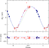 |
Fig. 1. Upper panel: mean longitudinal magnetic field of HD 50169 against rotation phase. The different symbols identify the source and/or instrumental configuration from which the ⟨Bz⟩ value was obtained, as follows: crosses (red): Babcock (1958); filled triangle (violet): Mathys & Hubrig (1997); filled circles (dark blue): Mathys (2017); filled squares (salmon): Romanyuk et al. (2014), and new measurements of spectra obtained with the Main Stellar Spectrograph of the 6 m telescope BTA of the Special Astrophysical Observatory. The long-dashed line (blue) is the best fit of the observations by a cosine wave and its first harmonic, see Eq. (5). The short-dashed line (green) corresponds to the superposition of low-order multipoles discussed in Sect. 4. Lower panel: differences O − C between the individual ⟨Bz⟩ measurements and the best-fit curve against rotation phase. The dotted lines (blue) correspond to ±1 rms deviation of the observational data about the fit (red dashed line). The symbols are the same as in the upper panel. |
The 10 600 d period value is also consistent with the observed behaviour of the mean magnetic field modulus. Our measurements of this field moment cover a shorter time span, 9856 d. They definitely rule out a period shorter than this time span, however. The phase diagram of the ⟨B⟩ variation for a period of 10 600 d is shown in Fig. 2. The way in which the measurement points line up along a smooth curve, with almost no scatter at all, is remarkable. It is fully consistent with the estimated error of the ⟨B⟩ values. The error bars are plotted in the figure, but because their size does not significantly exceed that of the symbols, they can hardly be distinguished.
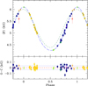 |
Fig. 2. Upper panel: mean magnetic field modulus of HD 50169 against rotation phase. The different symbols identify the source and/or instrumental configuration from which the ⟨B⟩ value was obtained, as follows: filled circles (dark blue): CAT + CES LC; open circles (steel blue): CAT + CES SC; filled hexagon (sea green): 3.6 m + CES LC; filled triangle (violet): CFHT + Gecko (all previous from Mathys et al. 1997; Mathys 2017); five-pointed open stars (orange): 3.6 m + CES VLC; four-pointed open stars (light green): UT2 + UVES; filled pentagons (yellow): 3.6 m + HARPS; filled square (salmon): Preston (1971). The long-dashed line (blue) is the best fit of the observations by a cosine wave and its first harmonic, see Eq. (6). The short-dashed line (green) corresponds to the superposition of low-order multipoles discussed in Sect. 4. Lower panel: differences O − C between the individual ⟨B⟩ measurements and the best-fit curve, against rotation phase. The dotted lines (blue) correspond to ±1 rms deviation of the observational data about the fit (red dashed line). The symbols are the same as in the upper panel. |
Moreover, agreement between the field values obtained with the different instrumental configurations is excellent. We do not find any systematic instrumental effects such as those that have occasionally affected previous measurements (e.g. Sect. 6 of Mathys et al. 1997). In particular, as we used HARPS and UVES spectra for the first time for ⟨B⟩ determinations, the good agreement of the resulting values with those obtained with instruments that we used in the past, such as the CES, is noteworthy. It strengthens our confidence that the mean magnetic field modulus measurements that we obtain using a large number of different instruments are free from any significant systematic errors of instrumental origin.
As our ⟨B⟩ measurements do not yet cover a full rotation cycle, we are not able to use the phase overlap between consecutive periods to constrain the value of the period, contrary to what we did for the mean longitudinal field. However, these measurements provide the following useful indication. For values of the rotation period comprised between 10 300 and 10 900 d (i.e. the uncertainty range set from the longitudinal field analysis), the ⟨B⟩ variations can be fitted well by a cosine curve and its first harmonic. This is quite similar to the behaviour observed in the vast majority of the Ap stars with resolved magnetically split lines. For instance, none of the stars analysed by Mathys (2017) for which sufficient phase coverage of the ⟨B⟩ measurements was achieved shows significant deviations from the superposition of a cosine wave and its first harmonic in the variations of this field moment. By contrast, if we attempt to fit the variations of the mean magnetic field modulus of HD 50169 with a period significantly outside the range 10 300–10 900 d, more harmonics become required in order for the fitted curve to match the observations.
Admittedly, we cannot definitely rule out the possibility of an unusual structure of the magnetic field of HD 50169, but this improbable coincidence appears all the less plausible since the resolved magnetically split components of the Fe II λ 6149.2 line in this star are particularly sharp and clean, while increased complexity in the geometrical structure of the magnetic field tends to manifest itself by distortions of the split line components, as was found in a recent study of HD 18078 (Mathys et al. 2016), for instance.
As we noted in the introduction, Preston (1971) was the first to obtain an estimate of the mean magnetic field modulus of HD 50169: 5.6 kG, derived from consideration of the differential broadening of spectral lines having Zeeman patterns of different widths. We retrieved the Julian Date of this observation from Adelman (1973), as the same spectrum was used for detailed abundance analysis. The representative point of Preston’s field determination appears as a salmon-coloured filled square in Fig. 2.
The uncertainty of this determination is difficult to assess. The most meaningful comparison between the field values derived by Preston (1971) through application of his Eq. (3) and the ⟨B⟩ determinations of Mathys (2017), based on the splitting of the Fe II λ 6149.2 doublet, is for those stars for which the mean field modulus only shows small, almost insignificant variations, such as HD 2453, HD 137949, and HD 192678. For these stars, the estimates of Preston (1971) and the measurements of Mathys (2017) are in excellent agreement, within ∼100 G of each other. The comparison is less straightforward when the field modulus shows definite variability with phase, but at least for some stars (e.g. HD 12288 or HD 188041), the agreement between the values that were derived from line broadening by Preston (1971) and those that Mathys (2017) obtained from consideration of the wavelength separation of split line components, seems somewhat poorer. The error bar on ⟨B⟩ that we adopted for the data point from Preston (1971) in Fig. 2, ±200 G, is only tentative, and it may well underestimate the actual uncertainty of the field values reported in this reference. Even with this “optimistic” accuracy, however, the magnetic field strength estimated nearly 50 years ago by Preston (1971) is consistent with the value of the rotation period that we derived above.
With Prot = 10 600 d, HD 50169 becomes the longest-period Ap star for which magnetic field measurements have been obtained over more than a full rotation cycle. At 29.04 yr, its period is considerably longer than the next longest one, 21.75 yr for HD 9996. Furthermore, with respect to the latter, HD 50169 presents the advantage of showing resolved magnetically split lines throughout its whole rotation cycle, so that its mean magnetic field modulus can be exactly determined even around the phase of its minimum and, as a consequence, the structure of the field can be better constrained.
4. Magnetic field characterisation
The observed variations of both the mean longitudinal magnetic field and the mean magnetic field modulus of HD 50169 can be well represented by the superposition of a cosine wave and of its first harmonic. The best least-squares fit solutions for Prot = 10 600 d are
![Mathematical equation: $$ \begin{aligned} \langle B_z\rangle (\phi )&=(253\pm 30)\nonumber \\&\;\;+(1566\pm 50)\,\cos \{2\pi \,[\phi -(0.583\pm 0.005)]\}\nonumber \\&\;\;+(290\pm 44)\,\cos \{2\pi \,[2\phi -(0.651\pm 0.027)]\}\nonumber \\&(\nu =34,\ \chi ^2/\nu =9.8),\end{aligned} $$](/articles/aa/full_html/2019/04/aa34706-18/aa34706-18-eq7.gif) (5)
(5)
![Mathematical equation: $$ \begin{aligned} \langle B\rangle (\phi )&=(5076\pm 10)\nonumber \\&\;\;+(922\pm 15)\,\cos \{2\pi \,[\phi -(0.004\pm 0.001)]\}\nonumber \\&\;\;+(107\pm 10)\,\cos \{2\pi \,[2\phi -(0.988\pm 0.017)]\}\nonumber \\&(\nu =44,\ \chi ^2/\nu =1.4), \end{aligned} $$](/articles/aa/full_html/2019/04/aa34706-18/aa34706-18-eq8.gif) (6)
(6)
where the field strengths are expressed in Gauss, ϕ = (HJD − HJD0)/Prot (mod 1) and the adopted value of HJD0 = 2441600.0 corresponds to a maximum of the mean magnetic field modulus; ν is the number of degrees of freedom, and χ2/ν, the reduced χ2 of the fit. The fitted curves are shown in Figs. 1 and 2; the O − C differences between the individual measurements and these curves are also illustrated. The ⟨B⟩ estimate of Preston (1971) was not taken into account for computation of the best fit. Its inclusion would only have affected the derived fit parameters insignificantly. The quality of the mean longitudinal magnetic field measurement on JD 2435765 is also debatable, as it appears to be a definite outlier. In the absence of any comment from Babcock (1958) about it, we included it in the ⟨Bz⟩ fit. Omitting it would not have yielded significantly different fit parameters, but the reduced χ2 would have been decreased from 9.8 to 6.3 (for 33 degrees of freedom). That this value is still rather high may indicate that the uncertainty of some of the measurements is slightly underestimated, that there are some (small) systematic differences between the measurements of the different groups, or that the actual shape of the ⟨Bz⟩ variation curve departs somewhat from the superposition of a cosine wave and its first harmonic, or some combination of these effects. This further strengthens our conviction that our conservative approach for the determination of the rotation period and of its uncertainty, based on the visual inspection of the consistency of measurements obtained at similar phases in different cycles and making allowance for unidentified (small) systematic errors, is warranted.
Within the estimated ±300 d uncertainty in the derived value of the rotation period, the ⟨B⟩ variation curve can be more or less stretched, but its general shape remains unchanged, mostly symmetrical about the phases of both its maximum (ϕM, max = 0.0) and its minimum (ϕM, min = 0.5). The magnetic minimum is somewhat broader and shallower than the maximum, as is frequently the case (Mathys 2017).
Because the mean longitudinal field measurements span more than two rotation cycles, the ⟨Bz⟩ variation curve is more sensitive to the length of the rotation period. In particular, depending on the exact value of this period, the phases of the extrema of ⟨Bz⟩ may be more or less shifted with respect to those of ⟨B⟩, and the ⟨Bz⟩ variation curve may show more or less pronounced (although never large) departures from symmetry about those phases. Regardless, the main features of the variations of the longitudinal field are quite definite: the phases of the extrema of ⟨Bz⟩ lag significantly behind those of ⟨B⟩, by a (period-dependent) amount close to 0.1 rotation cycle, and the ⟨B⟩ maximum occurs close to the negative extremum of ⟨Bz⟩, indicating that the magnetic field is stronger in the vicinity of the negative pole of the star than around the positive pole. The positive extremum of the longitudinal field is broader and shallower than the negative one, mirroring the above-mentioned difference between the minimum and the maximum of the ⟨B⟩ curve.
Simple parametrised magnetic field models of the distribution of magnetic flux over the stellar surface are frequently fitted to magnetic moment curves such as those of Figs. 1 and 2 in order to obtain a crude idea of the large-scale magnetic field structure of a star. These models, typically requiring only four or five parameters, certainly do not provide realistic details of the distribution of magnetic flux over the surface of the star, but they do allow us to estimate such interesting geometric parameters as the inclination i of the rotation axis to the line of sight, and the obliquity β of the magnetic axis (supposing that the field is nearly enough axisymmetric to have such an axis) to the rotation axis.
Amongst the simplest of such models is an expansion of the surface field in low-order axisymmetric multipoles (Stibbs 1950), using only the first two or three terms, for example using collinear dipole, quadrupole, and octupole (Landstreet 1988). Such models can usually be found, which fit the available magnetic moment measurements reasonably well (e.g. Landstreet & Mathys 2000). When such models are fit to a sample of magnetic Ap stars, a distinctive feature generally found is that the dipole component is almost always a major contributor to the expansion, while the importance of the higher terms is quite variable. A basic symptom of an important dipole component is that the highest ratio of |⟨Bz⟩/⟨B⟩| is of the order of 0.3. This is the case for HD 50169.
However, for this star it is obvious that the field distribution is not axisymmetric. An axisymmetric field distribution has the property that there are two phases, separated by 0.5 phase, through which all the field moment curves are reflectionally symmetric. The phase shift between the extrema of the ⟨Bz⟩ and ⟨B⟩ curves guarantees that there are no such phase pairs. Hence we must look for a simple field geometry that lacks axisymmetry.
In principle, if we allow enough free parameters (e.g. by taking an expansion in dipole, quadrupole, and octupole, all independently orientated with respect to the stellar rotation axis), we could probably fit the details of the observed field moment curves quite accurately, but also quite possibly non-uniquely. Instead, we look for a simple single parameter that we could add to the usual three coaxial multipole components and that reproduces approximately the phase shift between the extrema, without trying to fit all details of the (extremely well-defined) field moment curves.
A simple alteration to the usual axisymmetric multipole model that breaks the axisymmetry of the field model, and is easy to program, is to introduce a gradient in field strength in the direction normal to the plane containing the rotation and multipole axes. For example, taking a Cartesian coordinate system with the plane of the rotation and multipole axes as the x − z plane, we can simply multiply all field strengths at a given y–distance from the x − z plane by a factor 1 + Ay, where A < 1 is a single new parameter. This choice preserves div B = 0, while making the field somewhat stronger in one magnetic hemisphere than in the other. This choice also is found to lead to a shift in the relative extrema of one moment curve relative to the other that is approximately proportional to A.
Using a simple FORTRAN program that computes the field moments of a given field distribution, and searches for the multipole parameter values that agree best with a set of samples of the moments at various phases, we find that the best parameter values are i = 40°, β = 92° (note that i and β may be exchanged with no change in the predicted curves), Bdipole = −6930 G, Bquadrupole = −2490 G, Boctupole = +2880 G, and A = 0.14. Figures 1 and 2 show that the model computed with these parameters fits the observed moments fairly well, and in particular, it does produce about the observed phase shift between the extrema. As expected, the dipole is the dominating component of the field structure, but an asymmetry such as that introduced by A ≠ 0 is essential for the phase shift.
5. Binarity
Mathys et al. (1997) were the first to report the variability of the radial velocity of HD 50169. They suggested that the star could be a binary. This suspicion was supported by independent, contemporaneous radial velocity measurements from Carrier et al. (2002). Combining the latter with an extensive set of data built up as a by-product of his systematic study of the magnetic field of the star, Mathys (2017) computed for the first time the orbital elements of this binary. With the addition of the new radial velocity measurements obtained as part of the present study, the time base is increased by a factor of 3.6, albeit with a less dense sampling. This enables us to refine considerably the definition of most orbital elements, as follows:
-
Porb = (1757.6 ± 17.3) d
-
T0 = HJD (2, 448, 532 ± 39)
-
e = 0.384 ± 0.059
-
V0 = (13.24 ± 0.07) km s−1
-
-
K = (1.72 ± 0.13) km s−1
-
f(M)=(0.0007 ± 0.0073) M⊙
-
a sin i = (38.3 ± 3.1) 106 km.
This solution, which was computed using the Liège Orbital Solution Package1 (LOSP), is illustrated in Fig. 3.
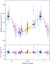 |
Fig. 3. Upper panel: radial velocity measurements for HD 50169, plotted against orbital phase. The solid curve corresponds to the orbital solution given in Sect. 5. The time T0 of periastron passage is adopted as phase origin. Bottom panel: plot of the differences O − C between the observed values of the radial velocity and the predicted values computed from the orbital solution. The dotted lines correspond to ±1 rms deviation of the observational data about the orbital solution (dashed line). Open triangles (dark violet) represent data from Carrier et al. (2002) and asterisks (turquoise) ESO CASPEC observations from Mathys & Hubrig (1997) and Mathys (2017); all other symbols have the same meaning as in Fig. 2. |
The mass function is exceptionally small. For instance, among the Ap binaries for which the orbital elements are listed by Carrier et al. (2002) or by Mathys (2017), only HD 200405 has a lower mass function, f(M) = 0.00010. However, this most likely results from the low inclination of the orbital plane, based on the (different) arguments given in both studies.
By contrast, if we assume that the axis of rotation of the Ap component of HD 50169 is roughly perpendicular to the orbital plane, the inclination of the latter must be rather high because we found in Sect. 4 that i is of the order of either 40° or 92°. Thus, the low value of f(M) must reflect the low mass of the secondary.
Assuming that the mass of the Ap star is of the order of 2 M⊙, for i = 40°, we derive a 1σ upper limit of ∼0.55 M⊙ for the mass of its companion. For i = 92°, this upper limit is reduced to ∼0.35 M⊙. These upper limits correspond to spectral types K7–M1 or M2–M3 (on the main sequence), respectively. In either case, the secondary of HD 50169 would certainly be one of the latest-type companions known of any Ap star. It might possibly even be a late-M or early-L star, given the uncertainty on the mass function.
6. Discussion
Since the existence of Ap stars with unexpectedly long rotation periods became apparent, and as more were progressively found, some of them with ever longer periods, the question has repeatedly arisen whether there were other differences distinguishing them from their faster-rotating counterparts. This question is relevant not only to decide whether the short- and long-period Ap stars constitute two different classes of objects, or if they belong to a single, mostly uniform group. Answering it is also potentially important to shed light onto the physical mechanisms that must be at play to achieve extremely slow rotation, or more generally, the huge differentiation of rotation rates among Ap stars.
In his extensive study of the magnetic properties of Ap stars with resolved magnetically split lines, Mathys (2017) used a number of numerical parameters to characterise the behaviour of the sample stars and to investigate possible trends among them. HD 50169 is now the longest-period star for which these parameters are fully determined. Their consideration provides the first opportunity to test how different HD 50169 is from less slowly rotating Ap stars, or how similar to them.
The average value of the mean magnetic field modulus of HD 50169 over its rotation period is ⟨B⟩av = 5181 G. This is fully consistent with the trend illustrated in Fig. 2 of Mathys (2017), according to which magnetic fields in excess of 7.5 kG are found only in Ap stars with rotation periods shorter than 150 d. The ratio between the extrema of the mean magnetic field modulus, q = 1.43, unambiguously puts the representative point of HD 50169 in the upper right quadrant of Fig. 4 of Mathys (2017). This strengthens the suspicion that the relative amplitude of the ⟨B⟩ variations tends to be greater in longer period stars. The degree of anharmonicity of the ⟨B⟩ variation curve in HD 50169 is well within the range observed in other stars with periods of several years (see Fig. 5 of Mathys 2017). The ratio of the rms longitudinal field (Bohlender et al. 1993), ⟨Bz⟩rms = 1294 G, to ⟨B⟩av is 0.25, also well within the typical range (see Fig. 8 of Mathys 2017). The combination of q = 1.43 with a value r = −0.96 of the ratio of the smaller (in absolute value) to the larger (in absolute value) extremum of ⟨Bz⟩ is consistent with the idea that large relative amplitudes of variation of the field modulus are observed in stars for which both poles come alternately into sight (see Fig. 9 of Mathys 2017). The phase difference (0.579) between the fundamentals of the fits of the measurements of ⟨Bz⟩ and ⟨B⟩ by functions of the forms given in Eqs. (5) and (6) is well within one of the “normality bands” of Fig. 11 of Mathys (2017).
In summary, in all respects, HD 50169 is a “well-behaved” Ap star that does not exhibit any of the “anomalies” found in several of the stars studied by Mathys (2017). This is consistent with the view that no fundamental difference distinguishes the longest-period Ap stars from the rest of the class, or in other words, that the Ap stars constitute a single unified class of objects spanning an exceptionally broad range of rotation rates, but otherwise having similar physical properties. However, this does not imply that there is no correlation between the rotation periods and other properties of Ap stars. The apparent dichotomy in the distribution of the magnetic field strengths between stars with periods shorter and longer than 150 days reported by Mathys (2017) is an example of such a correlation, and this author discussed other possible connections between the geometric structure of the magnetic field and the rotation period, for example. These correlations can only be evidenced and confirmed through studies of statistically significant samples of stars, however.
At present, this statistical significance is at least partially achieved over three orders of magnitude, from 100 to a few 102 d. Extending it to higher orders of magnitude represents a daunting challenge. The first stellar magnetic field was discovered ∼2.5 rotation periods of HD 50169 ago; ∼1.7 such period elapsed since the interest of the long-period Ap stars was recognised; and less than one period of this star has been completed since systematic searches for Ap stars with resolved magnetically split lines have started. On these timescales, the difference (∼7 yr) between its period and that of HD 9996, which was previously the longest-period Ap star for which magnetic measurements had been obtained over a full rotation cycle, represents a considerable step. In the broader context of the five orders of magnitude (or more) spanned by the periods of the Ap stars, it is hardly meaningful, however.
The progress that can be achieved towards improved knowledge of the most slowly rotating Ap stars is by nature incremental because the only way to increase the time base over which relevant observations are available is to await the passage of time. Most likely, the star that will someday overturn HD 50169 as the longest-period Ap star with full coverage of the magnetic variation curve will only have a rotation period a few years, or possibly some decades, longer. This does not detract from the scientific value of monitoring the magnetic fields of the extremely slowly rotating Ap stars. On the contrary, we owe it to the next generations to make sure that we continue to collect the relevant data on a sufficiently regular basis, avoiding gaps in the time series that may severely jeopardise future analyses, so that eventually our successors can successfully achieve complete knowledge of those fascinating stars that hardly rotate at all. The legacy of previous generations opens the realistic prospect of achieving in our lifetime full knowledge of a star such as γ Equ (see Bychkov et al. 2016, and references therein). That this star is no longer unique, and that there must exist instead a significant population of Ap stars with periods of the order of centuries, does not exonerate us from the responsibility of documenting the behaviour of these stars. If we failed to fulfil this responsibility for continuity, our carelessness would deserve to be condemned by our descendants.
Acknowledgments
We are grateful to G. W. Preston and S. J. Adelman for their help in retrieving the date and time at which the spectrum from which Preston (1971) estimated the mean magnetic field modulus of HD 50169 was acquired. Parts of this study were carried out during a stay of GM in the Department of Physics & Astronomy of the University of Western Ontario (London, Ontario, Canada) funded by the ESO Science Support Discretionary Fund (SSDF), and a stay of SH at the ESO office in Santiago within the framework of the ESO Santiago visitors programme. Thanks are due to ESO for its financial support of these science stays, and to the respective host institutions for their welcome. IIR (RSF grant No. 18-12-00423), and DOK, EAS and IAY (RSF grant No. 14-50-00043) gratefully acknowledge the Russian Science Foundation for partial financial support. This research has made use of the SIMBAD database, operated at the CDS, Strasbourg, France.
References
- Adelman, S. J. 1973, ApJS, 26, 1 [NASA ADS] [CrossRef] [Google Scholar]
- Babcock, H. W. 1947, ApJ, 105, 105 [NASA ADS] [CrossRef] [Google Scholar]
- Babcock, H. W. 1948, ApJ, 108, 191 [NASA ADS] [CrossRef] [Google Scholar]
- Babcock, H. W. 1951, ApJ, 114, 1 [NASA ADS] [CrossRef] [Google Scholar]
- Babcock, H. W. 1958, ApJS, 3, 141 [NASA ADS] [CrossRef] [Google Scholar]
- Belopolsky, A. 1913, Astron. Nachr., 195, 159 [NASA ADS] [CrossRef] [Google Scholar]
- Bohlender, D. A., Landstreet, J. D., & Thompson, I. B. 1993, A&A, 269, 355 [NASA ADS] [CrossRef] [Google Scholar]
- Bychkov, V. D., Bychkova, L. V., & Madej, J. 2016, MNRAS, 455, 2567 [NASA ADS] [CrossRef] [Google Scholar]
- Carrier, F., North, P., Udry, S., & Babel, J. 2002, A&A, 394, 151 [NASA ADS] [CrossRef] [EDP Sciences] [Google Scholar]
- Dall, T. H. 2005, CES Users Manual, Issue 1.3, ESO [Google Scholar]
- Deutsch, A. J. 1956, PASP, 68, 92 [NASA ADS] [CrossRef] [Google Scholar]
- Hensberge, H., Manfroid, J., Renson, P., et al. 1984, A&A, 132, 291 [NASA ADS] [Google Scholar]
- Hubrig, S., Järvinen, S. P., Madej, J., et al. 2018, MNRAS, 477, 3791 [NASA ADS] [Google Scholar]
- Kochukhov, O., Bagnulo, S., Wade, G. A., et al. 2004, A&A, 414, 613 [NASA ADS] [CrossRef] [EDP Sciences] [Google Scholar]
- Landstreet, J. D. 1988, ApJ, 326, 967 [NASA ADS] [CrossRef] [Google Scholar]
- Landstreet, J. D., & Mathys, G. 2000, A&A, 359, 213 [NASA ADS] [Google Scholar]
- Mathys, G. 1990, A&A, 232, 151 [NASA ADS] [Google Scholar]
- Mathys, G. 1991, A&AS, 89, 121 [NASA ADS] [Google Scholar]
- Mathys, G. 2017, A&A, 601, A14 [NASA ADS] [CrossRef] [EDP Sciences] [Google Scholar]
- Mathys, G., & Hubrig, S. 1997, A&AS, 124, 475 [NASA ADS] [CrossRef] [EDP Sciences] [Google Scholar]
- Mathys, G., & Lanz, T. 1992, A&A, 256, 169 [NASA ADS] [Google Scholar]
- Mathys, G., Hubrig, S., Landstreet, J. D., Lanz, T., & Manfroid, J. 1997, A&AS, 123, 353 [NASA ADS] [CrossRef] [EDP Sciences] [Google Scholar]
- Mathys, G., Romanyuk, I. I., Kudryavtsev, D. O., et al. 2016, A&A, 586, A85 [NASA ADS] [CrossRef] [EDP Sciences] [Google Scholar]
- Metlova, N. V., Bychkov, V. D., Bychkova, L. V., & Madej, J. 2014, Astrophys. Bull., 69, 315 [NASA ADS] [CrossRef] [Google Scholar]
- Preston, G. W. 1970a, PASP, 82, 878 [NASA ADS] [CrossRef] [Google Scholar]
- Preston, G. W. 1970b, in IAU Colloq. 4: Stellar Rotation, ed. A. Slettebak, 254 [Google Scholar]
- Preston, G. W. 1971, ApJ, 164, 309 [NASA ADS] [CrossRef] [Google Scholar]
- Renson, P., & Manfroid, J. 2009, A&A, 498, 961 [NASA ADS] [CrossRef] [EDP Sciences] [Google Scholar]
- Rice, J. B. 1988, A&A, 199, 299 [NASA ADS] [Google Scholar]
- Romanyuk, I. I., Semenko, E. A., & Kudryavtsev, D. O. 2014, Astrophys. Bull., 69, 427 [NASA ADS] [CrossRef] [Google Scholar]
- Spruit, H. C. 2018, A&A, submitted [arXiv:1810.06106] [Google Scholar]
- Stibbs, D. W. N. 1950, MNRAS, 110, 395 [NASA ADS] [CrossRef] [Google Scholar]
- Sugar, J., & Corliss, C. 1985, Atomic Energy Levels of the Iron-period Elements: Potassium Through Nickel (Washington: American Chemical Society) [Google Scholar]
- Wade, G. A., Mathys, G., & North, P. 1999, A&A, 347, 164 [NASA ADS] [Google Scholar]
- Wolff, S. C. 1975, ApJ, 202, 127 [NASA ADS] [CrossRef] [Google Scholar]
Appendix A: Tables
Mean magnetic field modulus and radial velocity measurements.
Mean longitudinal magnetic field measurements.
All Tables
All Figures
|
Fig. 1. Upper panel: mean longitudinal magnetic field of HD 50169 against rotation phase. The different symbols identify the source and/or instrumental configuration from which the ⟨Bz⟩ value was obtained, as follows: crosses (red): Babcock (1958); filled triangle (violet): Mathys & Hubrig (1997); filled circles (dark blue): Mathys (2017); filled squares (salmon): Romanyuk et al. (2014), and new measurements of spectra obtained with the Main Stellar Spectrograph of the 6 m telescope BTA of the Special Astrophysical Observatory. The long-dashed line (blue) is the best fit of the observations by a cosine wave and its first harmonic, see Eq. (5). The short-dashed line (green) corresponds to the superposition of low-order multipoles discussed in Sect. 4. Lower panel: differences O − C between the individual ⟨Bz⟩ measurements and the best-fit curve against rotation phase. The dotted lines (blue) correspond to ±1 rms deviation of the observational data about the fit (red dashed line). The symbols are the same as in the upper panel. |
| In the text | |
|
Fig. 2. Upper panel: mean magnetic field modulus of HD 50169 against rotation phase. The different symbols identify the source and/or instrumental configuration from which the ⟨B⟩ value was obtained, as follows: filled circles (dark blue): CAT + CES LC; open circles (steel blue): CAT + CES SC; filled hexagon (sea green): 3.6 m + CES LC; filled triangle (violet): CFHT + Gecko (all previous from Mathys et al. 1997; Mathys 2017); five-pointed open stars (orange): 3.6 m + CES VLC; four-pointed open stars (light green): UT2 + UVES; filled pentagons (yellow): 3.6 m + HARPS; filled square (salmon): Preston (1971). The long-dashed line (blue) is the best fit of the observations by a cosine wave and its first harmonic, see Eq. (6). The short-dashed line (green) corresponds to the superposition of low-order multipoles discussed in Sect. 4. Lower panel: differences O − C between the individual ⟨B⟩ measurements and the best-fit curve, against rotation phase. The dotted lines (blue) correspond to ±1 rms deviation of the observational data about the fit (red dashed line). The symbols are the same as in the upper panel. |
| In the text | |
|
Fig. 3. Upper panel: radial velocity measurements for HD 50169, plotted against orbital phase. The solid curve corresponds to the orbital solution given in Sect. 5. The time T0 of periastron passage is adopted as phase origin. Bottom panel: plot of the differences O − C between the observed values of the radial velocity and the predicted values computed from the orbital solution. The dotted lines correspond to ±1 rms deviation of the observational data about the orbital solution (dashed line). Open triangles (dark violet) represent data from Carrier et al. (2002) and asterisks (turquoise) ESO CASPEC observations from Mathys & Hubrig (1997) and Mathys (2017); all other symbols have the same meaning as in Fig. 2. |
| In the text | |
Current usage metrics show cumulative count of Article Views (full-text article views including HTML views, PDF and ePub downloads, according to the available data) and Abstracts Views on Vision4Press platform.
Data correspond to usage on the plateform after 2015. The current usage metrics is available 48-96 hours after online publication and is updated daily on week days.
Initial download of the metrics may take a while.