| Issue |
A&A
Volume 623, March 2019
|
|
|---|---|---|
| Article Number | A51 | |
| Number of page(s) | 10 | |
| Section | The Sun | |
| DOI | https://doi.org/10.1051/0004-6361/201834216 | |
| Published online | 04 March 2019 | |
Spatial power spectrum of the photospheric magnetic field during solar minimum
1
Center for Space Physics, Boston University, 725 Commonwealth Avenue, Boston, MA 02215, USA
e-mail: This email address is being protected from spambots. You need JavaScript enabled to view it.
2
ReSoLVE Centre of Excellence, Space Climate Research Unit, University of Oulu, PO Box 3000, 90014 Oulu, Finland
e-mail: This email address is being protected from spambots. You need JavaScript enabled to view it.
, This email address is being protected from spambots. You need JavaScript enabled to view it.
Received:
10
September
2018
Accepted:
28
January
2019
Abstract
Context. During solar minima the spatial power spectrum of the photospheric magnetic field is dominated by the low-degree zonal (axisymmetric; m = 0) harmonic components, reflecting the large polar coronal holes of unipolar magnetic field. However, measuring polar fields is difficult because of the unequal visibility of the two poles during most of the year and the small line-of-sight component of the roughly radial field at high solar latitudes.
Aims. In this paper we derive the spatial power spectrum of the photospheric magnetic field in terms of the harmonic coefficients of the radial component (Br) as well as in terms of the harmonic coefficients of the internal potential (known as Gauss coefficients). We calculate the zonal spatial power spectrum using Mount Wilson Observatory synoptic maps from 1995–1996, during the solar minimum between solar cycles 22 and 23, and investigate how filling or not filling the polar data gaps affects the zonal harmonic coefficients.
Methods. We eliminated the vantage point effect by removing the highest 5° of the measured magnetic field and calculating the latitudinal profile of the zonal median field over the two years, which ensured equal latitudinal data coverage of both solar hemispheres. We then derived the zonal harmonic coefficients using this latitudinal profile of Br.
Results. We find that when the polar data gaps are left unfilled, a strong artificial power above l = 8 is produced. Only the first five zonal harmonic coefficients can be considered reliable in this case. Therefore polar filling is essential to obtain a realistic spatial power spectrum. Filling the polar gap with a constant (non-zero) value yields zonal harmonics that are reliable up to l = 9. We find that the zonal octupole component contributes most to the total spatial power, more than the zonal dipole, even during the solar minimum conditions. This difference is seen more clearly in the case of polar filling. We also prove that the asymmetry of the polar fields during this solar minimum is statistically significant.
Conclusions. Our results emphasize the importance of filling the polar data gaps in order to obtain a correct estimate of the spatial power spectrum of the photospheric field. This helps in estimating the reliability of polar fields and the large-scale structure in synoptic maps of different origin. Our results also verify the asymmetric nature of the polar fields, which is important for the heliospheric magnetic field and for solar dynamo modeling.
Key words: Sun: photosphere / Sun: magnetic fields / Sun: corona / Sun: activity
© ESO 2019
1. Introduction
The large-scale photospheric magnetic field is very closely axisymmetric during solar minima with extended unipolar regions (polar coronal holes) around the heliographic poles. This is demonstrated in Fig. 1 by a Mount Wilson Observatory (MWO) synoptic map of the radial magnetic field (Br) for Carrington rotation (CR) 1910 (June 1996) during the solar minimum between cycles 22 and 23. Except for a large bipolar active region (AR) around the equator and a few smaller ARs (some including sunspots), the background field is dominated by a region of mixed polarity from −60° to 60° latitude and the large polar coronal holes of uniform polarity. (We note that the color scale is adjusted to the polar magnetic field, not to the strong magnetic field of sunspots that can be several orders of magnitude higher.) This map was calculated from the original line-of-sight measurements of the photospheric magnetic field (Blos) under the assumption that the magnetic field is radial on the solar surface so that Br = Blos/sinθ, where θ is the colatitude. The radial field assumption was first suggested by Svalgaard et al. (1978), based on Wilcox Solar Observatory (WSO) magnetograms using the Fe I line (525.02 nm). Evidence that the photospheric magnetic field is approximately radial was also found by Petrie & Patrikeeva (2009) and Gosain & Pevtsov (2013). It is necessary to use this (or some other) assumption about the orientation of the field because photospheric vector magnetic field observations started only in the 2000s.
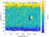 |
Fig. 1. Synoptic map of the MWO photospheric radial magnetic field for CR 1910. |
The photospheric field is most commonly assumed to be radial when using the potential field source surface (PFSS) model to calculate the potential (current-free) magnetic field in the corona. The PFSS model also assumes the coronal field to become radial at the source surface distance Rss, which is typically assumed to be at 2.5 solar radii (Wang & Sheeley 1992).
Since the line-of-sight component of a radial field approaches zero toward the heliographic poles, measurements at high latitudes become increasingly noisy and uncertain. Therefore, the MWO synoptic maps, which are interpolated to a uniform heliographic longitude-latitude grid of 971 × 512, contain missing values at the highest latitudes (see the white unfilled polar areas in Fig. 1).
Since the ecliptic plane is tilted by 7.25° with respect to the solar equator, the polar regions of the Sun are not equally visible during most of the year. This is often referred to as the vantage point or b0 angle problem, resulting in unequal polar data gaps when the Earth is at northern or southern heliographic latitudes. The radial magnetic field in Fig. 1 includes some dubious strong opposite-polarity values at the northern and southern edges of the measured synoptic map (dark blue spots at the northern edge and yellow spots at the southern edge), which are not expected in a unipolar coronal hole. These strong opposite-polarity values do not appear in the same locations in the next or previous CR where the respective heliographic latitudes are better visible. This indicates that these are erroneous values that arise from the above mentioned observational difficulties close to the edge of the visible solar disk.
In this paper, two different methods are used to treat the high-latitude data gaps in the photospheric magnetic field. The polar filling method uses a constant non-zero (positive or negative) value to fill in the polar data gap and is called the “constant filling” method. The second method uses zeros in the polar gaps and is hence called the “zero filling” method (also referred to as no polar filling). The paper is organized as follows. The zonal harmonic coefficients are calculated from the latitudinal profile of the radial magnetic field as described in Sect. 2. A method to eliminate the vantage point effect is presented in Sect. 3. Section 4 discusses the effect of polar filling on the zonal harmonics of the photospheric magnetic field, while error estimates of the zonal harmonic coefficients are given in Sect. 5. The zonal spatial power spectrum of the photospheric magnetic field during solar minimum (1995–1996) is presented in Sect. 6. We discuss the results in Sect. 7 and give our conclusions in Sect. 8.
2. Data and methods
2.1. Photospheric magnetic field data
In this study we use MWO photospheric synoptic maps of line-of-sight magnetic field observations for CR 1892–1917, covering the solar minimum years of 1995–1996. MWO data are given in a relatively high-resolution longitude-latitude grid of 971 × 512, which provides a uniform latitudinal resolution of 0.35° at all latitudes. The photospheric data from other stations are given in a longitude – sine-latitude grid, which makes the cell size constant but leads to a decreasing latitudinal resolution toward the poles. As we show here, sufficient resolution at high latitudes is essential for determining the higher-degree zonal harmonic coefficients of the photospheric magnetic field. Moreover, although the Kitt Peak (KP) magnetograms have much higher resolution (1.1 arcsec) at this time than the MWO magnetograms (12.5 or 20 arcsec), we use MWO data because the KP data are known to suffer from errors (Harvey & Munoz-Jaramillo 2015).
Observations of large-scale photospheric magnetic fields (full-disk magnetograms) started on Mount Wilson in the late 1950s and continued until January 2013. Digital calibrated data are available for 1974–2013 (see, e.g., Howard et al. (1983), Ulrich et al. (2002), and references therein). MWO observations started using a Babcock-type magnetograph, and there were several instrument updates, the most significant in 1982, 1994, and 1996. These updates allowed using other spectral lines as well and observing spectral lines with better spectral resolution. They typically observed several fastgrams (aperture size 20 arcsec) and at least one slowgram (aperture size 12.5 arcsec) per day. Synoptic maps are constructed from full-disk observations using all the available data.
Polar data gaps are not filled in the MWO data, which allows us to study the effect of different polar filling methods on the zonal harmonic coefficients. However, it should be noted that the MWO synoptic maps are interpolated to the given longitude-latitude grid from the original observations, which may not have the same resolution and accuracy at all locations. Therefore, we need to empirically determine the highest northern/southern latitude where the measurements are still reliable.
2.2. Definition of harmonic coefficients
The harmonic coefficients  and
and  are defined differently in solar physics and in geomagnetism, which might be confusing for experts of either field. In this section, we aim to clarify these two different definitions.
The coronal magnetic field is commonly estimated with the PFSS model (Wang & Sheeley 1992) with a source surface at a radius of Rss, where the coronal magnetic field becomes radial. The magnetic potential arises both from internal sources inside the inner boundary of the photospheric radius R0 and external sources outside the source surface. The solution of the PFSS model for the radial magnetic field Br gives
![Mathematical equation: $$ \begin{aligned} B_{\rm r} (r,\theta ,\phi )&=-\frac{\partial \Psi }{\partial r}\nonumber \\&=\sum _{l=0}^{\infty }\sum \limits _{m=0}^{l}P_l^m (\cos \theta )(\mathrm{g}_l^m\cos m\phi +h_l^m\sin m\phi )\left(\frac{R_0}{r}\right)^{l+2}\nonumber \\&\quad \times \left[l+1+l\left(\frac{r}{R_{\mathrm{ss} }}\right)^{2l+1}\right] \left[l+1+l\left(\frac{R_0}{R_{\mathrm{ss} }}\right)^{2l+1}\right]^{-1}, \end{aligned} $$](/articles/aa/full_html/2019/03/aa34216-18/aa34216-18-eq3.gif) (1)
(1)
where Ψ is the sum of the internal and external potentials, θ is the colatitude, ϕ is the longitude,  is the Schmidt semi-normalized associated Legendre function, and l and m are the degree and azimuthal order of the spherical harmonics, respectively. In the photosphere (r = R0), Br reduces to
 (2)
(2)
In solar physics,  and
and  are therefore the harmonic coefficients of the spherical harmonics expansion of the radial magnetic field component in the photosphere. These harmonic coefficients are related to
  and
and  , the harmonic coefficients of the internal potential ΨI,
 (3)
(3)
through the following equations:
![Mathematical equation: $$ \begin{aligned} \mathrm{g}_l^m=(l+1){\mathrm{g}\prime }_l^m\left[1+\frac{l}{l+1}\left(\frac{R_0}{R_{\mathrm{ss} }}\right)^{2l+1}\right], \end{aligned} $$](/articles/aa/full_html/2019/03/aa34216-18/aa34216-18-eq11.gif) (4)
(4)
![Mathematical equation: $$ \begin{aligned} h_l^m=(l+1){h\prime }_l^m\left[1+\frac{l}{l+1}\left(\frac{R_0}{R_{\mathrm{ss} }}\right)^{2l+1}\right]. \end{aligned} $$](/articles/aa/full_html/2019/03/aa34216-18/aa34216-18-eq12.gif) (5)
(5)
We note that in these harmonic coefficients, the terms (l + 1) and (l + 1)
 come from internal sources, while the term proportional to l/(l + 1)(R0/Rss)2l + 1 is of external origin. In geomagnetism, however, the notations
  and
and  are generally used for the harmonic coefficients of the internal potential (Eq. (3)), also known as Gauss coefficients. To be consistent with earlier literature on solar and heliospheric physics, we continue to use
  and
and  for the harmonic coefficients of Br and
  and
and  for the Gauss coefficients of ΨI.
The radial magnetic field in the photosphere arising from internal sources alone can be obtained from ΨI as follows:
 (6)
(6)
It can be readily seen in Eqs. (4) and (5) that  and
and  approach (l + 1)
 and (l + 1)
 , respectively, as l approaches infinity, which means that the external sources become negligible in the photospheric magnetic field for high values of l. Only the lowest-degree harmonics of the photospheric field are slightly affected by external sources. For Rss = 2.5R0, the relative contribution of external sources to the dipole component (l = 1) of the photospheric magnetic field is only 3.2%. Considering the large uncertainty of the measured photospheric magnetic field at high heliographic latitudes, the contribution of external sources to the photospheric magnetic field can be safely neglected. In this case, the photospheric magnetic field comes purely from the internal potential, and the observed radial magnetic field is given by Eq. (6) (or Eq. (2) with coefficients including only the internal contribution).
Multiplying both sides of Eq. (6) by the spherical harmonics  (cos θ) cosmϕ and
  (cos θ) sinmϕ and integrating over the solar surface, we obtain the solution for the unknown Gauss coefficients
  and
and  , respectively (Backus et al. 1996):
 (7)
(7)
Here we made use of the following orthogonality relationships of the Schmidt semi-normalized spherical harmonics:
 (8)
(8)
and
 (9)
(9)
where δij is the Kronecker delta.
For photospheric magnetic field data with a longitude–latitude grid of Nϕ × Nθ, the solid angle of a grid cell ΔΩ = sinθΔθΔϕ decreases with latitude, where Δθ = π/Nθ and Δϕ = 2π/Nϕ. The discrete representation of Eq. (7) then yields the Gauss coefficients as follows:
 (10)
(10)
The zonal (m = 0) Gauss coefficients  can then be expressed as
 (11)
(11)
where  is the zonal mean line-of-sight magnetic field at the colatitude of θi.
In order to exclude outliers (e.g., newly emerged sunspots with a magnetic field orders of magnitude higher than the background photospheric field), we use the zonal median instead of the zonal mean in Eq. (11) to calculate the first 24 zonal Gauss coefficients of the internal potential. The latitudinal profiles can be reconstructed from the first 24 zonal harmonics as follows (cf. Eqs. (2) and (6)):
 (12)
(12)
The reconstruction based on the first 24 harmonics is quite sufficient when studying the large-scale structure of the photospheric field.
2.3. Definition of spatial power spectrum
The main challenge in defining the spatial power spectrum of the photospheric magnetic field is to find the correct normalization for the harmonic coefficients. Any real function f(θ, ϕ) can be expanded in terms of Schmidt semi-normalized spherical harmonics as
 (13)
(13)
in analogy with Eq. (2). As already noted above, the spherical harmonics form a complete orthogonal system under integration over the unit sphere (cf. Eqs. (8) and (9)). It is in fact a generalized Fourier series that transforms a bivariate function f(θ, ϕ) from the two-dimensional domain [θ, ϕ] (unit sphere) into the two-dimensional domain of [l, m]. In this section, we derive the generalized Parseval theorem for the Schmidt semi-normalized spherical harmonics expansion and define the corresponding spatial power spectrum.
The total power of f(θ, ϕ) is defined as the integral of the function squared, divided by the area of its domain:
![Mathematical equation: $$ \begin{aligned} \frac{1}{4\pi }\int f^2\mathrm{d} \Omega&=\frac{1}{4\pi }\int \limits _0^{2\pi }\mathrm{d} \phi \int \limits _0^{\pi }\sin \theta \mathrm{d} \theta \nonumber \\&\left[\sum \limits _{l=0}^{\infty }\sum \limits _{m=0}^lP_l^m (\cos \theta )(\mathrm{g}_l^m\cos m\phi +h_l^m\sin m\phi )\right]^2\nonumber \\&= \frac{1}{4\pi }\sum \limits _{l=0}^{\infty }\sum \limits _{m=0}^l\sum \limits _{l\prime =0}^{\infty }\sum \limits _{m\prime =0}^{l\prime }\frac{4\pi }{2l+1}(\mathrm{g}_l^mg_{l\prime }^{m\prime }\delta _{ll\prime }\delta _{mm\prime }+h_l^mh_{l\prime }^{m\prime }\delta _{ll\prime }\delta _{mm\prime })\nonumber \\&=\sum \limits _{l=0}^{\infty }\sum \limits _{m=0}^l\frac{1}{2l+1}\left[(\mathrm{g}_l^m)^2+(h_l^m)^2\right], \end{aligned} $$](/articles/aa/full_html/2019/03/aa34216-18/aa34216-18-eq39.gif) (14)
(14)
where we used the normalization and orthogonality relationships of Eqs. (8) and (9).
Equation (14) gives the total power of f(θ, ϕ) in terms of the squares of its harmonic coefficients. This is the generalized Parseval theorem for the Schmidt semi-normalized spherical harmonics expansion. The scaling factor 1/(2l + 1) comes from the normalization of the Schmidt semi-normalized spherical harmonics (Eq. (8)). We note that for a different (e.g., orthonormal) normalization, this scaling factor would be one.
The total power can also be written as
 (15)
(15)
where
![Mathematical equation: $$ \begin{aligned} S_l^{\mathrm{degree} }=\frac{1}{2l+1}\sum \limits _{m=0}^l\left[(\mathrm{g}_l^m)^2+(h_l^m)^2\right] \end{aligned} $$](/articles/aa/full_html/2019/03/aa34216-18/aa34216-18-eq41.gif) (16)
(16)
is the power per degree.  is often referred to as the power spectrum of function f in the literature. However, the power spectrum of white noise would rise infinitely if this normalization were used (Hipkin 2001). Therefore, it is more appropriate to define the power spectrum as the power per independent mode:
![Mathematical equation: $$ \begin{aligned} S_l^{\mathrm{mode} }=\frac{1}{2l+1}S_l^{\mathrm{degree} }= \frac{1}{(2l+1)^2}\sum _{m=0}^l\left[(\mathrm{g}_l^m)^2+(h_l^m)^2\right]. \end{aligned} $$](/articles/aa/full_html/2019/03/aa34216-18/aa34216-18-eq43.gif) (17)
(17)
Here the additional 1/(2l + 1) factor comes from the averaging over the independent modes for each degree l. This definition produces a constant power spectrum for white noise.
The total power of the magnetic field can be calculated from the internal potential as follows:
 (18)
(18)
where the surface gradient ∇s is defined as
 (19)
(19)
Inserting the spherical harmonics expansion of the internal potential (Eq. (3)) into Eq. (18), we can express the total power of the magnetic field in terms of the Gauss coefficients  and
and  (see detailed derivation in Backus et al. (1996)):
![Mathematical equation: $$ \begin{aligned} \frac{1}{4\pi }\int \mathbf B ^2\mathrm{d} \Omega =\sum \limits _{l=1}^{\infty }(l+1)\left(\frac{R_0}{r}\right)^{2l+4}\sum \limits _{m=0}^l\left[({\mathrm{g}\prime }_l^m)^2+({h\prime }_l^m)^2\right]. \end{aligned} $$](/articles/aa/full_html/2019/03/aa34216-18/aa34216-18-eq48.gif) (20)
(20)
In the photosphere (r = R0), the power-per-degree spectrum is
![Mathematical equation: $$ \begin{aligned} S_l^{\mathrm{degree} }=(l+1)\sum \limits _{m=0}^l\left[({\mathrm{g}\prime }_l^m)^2+({h\prime }_l^m)^2\right] \end{aligned} $$](/articles/aa/full_html/2019/03/aa34216-18/aa34216-18-eq49.gif) (21)
(21)
and the power-per-independent-mode spectrum is
![Mathematical equation: $$ \begin{aligned} S_l^{\mathrm{mode} }&=\frac{1}{2l+1}S_l^{\mathrm{degree} }=\frac{l+1}{2l+1}\sum \limits _{m=0}^l\left[({\mathrm{g}\prime }_l^m)^2+({h\prime }_l^m)^2\right] \nonumber \\&=\frac{1}{(l+1)(2l+1)}\sum \limits _{m=0}^l\left[(\mathrm{g}_l^m)^2+(h_l^m)^2\right]. \end{aligned} $$](/articles/aa/full_html/2019/03/aa34216-18/aa34216-18-eq50.gif) (22)
(22)
We here use the latter definition for the spatial power spectrum of the photospheric magnetic field, which is identical to the definition of the geomagnetic spatial power spectrum given by Maus (2008).  provides the average power per independent mode and does not depend on the choice of the coordinate system. The averaging over the independent modes ensures that an uncorrelated noise, the autocorrelation function of which is a Dirac delta, produces the expected constant flat spectrum.
We define the spatial power spectrum of the zonal (m = 0), sectorial (l = m), and tesseral (l ≠ m) harmonic components similarly as the power per independent mode for each degree. The zonal harmonics have only a single mode per degree, the sectorial harmonics have two independent modes per degree, while the tesseral harmonics have 2l − 2. The zonal, sectorial, and tesseral spatial power spectra therefore are the following:
 (23)
(23)
 (24)
(24)
 (25)
(25)
All the spatial power spectra of Eqs. (22)–(25) yield the same constant spectrum for uncorrelated white noise. The zonal spatial power spectrum Eq. (23) gives the relative contributions of the different zonal multipoles (dipole, quadrupole, octupole, hexadecapole, 32-pole, etc.) to the total power of the photospheric magnetic field.
3. Eliminating the vantage point effect
We are interested in the zonal harmonics of the magnetic field that are axisymmetric with respect to the solar rotation axis, therefore we calculated the latitudinal profile of the photospheric magnetic field by taking the zonal median of each Carrington synoptic map for those heliographic latitudes that have no data gaps. The zonal median excludes outstandingly high values of sunspots or active regions and represents the expected value of the large-scale photospheric magnetic field. As an example, we plot the latitudinal profile of the radial magnetic field for three consecutive CRs, CR 1910 (June 1996) through CR 1912 (August 1996) in Fig. 2. As a result of the vantage point effect, the magnetic field profiles cover different latitude ranges with increasing (decreasing) coverage of northern (southern) latitudes as the Earth moves from low heliographic latitudes (June) toward higher northern latitudes.
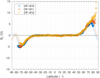 |
Fig. 2. Latitudinal profiles of the radial magnetic field for CR 1910 to 1912. Solid lines with corresponding colors represent the field reconstructed from the first 24 harmonics. |
The three profiles in Fig. 2 nicely agree with each other over most of the overlapping latitude range, except for observations at the highest 5° in either hemisphere for any Carrington rotation. In most cases, the radial magnetic field tends to be underestimated at the southern and northern ends of the profiles, which is due to the erroneous opposite-polarity pixels at the edges of the synoptic map, as shown for CR 1910 in Fig. 1. Because the large-scale photospheric magnetic field is not expected to change much during one CR at the time of solar minimum, the three magnetic field profiles should be very similar to each other. The latitudinal profile of the photospheric magnetic field indeed hardly changed from CR 1910 to CR 1911 (see the blue and red symbols in Fig. 2), except that the field magnitude in CR 1911 started to decline at higher latitude in the northern hemisphere and at lower latitude in the southern hemisphere. During the following rotation (CR 1912), when the northern hemisphere was best visible, the magnetic field monotonically increased toward the pole (yellow symbols in Fig. 2), and no decline was observed in the northern hemisphere. At the same time, a decline was observed in the southern hemisphere at lower latitudes than in the two previous rotations. This further confirms that the observed decline of the magnetic field at the highest latitudes (in both hemispheres) during solar minimum times is an artifact of the vantage point effect and should be removed or corrected for.
We have calculated the first 24 zonal Gauss coefficients as well as the first 24 zonal harmonic coefficients of Br for the latitudinal profiles of Fig. 2 using the method described in Sect. 2.2. The harmonic coefficients shown in Fig. 3 do not reflect the relative strength of the different zonal multipoles. The zonal octupole (l = 3) is the largest harmonic coefficient of Br, while the zonal dipole (l = 1) is the largest Gauss coefficient of the internal potential. However, the zonal spatial power of the photospheric magnetic field during solar minimum is roughly equally divided between these two harmonics, as we show in detail in Fig. 10.
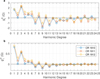 |
Fig. 3. Panel a: zonal harmonic coefficients of the radial magnetic field Br. Panel b: zonal Gauss coefficients of the internal potential ΨI for CR 1910–1912, calculated without polar filling (zero filling). |
The harmonic coefficients for CR 1910 through CR 1912 are quite different, as shown in Fig. 3, because the profiles are different at high latitudes. This is partly due to the different latitudinal data coverage and partly due to the (erroneous) decline of the polar magnetic field at different latitudes.
We have also reconstructed the radial magnetic field for the three rotations using the 24 Gauss coefficients in Fig. 3 (see Eq. (12)) and included the reconstructions as lines in Fig. 2. The reconstructed field tries to reproduce the missing (zero) values of the high-latitude data gaps.
Fig. 3 shows that the low-degree odd zonal harmonics, the dipole (l = 1), octupole (l = 3), and 32-pole (l = 5), are all positive. They are mainly responsible for producing the opposite-polarity (but equally strong) field in the northern and southern high-latitude regions. Interestingly, the higher-degree odd zonal harmonics (l = 7, 9, 11, and 13) in Fig. 3 all have opposite (negative) sign to the low-degree odd harmonics. These higher-degree odd harmonics tend to decrease the polar field, aiming to reproduce the zero magnetic field in the polar data gaps.
The even zonal harmonics reduce the dominant polar field in one hemisphere and increase it in the other, producing an asymmetry in the strength of the observed polar magnetic fields. The vantage point effect introduces an artificial asymmetry between the simultaneous values of the two polar fields because of the different visibility of the highest northern and southern latitudes. The vantage point effect is also clearly recognizable in Fig. 3. When both polar regions are approximately equally visible, as in CR 1910 (June 1996), the even zonal harmonic coefficients are very small (see Fig. 3). However, when the southern polar region is less visible, as in CR 1911 (July 1996), the observed magnetic field covers a larger latitude range in the north, and a stronger field is measured there than in the south. This results in larger even zonal harmonic coefficients for CR 1911. When the southern polar region is even less visible in CR 1912 (August 1996), the even harmonic coefficients become still larger. Thus, the vantage point effect produces artificial variability in the harmonic structure of the photospheric magnetic field, which is manifested in the even zonal harmonics.
In order to eliminate the vantage point effect and the above-discussed erroneous values at the highest observed latitudes, we used the following procedure. We took two years (1995–1996) of synoptic maps of the photospheric magnetic field. From each synoptic map we removed observations at the highest measured 5° of northern and southern latitudes. Then we calculated the zonal medians of the radial magnetic field for each synoptic map to obtain a latitudinal profile for each CR (as in Fig. 2). Finally, we calculated the medians at each latitude bin over the two years (1995–1996) to obtain the median latitudinal profile of the radial magnetic field for this solar minimum. This profile is plotted in blue in Fig. 4. By using two full years of observations, we achieved sufficient statistics in the latitude range of ±80° and ensured an equal data coverage of the northern and southern hemispheres.
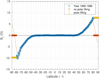 |
Fig. 4. Median latitudinal profile of the radial magnetic field over 1995–1996 with constant (yellow) and zero (red) polar filling. Solid lines with corresponding colors represent the field reconstructed from the first 24 harmonics. |
The observed radial magnetic field profile in Fig. 4 increases nearly monotonically toward the poles. Despite some variations at high latitudes (especially in the south), it does not show the systematic decline at the highest measured latitudes, as seen for individual CRs in Fig. 2 even at lower latitudes. Accordingly, this artifact has been successfully eliminated by removing the erroneous observations at the highest measured 5° of latitude in each synoptic map. As seen in Fig. 4, the median strength of the radial magnetic field at the highest southern latitude of −80° (about 10 G) was moreover greater than that at the highest northern latitude of 80° (about 7.5 G) during this solar minimum. We note that this hemispheric asymmetry in the mid-1990s is consistent with a statistically significant polar field imbalance at this time (Zhao et al. 2005; Virtanen & Mursula 2010, 2016; Erdős & Balogh 2010; Petrie 2015) and follows the general pattern of the southward-shifted heliospheric current sheet in the declining to minimum phase of each solar cycle (Mursula & Hiltula 2003).
4. Effect of polar filling on zonal harmonic coefficients
We now investigate how polar filling affects the zonal harmonics of the radial magnetic field. In Fig. 4 the missing high-latitude field values poleward of ±80° are treated with two different methods. In the first method, we use zeros in the polar gaps (red in Fig. 4), which is referred to as zero filling or no polar filling. In the second method, the polar gaps are filled with the value of the median profile at the highest northern or southern latitude of ±80° (yellow in Fig. 4), which is called constant filling. We acknowledge that this is quite a crude polar filling method, and we used it only as a simple approximation to explore the differences between polar filling and no polar filling. More sophisticated polar filling methods typically apply 1D or 2D spatial interpolation using magnetic field values from lower latitudes and/or temporal interpolation between polar field values observed during the times when the northern or southern pole is visible. For a comprehensive review of different polar field interpolation methods, see Sun et al. (2011).
The first 24 zonal harmonic coefficients of Br and the first 24 zonal Gauss coefficients calculated from the latitudinal profiles of Fig. 4 with and without polar filling are shown in Fig. 5. The lowest three odd harmonics have the same sign for the two cases, but they are clearly larger for constant filling than for zero filling. The difference between the two methods is even more striking for higher odd harmonics (nine and beyond). While these harmonics are practically negligible for polar filling, they have a negative (opposite to the low odd harmonics) sign and a large magnitude for no polar filling.
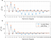 |
Fig. 5. Panel a: zonal harmonic coefficients of Br. Panel b: zonal Gauss coefficients of ΨI for 1995–1996, calculated from the filled (constant filling) and unfilled (zero filling) radial magnetic field profiles in Fig. 4. |
The radial magnetic field profiles reconstructed from the first 24 zonal Gauss coefficients (using Eq. (12)) are plotted in Fig. 4 as lines with colors that match the two cases. For constant filling, the reconstructed profile almost perfectly overlaps the observed field values of the profile as well as the part of polar filling. The reconstructed profile for zero filling, on the other hand, fails to overlap the observed field values already at the latitude of about ±75° because it attempts to reproduce the zero polar values. By trying to reproduce the polar zero field, the reconstructed profile even produces opposite-polarity values at the highest latitudes beyond about ±85°. This is obviously another unphysical artifact that only comes from the mathematical properties of the spherical harmonic functions. The limited spatial resolution of the first 24 harmonics is not sufficient to reproduce the sharp change in the radial magnetic field from the last measured high-latitude value to the polar zero value in case of no polar filling.
To further clarify the difference between constant filling and zero filling in the harmonic structure of the zonal magnetic field, we calculated the difference (ΔBr) between the measured unfilled and filled radial magnetic field profiles of Fig. 4 and plot them in Fig. 6a. Their difference is a step function at the highest observed latitude in both hemispheres. The lowest 24 Gauss coefficients of this double-step function are shown in Fig. 6b. These coefficients are identical with the difference between the two sets of coefficients presented in Fig. 5b. Apparently, adding or subtracting radial magnetic field profiles is equivalent to adding or subtracting their Gauss coefficients because Br is a linear combination of  , as shown in Eq. (12). The profile reconstructed from the first 24 harmonics of the double-step function is also plotted in Fig. 6a. The reconstruction is not perfect and fails to reproduce the polar field by 30–40%. A perfect reconstruction would require an infinite number of harmonic coefficients. We conclude that all odd zonal Gauss coefficients (especially l ≥ 9) are seriously compromised if they are calculated from data with zeros at the poles, that is, from unfilled data. Polar filling is therefore necessary to obtain a realistic estimate of the harmonic structure of the zonal magnetic field.
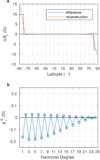 |
Fig. 6. Panel a: difference between the unfilled and filled radial magnetic field profiles of Fig. 4. Panel b: corresponding zonal Gauss coefficients. The field reconstructed from these harmonics is plotted in red in the upper panel. |
In order to illustrate the latitudinal structure of zonal harmonics, we plot the odd (Schmidt semi-normalized) associated Legendre functions  for l = 1−23 in Fig. 7. These functions have the highest absolute values at the poles where the magnetic field cannot be reliably measured. The vertical dashed line marks the highest latitude (80°) of MWO observations used in this study. The latitudinal resolution of 10° of the polar field furthermore cannot resolve harmonics above l = 13 because the corresponding Legendre functions change sign within this one single grid cell (see Fig. 7). Moreover, the weight of the last reliable measurement at 80° in the Legendre functions is much smaller above l = 9 than for lower harmonics. This means that the harmonics above l = 9 do not contribute much to the observed field in the latitude range of ±80°, but they do contribute to the polar filling, especially to the zero filling (see Fig. 5). With the given limitations of high-latitude observations, the zonal harmonic coefficients therefore cannot be reliably determined above the harmonic of l = 9.
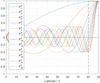 |
Fig. 7. Odd associated Legendre functions |

5. Estimating the error of zonal harmonic coefficients
As shown in Fig. 5, the first four even zonal harmonic coefficients quadrupole (l = 2), hexadecapole (l = 4), 64-pole (l = 6), and 256-pole (l = 8), are negative in the case of polar filling. We now study whether these even zonal harmonics are statistically significant. We can estimate the error of the observed latitudinal profile by calculating the lower and upper quartiles of observations in each latitude bin during the two-year period. The interquartile range contains 50 percent of observations, so that it represents the spread or error of observations even if the field distributions might be non-Gaussian. The latitudinal profile of the median radial magnetic field is plotted in Fig. 8 along with the corresponding lower and upper quartiles. Because the even zonal harmonics are responsible for the north-south asymmetry, they attain their maximum (minimum) values for magnetic field profiles with the largest (smallest) possible asymmetry within the interquartile range. Accordingly, the profile of the lower (upper) quartile would result in the highest (lowest) north-to-south polar field ratio. The harmonic coefficients of the magnetic field profiles for the upper and lower quartiles would therefore yield the extreme values of the even zonal harmonics.
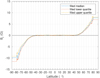 |
Fig. 8. Median, lower quartile, and upper quartile of the radial magnetic field during the solar minimum of 1995–1996. Missing data at high latitudes are filled with the last reliably measured value in each latitudinal profile. |
The odd harmonics would attain their maximum (minimum) values for magnetic field profiles with the highest (lowest) absolute values of polar fields within the interquartile range. This means that the harmonic coefficients of a magnetic field profile that follows the lower quartile in the southern hemisphere and the upper quartile in the northern hemisphere would yield the maximum value of the odd harmonic coefficients. Similarly, the harmonic coefficients of a magnetic profile that follows the upper quartile in the southern hemisphere and the lower quartile in the northern hemisphere would yield the minimum value of the odd harmonic coefficients.
In this way, we obtain the error estimates for the zonal harmonic coefficients of Br and for the Gauss coefficients in the case of polar filling, which are shown in Fig. 9. All harmonic coefficients up to l = 9 are different from zero according to their estimated errors. The high-degree non-zero coefficients (l = 15, 17, 19, 21, 23) in Fig. 9a reflect the assumed constancy of the polar field, and are therefore non-physical. The first four even zonal harmonics represent a statistically significant north-south asymmetry with a stronger magnetic field in the southern polar region. The dominance of the southern polar field is also evident from the magnetic field profile in Fig. 8. The strength of the median radial magnetic field is 9.8+1.7/−0.6 G above 80° southern latitude, while it is 7.8+0.3/−0.9 G in the north. Thus, the interhemispheric polar field difference is about three standard deviations at the confidence level of 98%.
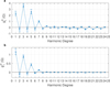 |
Fig. 9. Panel a: zonal harmonic coefficients of Br. Panel b: zonal Gauss coefficients of ΨI with errors estimated from the latitudinal profiles of the radial magnetic field in Fig. 8. |
6. Spatial power spectrum
We calculated the zonal (m = 0) spatial power spectrum of the photospheric magnetic field with and without polar filling using Eq. (23). This represents the spatial power spectrum of the axial magnetic field. The total spatial power spectrum of the photospheric magnetic field can be calculated from Eq. (22) and also includes the sectorial (l = m; Eq. (24)) and tesseral components (l ≠ m; Eq. (25)). This definition of the total spatial power spectrum is the same as the definition of the spatial power spectrum of the geomagnetic field (Maus 2008). Because the large-scale photospheric (and coronal) magnetic field is dominated by the axisymmetric field during solar minimum (see Fig. 7 in Petrie 2013), we restrict our analysis to the zonal spatial power spectrum in this study.
As demonstrated in Fig. 10, the powers of the low odd zonal harmonics (l = 1, 3, and 5) are by far the largest, about two orders of magnitude higher than the power of the low even zonal harmonics (l = 2, 4, 6). For no polar filling, the power of all low zonal harmonics (l < 9) is somewhat smaller than for polar filling, but the power of the high zonal harmonics (l ≥ 9) is larger by 1–3 orders of magnitude. At higher harmonic degrees beyond l = 15 (l = 9), the spectrum flattens for polar filling (no filling), which is an artifact of the constant polar field value (whether zero or not). For a more sophisticated analytical or physics-based polar filling method, such as the commonly used low-degree polynomial surface interpolation or the flux transport modeling method, the spectrum is not expected to flatten beyond l = 15, and the powers of the odd harmonics are expected to be somewhat stronger in the low-degree range (l ≤ 9) because these methods tend to predict stronger fields at the poles than the constant polar filling.
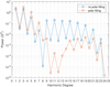 |
Fig. 10. Zonal spatial power spectrum of the photospheric magnetic field during the solar minimum in 1995–1996, calculated from the filled and unfilled radial magnetic field profiles in Fig. 4. |
Interestingly, we find that the zonal octupole component is slightly stronger than the zonal dipole. This difference is seen even more clearly in the (more realistic) case of polar filling. This result is in disagreement with the common view of the solar magnetic field having mainly a dipolar structure during solar minimum times. However, this seemingly surprising result can naturally be understood in terms of the weak dominance of opposite polarity at low latitudes in both hemispheres (see also Figs. 2 and 4). We also note that the octupole component only dominates the photospheric field, not the coronal field, because the higher multipoles decay faster with radial distance.
We can use the maximum power of high harmonics as a credibility threshold or a kind of noise level to determine which harmonic coefficients can be trusted. For no polar filling, this threshold is about 0.2 G2, so that we can trust the corresponding low odd zonal harmonic coefficients only up to l = 5. For constant polar filling, this threshold is almost two orders of magnitude lower, about 4 × 10⁻³ G2, and we can trust both the odd and even zonal harmonic coefficients up to l = 7. This is consistent with the error estimates shown in Fig. 9. A more realistic polar filling method could increase the credibility of the higher-degree zonal harmonics, but the spectrum will be highly model dependent above l = 9 because these harmonics are not constrained by direct observations above ±80° latitude (see Fig. 7).
7. Discussion
The measurement of the photospheric magnetic field is problematic at high heliographic latitudes because the line of sight is nearly perpendicular to the local magnetic field vector. The observed line-of-sight component of the magnetic field becomes smaller and smaller toward the poles, which diminishes the signal-to-noise ratio and increases the error of the inferred radial magnetic field. Bertello et al. (2014) studied uncertainties in synoptic maps and effects on the coronal magnetic field and coronal hole maps derived with the PFSS model. They concluded that uncertainties are largest in active regions during solar maximum. On the other hand, polar fields and the low-degree zonal harmonics are more affected by errors during solar minimum.
The question is what the highest latitudes are in each synoptic map of the photospheric magnetic field where the radial magnetic field calculated from the measured line-of-sight field is still reliable. During solar minima, the high-latitude solar corona has a rather simple structure with little temporal variation. This implies that the large-scale high-latitude photospheric magnetic field is not expected to change much from one CR to the next during the solar minimum conditions.
We have identified the highest latitudes in each MWO synoptic map where the observed zonal median of the magnetic field is still comparable to that obtained from the previous and subsequent CRs. We found that the highest 5° of the measured magnetic field is systematically underestimated, as shown in Fig. 2. Therefore we excluded the observations within the highest 5° of latitude in each synoptic map from further analysis.
Another difficulty of measuring the solar magnetic field especially at high latitudes is the vantage point effect. Owing to the 7.25° tilt of the ecliptic with respect to the heliographic equatorial plane, the polar regions of the Sun are not equally visible from Earth during most of the year. We have shown that the vantage point effect seriously affects the zonal harmonic coefficients calculated for individual synoptic maps of the photospheric magnetic field (Fig. 3). This is true for all harmonics, but especially for the even zonal harmonics that describe the north-south asymmetry of the field. In order to obtain a realistic estimate of the spherical harmonic structure of the axial magnetic field during solar minimum, we have to eliminate the vantage point effect. We have implemented this by calculating the median of the latitudinal profiles of the photospheric field for CRs over two consecutive years to ensure equal and sufficient data coverage of the northern and southern hemispheres.
We have demonstrated that leaving the polar data gaps unfilled results in artificially enhanced high-degree (l ≥ 9) odd zonal harmonic coefficients that have a sign opposite to the dominant dipole polarity (Fig. 5). This comes from the harmonic structure of the artificial step function that is formed at the boundary of the polar data gap (see Fig. 6). Unfilled polar data gaps also significantly diminish the low-degree (l < 9) odd zonal harmonic coefficients. Polar filling is therefore essential before calculating the large-scale harmonic structure of the photospheric magnetic field.
In this study we used a simple polar filling method. We filled the polar gap by a constant magnetic field that is identical with the zonal median field at the highest reliably measured latitude (about 80°) in the respective hemisphere. Although this is not an ideal polar filling method, it proved sufficient to significantly reduce the spurious high zonal harmonic coefficients and helped to calculate a more realistic spatial power spectrum of the photospheric magnetic field during solar minimum conditions (see Figs. 9 and 10). We note that although filling the poles with a constant field value helps to greatly improve the solar magnetic field, it is only an approximate solution to the polar data gap problem. A further refinement could be made, for instance, by extrapolating the latitudinal profiles of the observed magnetic field to the poles.
The main objective of this study is to derive the harmonic structure and spatial power spectrum of the axial photospheric magnetic field during solar minimum conditions, and to provide error estimates for the zonal harmonic coefficients. Our error estimates suggest that only the first nine zonal harmonic coefficients are significantly different from zero in the case of polar filling.
We have also shown that the low even zonal harmonics systematically deviate from zero and have a sign opposite to that of the dominant low odd zonal harmonics. Non-zero even zonal harmonics decrease the polar field in one hemisphere and increase it in the other, leading to a north-south asymmetry. The opposite sign of the even zonal harmonics to the dominant dipole polarity indicates a north-south asymmetry where the southern polar magnetic field is stronger than the northern one.
The asymmetry in the polar fields is clearly recognizable also in the latitudinal profiles of the radial magnetic field (see Figs. 4 and 8). A similar systematic north-south asymmetry has first been reported in the heliospheric magnetic field (Mursula & Hiltula 2003) and later in the photospheric magnetic field observations at WSO (Zhao et al. 2005) and in the coronal field based on six different photospheric databases (Virtanen & Mursula 2016) that cover (at least partly) five solar minima. Our current results further verify this asymmetry and exclude the possibility that it would be an artifact of the vantage point effect.
The temporal distribution of power for the different degrees of the spherical harmonics of the photospheric magnetic field was first studied by Stenflo et al. (Stenflo & Vogel 1986; Stenflo & Weisenhorn 1987; Stenflo & Guedel 1988) using 25 years of MWO and KP data. They found that the 22-year magnetic cycle is dominant in the odd-parity modes, while it is practically absent in the even-parity modes, where other discrete resonances of shorter period were found. DeRosa et al. (2012) studied the long-term evolution of the axisymmetric and non-axisymmetric modes of the photospheric magnetic field using WSO and Michelson Doppler Imager (MDI) data. They used orthonormal normalization for the spherical harmonics expansion, which is different from the Schmidt semi-normalization used in this study. They calculated the energy spectra of axisymmetric modes both for magnetically active and quiet periods using the higher-resolution MDI data (see Fig. 8 in DeRosa et al. 2012). They found maximum power for l = 3 for low solar activity and l = 5 for high solar activity, the former being in a good agreement with our results.
We have shown here that without polar filling, the spatial power spectrum will have too little power for low degrees up to l = 7, but far too much power above it. These are artifacts of the harmonic functions trying to reproduce the zero value of the polar field. Only the first three odd (up to l = 5) harmonics are reliable (above the noise level) in this case. On the other hand, filling the poles raises the relative power of the low degrees up to l = 7, and significantly reduces the power beyond l = 9. The zonal spatial power spectrum of the photospheric magnetic field (see Fig. 10) suggests a noise level of 4 × 10⁻³ G2 for constant filling. All the first seven harmonics are above this threshold. This also confirms that the asymmetry between the two poles, due to the low-degree even zonal harmonics, is significant. In our analysis, the polar gap is filled with the last observed magnetic field value at about ±80° of heliographic latitude. Only the low zonal harmonics below l = 9 can be reliably resolved, as demonstrated in Fig. 7. Accordingly, our results show that only the first nine zonal harmonic coefficients carry reliable information about the axisymmetric photospheric magnetic field during solar minimum in case of constant polar filling. Even more dramatically, harmonic expansion of the axisymmetric field should be limited to l ≤ 5 only in case of no polar filling.
8. Conclusions
We used here MWO synoptic maps of the photospheric magnetic field to study the harmonic structure of the axial photospheric magnetic field during the solar minimum between solar cycles 22 and 23. The so-called vantage point effect in the solar photospheric magnetic field observations, that is, the effect of the annual variation of Earth’s heliographic latitude, was eliminated here by excluding the unreliable observations at the highest 5° and by calculating latitudinal profiles of the zonal median magnetic field over two years.
We derived the spatial power spectrum in terms of the harmonic coefficients of the radial magnetic field (Br) as well as in terms of the harmonic coefficients of the internal potential (known as Gauss coefficients) and presented the correct normalization factors for both of these harmonic coefficients. We compared the zonal harmonic structure for the case of polar filling (using a constant polar field value) and no filling. For the constant polar field we used the median value at the highest latitudes (±80°) where the observations were reliable.
We emphasize that the zonal octupole component contributes most to the total spatial power, more than the zonal dipole, even during solar minimum conditions. This difference is seen more clearly in the case of polar filling.
We conclude that filling the poles is necessary to obtain a reliable spatial power spectrum, and that even a constant filling is sufficient to greatly reduce the level of spurious high harmonics and to correct the relative strength of lower harmonics. Using constant polar filling, the spherical harmonic structure of the zonal photospheric magnetic field in solar minimum conditions can be characterised by the first nine harmonic coefficients, which we proved to be statistically significant. However, in case of no polar filling, harmonic coefficients are roughly reliable only up to l = 5.
Our method of calculating the zonal harmonic coefficients can be used for example to estimate the reliability of polar fields in different (filled or unfilled) synoptic maps. We found that the low even zonal harmonics have opposite sign to the sign of the low odd zonal harmonics, indicating a significant north-south asymmetry where the southern polar field is stronger than the northern polar field. This verifies the hemispheric asymmetry reported earlier (Mursula & Hiltula 2003; Zhao et al. 2005; Virtanen & Mursula 2016).
Acknowledgments
We acknowledge the financial support by the Academy of Finland to the ReSoLVE Centre of Excellence (project No. 307411). Mt. Wilson data were obtained at ftp://howard.astro.ucla.edu/pub/obs/synoptic_charts/fits/ courtesy of Roger Ulrich.
References
- Backus, G., Parker, R., & Constable, C. 1996, Foundations of Geomagnetism (Cambridge University Press), 370 [Google Scholar]
- Bertello, L., Pevtsov, A. A., Petrie, G. J. D., & Keys, D. 2014, Sol. Phys., 289, 2419 [Google Scholar]
- DeRosa, M. L., Brun, A. S., & Hoeksema, J. T. 2012, ApJ, 757, 96 [Google Scholar]
- Erdős, G., & Balogh, A. 2010, J. Geophys. Res. (Space Phys.), 115, A01105 [NASA ADS] [CrossRef] [Google Scholar]
- Gosain, S., & Pevtsov, A. A. 2013, Sol. Phys., 283, 195 [NASA ADS] [CrossRef] [Google Scholar]
- Harvey, J., & Munoz-Jaramillo, A. 2015, AAS/AGU Triennial Earth-Sun Summit, 1, 11102, http://nisp.nso.edu/sites/nisp.nso.edu/files/images/poster/spd2015/jh.pdf [Google Scholar]
- Hipkin, R. G. 2001, Geophys. J. Int., 144, 259 [NASA ADS] [CrossRef] [Google Scholar]
- Howard, R., Boyden, J. E., Bruning, D. H., et al. 1983, Sol. Phys., 87, 195 [NASA ADS] [CrossRef] [Google Scholar]
- Maus, S. 2008, Geophys. J. Int., 174, 135 [NASA ADS] [CrossRef] [Google Scholar]
- Mursula, K., & Hiltula, T. 2003, Geophys. Res. Lett., 30, 2135 [Google Scholar]
- Petrie, G. J. D. 2013, ApJ, 768, 162 [Google Scholar]
- Petrie, G. J. D. 2015, Liv. Rev. Sol. Phys., 12, 5 [CrossRef] [Google Scholar]
- Petrie, G. J. D., & Patrikeeva, I. 2009, ApJ, 699, 871 [NASA ADS] [CrossRef] [Google Scholar]
- Stenflo, J. O., & Guedel, M. 1988, A&A, 191, 137 [NASA ADS] [Google Scholar]
- Stenflo, J. O., & Vogel, M. 1986, Nature, 319, 285 [NASA ADS] [CrossRef] [Google Scholar]
- Stenflo, J. O., & Weisenhorn, A. L. 1987, Sol. Phys., 108, 205 [NASA ADS] [CrossRef] [Google Scholar]
- Sun, X., Liu, Y., Hoeksema, J. T., Hayashi, K., & Zhao, X. 2011, Sol. Phys., 270, 9 [NASA ADS] [CrossRef] [Google Scholar]
- Svalgaard, L., Duvall, Jr., T. L., & Scherrer, P. H. 1978, Sol. Phys., 58, 225 [Google Scholar]
- Ulrich, R. K., Evans, S., Boyden, J. E., & Webster, L. 2002, ApJS, 139, 259 [NASA ADS] [CrossRef] [Google Scholar]
- Virtanen, I. I., & Mursula, K. 2010, J. Geophys. Res. (Space Phys.), 115, A09110 [Google Scholar]
- Virtanen, I., & Mursula, K. 2016, A&A, 591, A78 [NASA ADS] [CrossRef] [EDP Sciences] [Google Scholar]
- Wang, Y.-M., & Sheeley, Jr., N. R. 1992, ApJ, 392, 310 [NASA ADS] [CrossRef] [Google Scholar]
- Zhao, X. P., Hoeksema, J. T., & Scherrer, P. H. 2005, J. Geophys. Res. (Space Phys.), 110, A10101 [Google Scholar]
All Figures
|
Fig. 1. Synoptic map of the MWO photospheric radial magnetic field for CR 1910. |
| In the text | |
|
Fig. 2. Latitudinal profiles of the radial magnetic field for CR 1910 to 1912. Solid lines with corresponding colors represent the field reconstructed from the first 24 harmonics. |
| In the text | |
|
Fig. 3. Panel a: zonal harmonic coefficients of the radial magnetic field Br. Panel b: zonal Gauss coefficients of the internal potential ΨI for CR 1910–1912, calculated without polar filling (zero filling). |
| In the text | |
|
Fig. 4. Median latitudinal profile of the radial magnetic field over 1995–1996 with constant (yellow) and zero (red) polar filling. Solid lines with corresponding colors represent the field reconstructed from the first 24 harmonics. |
| In the text | |
|
Fig. 5. Panel a: zonal harmonic coefficients of Br. Panel b: zonal Gauss coefficients of ΨI for 1995–1996, calculated from the filled (constant filling) and unfilled (zero filling) radial magnetic field profiles in Fig. 4. |
| In the text | |
|
Fig. 6. Panel a: difference between the unfilled and filled radial magnetic field profiles of Fig. 4. Panel b: corresponding zonal Gauss coefficients. The field reconstructed from these harmonics is plotted in red in the upper panel. |
| In the text | |
|
Fig. 7. Odd associated Legendre functions |
| In the text | |
|
Fig. 8. Median, lower quartile, and upper quartile of the radial magnetic field during the solar minimum of 1995–1996. Missing data at high latitudes are filled with the last reliably measured value in each latitudinal profile. |
| In the text | |
|
Fig. 9. Panel a: zonal harmonic coefficients of Br. Panel b: zonal Gauss coefficients of ΨI with errors estimated from the latitudinal profiles of the radial magnetic field in Fig. 8. |
| In the text | |
|
Fig. 10. Zonal spatial power spectrum of the photospheric magnetic field during the solar minimum in 1995–1996, calculated from the filled and unfilled radial magnetic field profiles in Fig. 4. |
| In the text | |
Current usage metrics show cumulative count of Article Views (full-text article views including HTML views, PDF and ePub downloads, according to the available data) and Abstracts Views on Vision4Press platform.
Data correspond to usage on the plateform after 2015. The current usage metrics is available 48-96 hours after online publication and is updated daily on week days.
Initial download of the metrics may take a while.