| Issue |
A&A
Volume 623, March 2019
|
|
|---|---|---|
| Article Number | A105 | |
| Number of page(s) | 16 | |
| Section | Catalogs and data | |
| DOI | https://doi.org/10.1051/0004-6361/201834092 | |
| Published online | 12 March 2019 | |
A Sino-German λ6 cm polarisation survey of the Galactic plane
IX. H II regions⋆
1
National Astronomical Observatories, CAS, Jia-20 Datun Road, Chaoyang District, Beijing 100101, PR China
e-mail: This email address is being protected from spambots. You need JavaScript enabled to view it.
2
CAS Key Laboratory of FAST, National Astronomical Observatories, Chinese Academy of Sciences, PR China
3
Max-Planck-Institut für Radioastronomie, Auf dem Hügel 69, 53121 Bonn, Germany
e-mail: This email address is being protected from spambots. You need JavaScript enabled to view it.
4
School of Astronomy, University of Chinese Academy of Sciences, Beijing 100049, PR China
Received:
15
August
2018
Accepted:
20
December
2018
Abstract
Context. Large-scale radio continuum surveys provide data to get insights into the physical properties of radio sources. H II regions are prominent radio sources produced by thermal emission of ionised gas around young massive stars.
Aims. We identify and analyse H II regions in the Sino-German λ6 cm polarisation survey of the Galactic plane.
Methods. Objects with flat radio continuum spectra together with infrared and/or Hα emission were identified as H II regions. For H II regions with small apparent sizes, we cross-matched the λ6 cm small-diameter source catalogue with the radio H II region catalogue compiled by Paladini and the infrared H II region catalogue based on the WISE data. Effelsberg λ21 cm and λ11 cm continuum survey data were used to determine source spectra. High angular resolution data from the Canadian Galactic Plane Survey and the NRAO VLA Sky Survey were used to solve the confusion when low angular resolution observations were not sufficient. Extended H II regions were identified by eye by overlaying the Paladini and the WISE H II regions onto the λ6 cm survey images for coincidences. The TT-plot method was employed for spectral index verification.
Results. A total of 401 H II regions were identified and their flux densities were determined with the Sino-German λ6 cm survey data. In the surveyed area, 76 pairs of sources are found to be duplicated in the Paladini H II region catalogue, mainly due to the non-distinction of previous observations with different angular resolutions and 78 objects in their catalogue are misclassified as H II regions, being actually planetary nebulae, supernova remnants, or extragalactic sources that have steep spectra. More than 30 H II regions and H II region candidates from our λ6 cm survey data, especially extended ones, do not have counterparts in the WISE H II region catalogue, of which 9 are identified for the first time. Our results imply that some more Galactic H II regions still await to be discovered and the combination of multi-domain observations is important for H II region identification. Based on the newly derived radio continuum spectra and the evidence of infrared emission, the previously identified SNRs G11.1−1.0, G20.4+0.1 and G16.4−0.5 are believed to be H II regions.
Key words: H II regions / radio continuum: general / methods: observational
Full Tables 2–5 are only available at the CDS via anonymous ftp to cdsarc.u-strasbg.fr (130.79.128.5) or via http://cdsarc.u-strasbg.fr/viz-bin/qcat?J/A+A/623/A105
© ESO 2019
1. Introduction
H II regions are clouds of ionised gas. They appear as flat-spectrum radio sources at higher radio frequencies (usually >1 GHz) when optically thin. H II regions are excellent tracers for Galactic spiral pattern (Hou et al. 2009; Hou & Han 2014). Their emission measures and rotation measures and hence the derived thermal electron densities and magnetic fields (e.g. Gao et al. 2010; Harvey-Smith et al. 2011) provide important information of the Galactic interstellar medium. The determination of free–free absorption by H II regions at low radio frequencies helps to derive the synchrotron emissivity of our Galaxy (e.g. Su et al. 2017).
Previous large-scale radio continuum and recombination line surveys revealed a large number of H II regions (e.g. Altenhoff et al. 1970; Caswell & Haynes 1987; Kuchar & Clark 1997). By selecting from 24 published lists and catalogues, Paladini et al. (2003) compiled a widely used radio catalogue of Galactic H II regions containing 1442 entries. Recently, through large surveys of radio recombination lines (RRLs) carried out by big dishes such as the Arecibo and Green Bank telescopes, many more new H II regions have been discovered (e.g. Anderson et al. 2011; Bania et al. 2012). A catalogue including over 8000 Galactic H II regions and H II region candidates from the Wide-field Infrared Survey Explorer (WISE) data was compiled by Anderson et al. (2014). The updated version1 of this catalogue has been made publicly available after including the follow-up work of Anderson et al. (2015, 2018), and Makai et al. (2017).
The Sino-German λ6 cm polarisation survey of the Galactic plane (Sun et al. 2007, 2011a; Gao et al. 2010; Xiao et al. 2011) surveyed the Galactic disc from ℓ = 10° to 230° in Galactic longitude and between b = ±5° in Galactic latitude. It provides a large field in which to identify Galactic H II regions. High-frequency radio data are ideal for detecting very young H II regions, which are often optically thick at low frequencies. Moreover, H II regions with a flat spectrum for the thermal bremsstrahlung emission become more pronounced at high radio frequencies than synchrotron radio sources, which have steep spectrum and dominate at lower frequencies (Sun et al. 2011a; Xu et al. 2013a). From this survey, several new H II regions have already been identified, i.e. G124.0+1.4 and G124.9+0.1 in Sun et al. (2007), G148.8+2.3, G149.5+0.0 (possible part of H II region SH 2-205) and G169.9+2.0 in Shi et al. (2008) and G98.3−1.6 and G119.6+0.4 in Xiao et al. (2011). A large λ6 cm H II region catalogue was presented by Kuchar & Clark (1997) based on high angular resolution survey images obtained by the telescopes at Green Bank (87GB survey, Condon et al. 1989, hereafter 87GB) and Parkes (Parkes-MIT-NRAO surveys, Condon et al. 1993; Tasker et al. 1994, hereafter PMN). It contains 760 Galactic H II regions with sizes ranging up to 10′. The Sino-German λ6 cm data with a beam size of  can be used for comparison with the small-diameter H II regions in Kuchar & Clark (1997) and also to complement new and larger H II regions with sizes exceeding 10′.
In this work we identify and analyse H II regions in the Sino-German λ6 cm survey. We briefly introduce the data used in Sect. 2. In Sect. 3 we discuss the method for H II region identification. We show the results in Sect. 4 and summarise in Sect. 5.
2. Data
2.1. Urumqi λ6 cm data
The Sino-German λ6 cm polarisation survey of the Galactic plane2 was carried out with the Urumqi 25 m radio telescope of the Xinjiang Astronomical Observatory, Chinese Academy of Sciences. The telescope was equipped with a dual-channel λ6 cm receiver constructed at the Max-Planck-Institut für Radioastronomie, Germany, which worked at a central observing frequency of 4800 MHz with a bandwidth of 600 MHz, or at 4963 MHz with a reduced bandwidth of 295 MHz to avoid interference. The angular resolution of the survey is  and the sensitivity is about 1 mK Tb. The total intensity calibration for all observations was based on the calibrators 3C286, 3C48 and 3C138. Descriptions of a detailed system set-up and data reduction can be found in Sun et al. (2006, 2007) and Gao et al. (2010). From the λ6 cm survey, Reich et al. (2014) identified 38323 small-diameter sources with apparent sizes of less than 16′ via two-dimensional elliptical Gaussian fits. The fitted major and minor axes were recorded together with the position angles with respect to the north Galactic pole. The positional accuracy is better than 1′, found by comparing with point sources of the high angular resolution NRAO VLA Sky Survey (NVSS) (Condon et al. 1998). In this work the information (e.g. positions, sizes and flux densities) of the λ6 cm small-diameter sources are taken from Reich et al. (2014).
2.2. Effelsberg λ11 cm data
The Effelsberg λ11 cm Galactic plane survey was conducted with the Effelsberg 100 m radio telescope (Reich et al. 1984, 1990a; Fürst et al. 1990a). The angular resolution of the λ11 cm survey is  . The sensitivity is about 20 mK Tb. The survey covers the Galactic plane from 358 ° ≼ ℓ ≼ 240° and |b| ≼ 5° and can therefore be used for a full comparison with the Urumqi λ6 cm survey. A catalogue that includes 6483 λ11 cm small-diameter sources with apparent sizes up to 12′ was compiled by Fürst et al. (1990b). We compiled an additional version of the Effelsberg λ11 cm source catalogue after convolving the data to
  in order to compare the λ11 cm data to the Effelsberg λ21 cm data at the same angular resolution. These data were used when the λ11 cm data at
  resolution did not cover the entire H II region.
2.3. Effelsberg λ21 cm data
The Effelsberg 100 m radio telescope was also used for a λ21 cm Galactic plane survey (Reich et al. 1990b, 1997). The angular resolution of the Effelsberg λ21 cm data is  4, similar to that of the Urumqi λ6 cm survey. The sensitivity of the total intensity data is about 40 mK Tb. The survey covered the range in Galactic longitude nearly identical to the Effelsberg λ11 cm survey, being 357 ° ≼ ℓ ≼ 240°, but the Galactic latitude range is limited to |b| ≼ 4°. A total of 2714 point-like sources have been identified in the survey (Reich et al. 1990b, 1997). Both the Effelsberg λ11 cm and λ21 cm data play important roles in determining source spectra together with the Urumqi λ6 cm data.
2.4. Canadian Galactic Plane Survey λ21 cm data
By using the synthesis telescopes of the Dominion Radio Astrophysical Observatory, the Canadian Galactic Plane Survey (CGPS) mapped the Galactic plane at λ21 cm within the range of 66 ° ≼ ℓ ≼ 175° and −3 ° < b < 5° (Taylor et al. 2003; Landecker et al. 2010). The missing large-scale total-intensity emission of the interferometer data was compensated by the data from the Stockert λ21 cm survey (Reich 1982; Reich & Reich 1986). The angular resolution of the CGPS data is about ∼1′, ideal for resolving Galactic sources, especially in confused areas where the Urumqi λ6 cm beam size is too large.
2.5. NVSS λ21 cm data
The NRAO VLA Sky Survey is a λ21 cm interferometric continuum survey covering the entire sky of declination δ > −40° (Condon et al. 1998). The survey provides images with an angular resolution of 45″ and a catalogue that contains over 1.8 million discrete sources. They were used to extract radio continuum information where CGPS data are absent in this work. As mentioned by Condon et al. (1998), the flux density of extended sources with sizes more than a few times the beamwidth will be missing due to the lack of short spacings. Therefore, the NVSS data can only be used for point-like sources and as a hint for structures that are not too extended.
2.6. WISE H II region catalogue
By analysing the WISE mid-infrared images (λ = 3.4, 4.6, 12 and 22 μm at a resolution of  ,
,  ,
,  and
and  , respectively), Anderson et al. (2014) compiled an infrared H II region and H II region candidate catalogue, covering all Galactic longitudes with Galactic latitude |b| ≼ 8°. Four types were classified in the catalogue by comparison with the high angular resolution radio interferometric survey data (e.g. CGPS, NVSS). Known H II regions are labelled “K”, representing the H II regions that have either radio recombination line measurements or measured Hα emission; “G” stands for a group of known H II regions and several H II region candidates where H II region candidates are located on or within the photo-dissociation region of the known H II region; H II region candidates labelled “C” are objects that have characteristic H II region mid-infrared (MIR) morphology and a radio emission counterpart, but without RRL or Hα observations; radio-quiet H II region candidates “Q” meet all the conditions of “C”, but without radio counterparts. After adding and removing some sources, there are 8407 total entries of the newest WISE H II region catalogue.
3. Methodology: identification of H II regions
To identify H II regions in the Sino-German λ6 cm survey, we separated the Urumqi λ6 cm sources into two groups: small-diameter sources from Reich et al. (2014) and extended sources (apparent size > 16′) that have not been catalogued yet. In this work, we only consider H II regions whose boundaries and flux densities can be reliably determined by the Urumqi data.
To identify small-diameter H II regions, the intrinsic sizes of Reich et al. (2014) sources were first calculated by deconvolution following
 (1)
(1)
where θfit represent the fitted sizes of the major and minor axes of the λ6 cm source in Reich et al. (2014) and  is the angular resolution of the Urumqi survey. A cross-match was made between the Urumqi λ6 cm small-diameter sources and the Paladini H II region catalogue. To obtain a redundant sample, a loose matching condition was set that the distance for the coincidence must be less than or equal to rp + rσp + r6 cm + rσ6 cm + rerror, where rp and rσp are the source radii and errors given by Paladini et al. (2003) and r6 cm, rσ6 cm, and rerror are the deconvolved half width of the major axis (θmaj) of the λ6 cm sources, their errors and the positional errors given in Reich et al. (2014). We obtained a total of 419 matching pairs for small-diameter H II regions. The Paladini H II region catalogue includes 1442 entries, of which 777 objects from 17 catalogues are located in the area of the Urumqi survey (see Table 1). Unfortunately, the positional accuracy given in the Paladini catalogue is limited to
  in Galactic coordinates. Hence, we had to extract the source positions from the original literature. One Paladini source often has several measurements at various frequencies with different central coordinates. Preference is given to the observation that is more recent, where the observing frequency is closer to 4.8 GHz and/or where the angular resolution is higher. According to Table 1, the priority sequence follows Kuchar & Clark (1997, hereafter K97), the 4.9 GHz data of Wink et al. (1982, hereafter W82), Altenhoff et al. (1978, hereafter A78), Wilson et al., (1970, hereafter Wil70), Caswell & Haynes (1987, hereafter C87), Reifenstein et al. (1970, hereafter R70), Mezger & Henderson (1967, hereafter M67), Beard & Kerr (1969, hereafter B69), Goss & Day (1970, hereafter G70)/Day et al. (1970, hereafter D70) and Altenhoff et al. (1970, hereafter A70). We also have data from other references, for example, Downes et al. (1980, hereafter D80) observed H110α and H2CO for some H II regions. Their continuum parameters were taken from A78 and the flux densities of the sources were re-estimated from the peak flux densities given in A78. Therefore, the flux densities reported by D80 are often nearly identical to those of A78. Similarly, C87 measured H109α and H110α and W70 measured H109α of some H II regions and their continuum results are taken from Haynes et al. (1978, 1979) and Goss & Shaver (1970), respectively. Although observations above 14 GHz (Wink et al. 1982, 1983, hereafter W82 and W83) have the highest angular resolution, their coordinates are not given priority because they may only show small compact components. Reich et al. (1986) and Fürst et al. (1987) (hereafter R86 and F87, which were interchanged in the Paladini H II region catalogue) studied 9 and 11 Galactic objects, respectively, of which 5 and 7 were identified as H II regions. Several surveys (e.g. Felli & Churchwell 1972; Wendker 1970, hereafter F72 and W70) have angular resolutions (7′ ∼ 11′) similar to that of the Urumqi λ6 cm survey so that we expected similar observable radio structures and morphologies.
Surveys compiled by Paladini et al. (2003) that overlap the λ6 cm survey region.
The WISE H II region catalogue introduced in Sect. 2.6 is believed to be the most complete star forming region sample to date. A second cross-match was then made between the Urumqi λ6 cm small-diameter sources and the 4168 WISE H II region and H II region candidates within the range of the Urumqi survey with the same matching condition as described above.
Anderson et al. (2011) found that the mid-infrared and the radio continuum emission of Galactic H II regions share similar morphologies and angular extents. It was emphasised by Anderson et al. (2014) that the WISE H II regions are related to their radio correspondence based on spatial coincidence. Therefore, we overlaid both the Paladini et al. (2003) objects and the WISE H II regions and H II region candidates whose diameters are larger than 8′ onto our λ6 cm images. Coincidences for extended H II regions were then searched by eye. We also kept those extended sources in the λ6 cm image that have not been identified that way. They may be new H II regions. To eliminate the projection effect in the radio-infrared association and to verify the nature of those un-identified extended sources, spectra were fitted using the Effelsberg λ21 cm, λ11 cm and the Urumqi λ6 cm data and/or were tested by the TT-plot method (Turtle et al. 1962) for both the small-diameter and the extended sources chosen by the above procedure. The sources that show an optically thin, flat (α ∼ −0.1, Sν ∼ να), or a slightly positive spectral index were identified as H II regions. Additional supporting evidence came from Hα data (Finkbeiner 2003), the Digitised Sky Survey (DSS, Lasker et al. 1990) and IRIS 60 μm data (Miville-Deschênes & Lagache 2005). To avoid the inclusion of supernova remnants (SNRs) and planetary nebulae (PNe), the Green SNR catalogue (Green 2017), the Galactic PN catalogues from Condon & Kaplan (1998), Parker et al. (2006, 2016), Miszalski et al. (2008), Frew et al. (2013), Fragkou et al. (2018) and Irabor et al. (2018) were consulted.
4. Results
After scrutinising the small-diameter and the extended H II regions on the λ6 cm images, we identified 401 H II regions in total from the Sino-German λ6 cm polarisation survey of the Galactic plane. We list the results in Tables 2, 3 and 4. Full tables can be accessed via CDS. Table 2 contains the λ6 cm small-diameter H II regions with counterparts in the Paladini et al. (2003) H II region catalogue. Table 3 includes the λ6 cm small-diameter H II regions that have WISE H II region counterparts but were not included in Paladini et al. (2003). Table 4 lists the extended H II regions identified in the Urumqi λ6 cm survey. In all these three tables, we provide the central positions of the H II regions, the integrated flux densities especially the new λ6 cm results based on the Urumqi data and distance information from new measurements in the literature if available.
Small-diameter H II regions identified in the Urumqi λ6 cm survey by comparison with the Paladini H II region catalogue.
λ6 cm small-diameter H II regions that have WISE H II region counterparts but are not in the Paladini catalogue.
Extended H II regions in the λ6 cm survey.
For objects in Table 2, the flux densities based on the Effelsberg λ21 cm and λ11 cm data were added for comparison. Some of the λ21 cm results were re-calculated due to the imperfect determination of the zero levels by the automatic Gaussian fit. Some of the λ11 cm results were obtained from the  resolution data (see Sect. 2) instead of the
  original data, because sometimes the original λ11 cm data have only fitted a part of the H II region or the underlying emission influenced the zero levels during fitting. We also list the flux density measurements quoted in the Paladini H II region catalogue for each source in Table 2. However, some errors were noticed: (1) inappropriate flux density assignment, e.g. G24.7−0.2a and G24.7−0.2b, which should have two sets of different values (see K97) but were given the same in the Paladini catalogue; (2) missing flux density, e.g. G45.5+0.1, for which two components of A78 (D80), W82, W83 should be included, but only one was listed; (3) inappropriate estimates of flux density, especially for all the 86 GHz measurements of W82. All these problems were reviewed by checking the original references and fixed. There are still some previous flux density results that cannot be understood easily, such as those from W70. We convolved the
  angular resolution Effelsberg λ11 cm data to 11′, the same as W70 for the Cygnus X region. We took eight isolated sources which are not confused by the strong background emission and estimated their 2.7 GHz flux densities and sizes by Gaussian fit. For most of the cases, the newly derived results from the Effelsberg data are much smaller than those reported by W70.
In Table 3, it is usually the case that one λ6 cm radio source is found to have several counterparts in the WISE H II regions. However, due to the limit of the angular resolution of the Urumqi data, we cannot give the exact correspondence and therefore list all the WISE H II regions included in one λ6 cm source. Based on the type classification of the WISE H II regions (see Sect. 2.6), we understand that the Q-type WISE H II regions are the ones that do not yet have radio continuum detection. Thus, Q-type WISE H II regions are not listed if there are also K-, G-, or C-type WISE H II regions for the same λ6 cm source.
For the H II regions in Table 4, diffuse Galactic background emission was filtered out by the technique of “unsharp-masking” (Sofue & Reich 1979) prior to the flux density integration. The shape of extended H II regions, unlike the small-diameter sources, often cannot be simply described as circular or elliptical Gaussians. Therefore, the apparent sizes listed in Table 4 were all measured in the directions of Galactic longitude and Galactic latitude. We listed the λ6 cm extended H II regions that have WISE H II region counterparts (K-, G-, or C-type) in the upper part of Table 4 (Rows 1–74). In the lower part (Rows 75–107), we show the λ6 cm extended H II regions and H II region candidates which do not have matching WISE H II regions.
We illustrate the distribution of the identified λ6 cm H II regions with determined distances onto a bird’s eye view of the Galactic disc in Fig. 1. These H II regions can be traced from the Norma Arm in the Galactic centre to the Outer+1 Arm. Most H II regions are located in the spiral arms, while some are located in the inter-arm area.
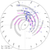 |
Fig. 1. Distribution on the Galactic plane of H II regions identified in the Urumqi λ6 cm survey with known distances. |
As listed in Table 2 and for some sources in Table 4, Paladini et al. (2003) collected many H II regions which were previously measured at λ6 cm. We made a comparison between the new results derived from the Urumqi data and those flux densities quoted in Paladini et al. (2003). We show the result in Fig. 2. The ratio is approximately 1 in general, proving the consistency, but the Urumqi flux densities are somewhat higher for those sources with higher flux densities. For some of the sources, one H II region seen in the Urumqi data can be resolved into several components, for example in Altenhoff et al. (1978) and Kuchar & Clark (1997). These components have to be added first, before the comparison. The angular resolution of the Urumqi survey is only slightly better than that of Altenhoff et al. (1970), but coarser than all the other eight surveys. Individual components of H II regions or underlying emission were possibly included in λ6 cm sources when the Urumqi data cannot resolve them (e.g. λ6 cm source G192.6−0.0 includes five H II regions: SH 2-254 to 258). The seeming overestimate of the Urumqi λ6 cm results is also caused by the fact that high angular resolution observations did not cover the entire, but only a part of the H II regions, for example G119.4−0.8 from Kuchar & Clark (1997).
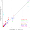 |
Fig. 2. Flux density comparison between the new λ6 cm measurements and previous λ6 cm results. |
There are some interesting newly identified objects in Table 4 and so in the following we first discuss a smaller number of objects in the WISE H II region catalogue, and then talk about many objects in the Paladini H II region catalogue.
4.1. Notes on some objects in the WISE H II region catalogue
WISE H II regions with sizes exceeding 8′ were used to search for a sample of λ6 cm extended H II regions. After excluding the small-diameter H II regions, 107 extended H II regions and H II region candidates whose flux densities can be reliably measured with the Urumqi λ6 cm data were catalogued and given in Table 4. Among these sources, more than 30 were found without counterparts in the WISE H II region catalogue. We show an example in Fig. 3. In the WISE 12 μm infrared image, 12 WISE H II regions (marked with white squares and blue dashed circles) are located in a 3 ° × 3° area centred at  ,
,  . Except for G125.606+2.099 (C-type) in the upper right corner, all the other WISE H II regions are Q-type WISE H II regions. They do not show up in either the CGPS λ21 cm or the Urumqi λ6 cm radio data as expected. The radio source G127.9+1.7, indicated by the red rectangle in Fig. 3, appears in both the CGPS and Urumqi images. Strong infrared emission is seen for some parts of this source in the WISE 12 μm image. G127.9+1.7 is not recorded in either the WISE H II region catalogue or the Paladini H II region catalogue. However, it is the true Galactic H II region DU 65 collected in Dubout-Crillon (1976). As supporting evidence, we displayed the Hα emission of G127.9+1.7 and the flat radio spectrum through TT-plot in the lower panels of Fig. 3 (TB ∼ νβ, β = α − 2).
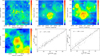 |
Fig. 3. Upper panels from left to right: WISE 12 μm, CGPS λ21 cm and Urumqi λ6 cm images centred at |


4.1.1. New H II regions
In addition to the missing known extended H II regions in the WISE H II region catalogue, a few new Galactic H II regions and H II region candidates are also discovered in the Urumqi λ6 cm survey. They are G68.4+0.2, G76.7−1.2, G94.4+2.7, G139.2−3.0, G139.9−2.0, G172.3+1.9 (H II region candidate), G186.7−4.0 (H II region candidate), G210.8−2.6 and G212.9−3.7. We show them in Figs. 4, 5 and 6. For G68.4+0.2, G76.7−1.2 and G94.4+2.7 it is difficult to compare the λ6 cm radio emission with the WISE 12 μm infrared emission due to the large difference in angular resolution. We extracted the 1′ resolution CGPS λ21 cm images and found that the associated infrared emission are not for the entire radio source but for partial shell- or ridge-like structures. The TT-plots confirmed their thermal origin. For the six remaining newly identified H II regions and H II region candidates, we found supporting evidence both in the TT-plot results and the associated Hα emission, except for G172.3+1.9 and G186.7−4.0. For G172.3+1.9, we did not obtain a reliable TT-plot result and for G186.7−4.0, which is not fully covered by the Effelsberg λ21 cm survey, the sensitivity of the Effelsberg λ11 cm data is not enough for a clear determination. The Hα image quality is not high in the south-east part of G172.3+1.9, but the data show a good correlation in the north-west part.
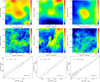 |
Fig. 4. New H II regions G68.4+0.2, G76.7−1.2 and G94.4+2.7 identified in the Sino-German λ6 cm survey. We show λ6 cm images and WISE 12 μm emission overlaid by CGPS λ21 cm total intensity in the upper and middle panels. We present their TT-plot results in the lower panels. |
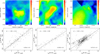 |
Fig. 5. Newly identified H II regions G139.2−3.0, G139.9−2.0 and G172.3+1.9. Hα emission overlaid by Urumqi λ6 cm total intensity contours are shown in the upper panel. The image quality of the south-east part of G172.3+1.9 is not good; however, correlation can be clearly recognised in the north-west part. TT-plot results are displayed in the lower panels. |
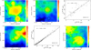 |
Fig. 6. Upper panels from left to right: λ6 cm image, Hα emission overlaid by Effelsberg λ11 cm total intensity and the TT-plot result for the new H II region G212.9−3.7. Lower panels from left to middle: Hα emission overlaid by Urumqi λ6 cm total intensity and the TT-plot result for the new H II region G210.8−2.6. Lower right panel: same as the lower left panel, but for G186.7−4.0. |
4.1.2. H II regions mistaken as SNRs
Some of the matched WISE H II regions challenge the SNR classification collected in the Green SNR catalogue (Green 2017). G11.183−1.063 is catalogued as a known WISE H II region, but also identified as a shell-type SNR (G11.1−1.0) with a spectral index of α ∼ −0.5 − −0.6 determined by the VLA λ90 cm (11.0 ± 0.3 Jy), the Southern Galactic Plane Survey (SGPS) and VLA λ21 cm (4.7 ± 0.8 Jy) and the Effelsberg λ11 cm (4.1 ± 0.4 Jy) data (Brogan et al. 2006). By adding the Urumqi λ6 cm measurement (3.40 ± 0.25 Jy), Sun et al. (2011b) found a spectral index of α = −0.41 ± 0.02. From Fig. 1 of Sun et al. (2011b), the spectral index fit for G11.1−1.0 strongly depends on the VLA λ90 cm result. Based on Effelsberg λ21 cm data, Reich et al. (1990b) reported a flux intensity of S21 cm = 5.17 ± 0.52 Jy closely agreeing with the previous SGPS/VLA result. The λ11 cm result of 4.082 Jy from the Effelsberg data is also consistent with the value reported by Brogan et al. (2006). The Urumqi λ6 cm result from Reich et al. (2014) is about 4.2 ± 0.2 Jy, a bit higher than that (3.40 ± 0.25 Jy) of Sun et al. (2011b). Using all these values except the λ90 cm result, we fit a new spectrum for G11.1−1.0 and found α = −0.16 ± 0.07, implying thermal emission. We show the comparison of the NVSS and WISE 12 μm data in Fig. 7, the radio and infrared emission of G11.1−1.0 have a very clear and good coincidence. Therefore, G11.1−1.0 seems to favour a H II region origin rather than a SNR identification.
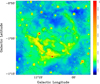 |
Fig. 7. WISE 12 μm image of G11.1−1.0 overlaid by NVSS 1.4 GHz radio continuum emission. |
A similar case was found for the source G20.4+0.1 ( ,
,  ) or G20.5+0.2 (
 ,
,  ). We found them to be duplicated in the Paladini H II region catalogue (see Sect. 4.2). Brogan et al. (2006) identified G20.47+0.16 to be a shell-type SNR with a spectral index of about α ∼ −0.4. However, in the WISE H II region catalogue, G20.482+0.169 is a K-type H II region with a similar size of a few arcmins. A flat radio continuum spectrum with α = −0.08 ± 0.09 was found in Sun et al. (2011b) and confirmed in this work (see Fig. 8, lower panel). These factors indicate that G20.47+0.16 is not a shell-type SNR, which agrees with the argument in Anderson et al. (2017).
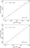 |
Fig. 8. TT-plots for G16.4−0.5 (upper panel) and G20.5+0.2 (lower panel) between Effelsberg λ21 cm data and Urumqi λ6 cm data. |
A further investigation is also needed for the source G16.4−0.5. Brogan et al. (2006) identified it as a SNR by revealing a partial shell structure and a steep spectrum with α = −0.7 ∼ −0.8. Sun et al. (2011b) derived a different spectrum with α = −0.26 ± 0.15. Using a TT-plot between the Effelsberg λ21 cm data and the Urumqi λ6 cm data, we obtained β = −1.99 ± 0.04 (see Fig. 8, upper panel). All these results do not support its shell-type SNR nature. The radio emission shown by the NVSS data is fragmented and difficult for a clear match to the WISE infrared emission. More sensitive high angular resolution radio observations are required to determine the shape and the nature of G16.4−0.5.
By optical data, G67.8+0.5, a WISE C-type H II region (G67.816+0.511) (Anderson et al. 2014) was identified as a SNR by Sabin et al. (2013). The currently available radio continuum data cannot yield a firm spectrum.
4.2. Notes on some objects in the Paladini H II region catalogue
We cross-matched the small-diameter H II regions in the Paladini catalogue listed in Table 2 with the WISE H II region catalogue. Only a few were found missing in the WISE H II region catalogue, for example G75.4−0.4 (see Fig. 9) and G137.4+0.2. They both show an arc-like structure in the WISE 12 μm and the NVSS 1.4 GHz images. Their radio spectra are flat and the infrared and radio emission are morphologically correlated.
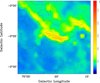 |
Fig. 9. WISE 12 μm image of the H II region G75.4−0.4 overlaid by NVSS 1.4 GHz radio continuum emission. |
Incorrect identifications are found in the Paladini H II region catalogue. Supernova remnants, planetary nebulae and steep-spectrum objects, likely extragalactic sources were noted. They are listed in Table 5.
78 misclassifications found in the Paladini H II region catalogue with the Urumqi λ6 cm data.
Seventeen surveys collected by Paladini et al. (2003) have overlapping regions with the Urumqi λ6 cm survey (see Table 1). These surveys were conducted from the late 1960s to the 1990s with various radio telescopes at seven different observing frequencies. We were aware of duplications when we noticed that the same remarks (e.g. Westerhout or Sharpless source names) were given to different but very nearby Paladini sources. Therefore, a self-intersection to the sample of the 777 Paladini objects within the λ6 cm survey area was made. Here we considered a coincidence when  , where d is the distance of the two centres of the Paladini sources and rp and
  are the radii of the two adjacent sources. Many duplicated identifications were found and we only discussed the ones which could be confirmed by the Urumqi λ6 cm data. Different angular resolutions in different surveys accounted for many of the cases. On the one hand, larger beam sizes include more emission and blend the peak position of the fitted centre. On the other hand, as mentioned above, H II regions identified in low angular resolution observations can be resolved into several discrete smaller H II regions in high angular resolution surveys. Different treatments of decimal places of the same source in different literature cause another kind of duplication. We discuss these duplications below. In the following, we use the abbreviation “PXXX” (No. XXX source in the Paladini catalogue) for a Paladini object.
-
P134 (010.3, −00.2) and P135 (010.3, −00.1): Both P134 and P135 are listed as individual point-like sources in the references in Table 2. The difference in designation very likely resulted from the different angular resolutions of the surveys. The similar flux densities achieved for P134 and P135 support that both P134 and P135 indicate the same radio source.
-
P155 (011.9, +00.7) and P156 (011.9, +00.8): The 4.9 GHz source list of W82 was based on A78. The coordinates of P155 and P156 are so close that none of the given reference surveys can resolve them. It is the radio counterpart of the optical H II region SH 2-38 (Sharpless 1959) as indicated in G70.
-
P164 (012.7, +00.3) and P166 (012.8, +00.4): P166 (Kuchar & Clark 1997; Altenhoff et al. 1978) is a single isolated radio object. No sources as strong as ∼2 Jy can be found in its vicinity. K97 obtained a flux density of ∼2.4 Jy, which is comparable with the results for P164 (SH 2-40, Altenhoff et al. 1970). A78 might have integrated a larger area and obtained a flux density exceeding 7 Jy. The optical image from the red plate of Digitised Sky Survey (Lasker et al. 1990) shows that SH 2-40 consists of several bright knots; this may cause the shift of central coordinates when observed with different angular resolutions.
-
P170 (013.2, +00.0) and P171 (013.2, +00.1): Based on the 45′′ resolution NVSS image, J181405-172832 with a flux density of S1.4 GHz = 2761.8 ± 85.2 mJy is the only strong source in this field. The high flux density obtained in various references might result from the low angular resolution which cannot resolve the influence of the ambient emission.
-
P179 (013.9, +00.2) and P180 (013.9, +00.3): NVSS J181435-164530 (S1.4 GHz = 3307.9 ± 120.0 mJy) is the only source that has a comparable flux density to that reported for both P179 and P180 in this area.
-
P189 (014.4, −00.7), P190 (014.4, −00.6) and P192 (014.5, −00.6): Based on the images from the Effelsberg λ11 cm data, only one point-like source was identified. Considering that P189, P190 and P192 share similar central coordinates and reported flux densities, they should represent the same source.
-
P199 (015.0, −00.7) / P200 (015.1, −00.9) / P203 (015.2, −00.8) / P204 (015.2, −00.6) and P201 (015.1, −00.7): From Table 2, it is clear that P199, P200, P203 and P204 are four individual components that are resolved by A78. For the low angular resolution observations of P199 and P201 (e.g. M67, A70), the individual components sum up. It is not clear why D80 gave high values for both P199 (344.5 Jy) and P201 (500 Jy).
-
P218 (016.9, +00.8), P219 (017.0, +00.8), P220 (017.0, +00.9) and P224 (017.1, +00.8): P218 (G70) and P219 (e.g. A70, R70) is a complex consisting of several components such as P218, P220 and P224 from K97. We measured the extended complex and listed it in Table 4.
-
P221 (017.0, +01.6) and P222 (017.0, +01.7): G17.0+1.6 (A70) and G17.0+1.7 (G70) were detected by observations with angular resolutions ≽8′. We retrieved the
 resolution Effelsberg λ11 cm image and cannot find point-like sources, but we do find an extended and elongated structure. We performed a TT-plot by using the Effelsberg λ21 cm data and the Urumqi λ6 cm data. The spectral index was found to be β = −2.11 ± 0.17 (β = α − 2), indicating a thermal nature. It is likely that the different designation of P221 and P222 comes from different fitted geometric centres.
 -
P232 (018.2, −00.3) and P230 (018.1, −00.3) / P231 (018.2, −00.4) / P233 (018.2, −00.2) / P235 (018.3, −00.4) / P236 (018.3, −00.3) / P239 (018.3, −00.4): SH 2-53 is a complex consisting of many individual portions as shown in the DSS red plate. The radio emission shown by F87 confirmed the existence of discrete components and extended emission. It is clear that A70, G70 and F87 measured the flux density of the entire structure, while P230, P231, P233, P235 (P239) and P236 from A78 are individual parts of SH 2-53. The low angular resolution flux density measurements may be affected by the nearby SNR G18.1−0.1.
-
P255 (019.2, +02.1) and P256 (019.2, +02.2): P255 is from the ∼11′ resolution data of A70. P256 comes from the 8′ resolution data of G70. The
 resolution Effelsberg λ11 cm data only show one source. However, this can be further resolved into two discrete sources in the NVSS data, with flux densities of ∼2 Jy and ∼1 Jy, respectively. The spectral index of each source cannot be found in Vollmer et al. (2010). The overall α21−11−6 = −0.52 ± 0.09 was obtained by using the Effelsberg λ21 cm, λ11 cm and the Urumqi λ6 cm data. No WISE counterpart was found for either of the sources. We put P255 and P256 into Table 5, which collects the mis-identifications of the Paladini H II region catalogue.
 -
P261 (019.7, −00.1) and P258 (019.6, −00.2) / P259 (019.6, −00.1) / P260 (019.7, −00.2): Based on the sources identified by A78, P258, P259 and P260 are three individual components that can be resolved by the Effelsberg 4.9 GHz observations. The low angular resolution measurements of G70, A70 and R70 summed the flux densities of discrete portions. K97 listed P258 and P259 as two separated sources with flux densities of 16.6 Jy and 15.2 Jy, respectively. This would double the flux density in this area and contradict the Effelsberg λ21 cm and the Urumqi λ6 cm measurements, unless they are multi-entries by K97.
-
P266 (020.2, −00.9), P267 (020.3, −00.9) and P268 (020.3, −00.8): These three entries share similar intrinsic source sizes of about ∼10′ and a consistent flux density of about 3 Jy. We list the source in Table 4 because its apparent size slightly exceeds 16′, which defines the small-diameter source of the Urumqi λ6 cm data.
-
P270 (020.4, +00.1) and P271 (020.5, +00.2): Both P270 and P271 match the position of the shell-type SNR G20.47+0.16 reported by Brogan et al. (2006). However, this may be a H II region (see detailed discussion in Sect. 4.1).
-
P292 (023.1, +00.5) and P293 (023.1, +00.6): As pointed out by A70 for P292 and G70 for P293, they are the same H II region SH 2-58.
-
P303 (023.9, +00.1), P304 (023.9, +00.2) and P305 (024.0, +00.2): The low angular resolution observations of A70 and G70 included the contributions of P303 and P305 by K97 and A78.
-
P317 (024.6, +00.5) and P318 (024.6, +00.6): Both P317 and P318 indicate the SNR G24.7+0.6. We listed them in Table 5.
-
P319/P320 (024.7, −00.2a/b) and P321 (024.7, −00.1): P319 and P320 are two sources extracted by K97 from radio recombination line observations of Lockman (1989). They are located at
 ,
,  and
and  ,
,  and therefore have the same abbreviation as G24.7−0.2. Paladini et al. (2003) gave the same flux density information (K97, A78, D80, W82 and W83) for both G24.7−0.2a and G24.7−0.2b, however, this seems incorrect. According to the central positions, the peak flux densities and the measured sizes of the sources of K97 and A78, G24.7−0.2a and G24.7−0.2b should have measured flux densities of 9.9 Jy and 3.2 Jy in K97 and 3.19 Jy and 1.42 Jy in A78, respectively. W82 and W83 measured the source centre at
  ,
,  and
and  ,
,  , which are closer to G24.7−0.2a rather than G24.7−0.2b. From the Effelsberg λ11 cm image, P321 should be the sum of P319 and P320. However, we cannot explain the high flux densities reported by A70 and G70.
 -
P333 (026.1, −00.1) and P334 (026.1, −00.0): By inspecting the NVSS and the Effelsberg λ11 cm images, we identified only one corresponding λ11 cm radio source with comparable flux densities.
-
P337 (026.5, +00.4) and P340 (026.6, +00.4): The same case as P333/P334.
-
P343 (027.3, −00.2) and P344 (027.3, −00.1): From the image of A78, G27.3−0.1 is a single point-like source on a curved ridge. The SNR G27.4+0.0 is nearby. The low angular resolution observations could possibly include the contribution of the unrelated emission and therefore overestimated the flux density. The 5 GHz observation of R70 measured a size of
 for G27.3−0.2. The elongation was possibly due to the inclusion of the point-like source itself and the underlying ridge.
 -
P362 (028.8, +03.5) and P363 (028.9, +03.5): Both P362 and P363 are marked as the H II region SH 2-64/W40. The transformation from RA–Dec to L–B coordinates for P363 actually gives
 ,
,  , the same as P362.
 -
P386 (030.7, −00.0) and P387 (030.8, −00.0): Both P386 and P387 are the H II region W43.
-
P398 (031.4, −00.3) and P399 (031.4, −00.2): By inspecting the low angular resolution images, P398 from A70 and P399 from B69 are the same point-like source. For P399, the transformation from RA–Dec to L–B coordinates results in
 ,
,  , which should lead to the same G-name as P398.
 -
P403 (031.8, +01.5), P404 (031.9, +01.3) and P405 (031.8, +01.4): G31.8+1.4 (P405) was reported to be the H II region SH 2-69 in F72 (see the Erratum of F72). P404 was marked as the H II region RCW 177 in A70. According to Dubout-Crillon (1976), SH 2-69 and RCW 177 share the same coordinates, implying the same identity. In the high angular resolution NVSS image, SH 2-69 shows a bubble-like structure. Regarding the low flux density measured for P403, K97 might only have measured a portion of the source.
-
P406 (032.1, −00.7) and P408 (032.2, +00.1): B69 gave an incorrect G-name for P406. According to the given RA–Dec coordinates, the centre of the source should be at
 ,
,  , very close to P408 at
  ,
,  . According to the NVSS image, only one matched point source is found in the field.
 -
P419 (034.3, +00.1) and P420 (034.3, +00.2): We compared the NVSS and the Effelsberg λ11 cm images. Considering the similar central positions and the flux densities reported for P419 and P420, they indicate the same radio source.
-
P421 (034.5, −01.1) and P422 (034.6, −01.1): The coordinates of P421 given by K97 is
 ,
,  . The G-name should be written as G34.6−1.1, the same as P422. The Effelsberg λ11 cm data only shows one source that is slightly extended in the field. No flux density information was found for P422 in B69.
 -
P431 (035.2, −01.8) and P432 (035.2, −01.7): For P431 and P432, the difference in coordinates is very small (see Table 2). Only one corresponding radio source is identified in the Effelsberg λ11 cm image.
-
P435 (035.3, −01.8) and P437 (035.4, −01.8): The same case as P431/P432.
-
P440 (035.6, −00.0), P441 (035.6, +00.1) and P442 (035.7, −00.0): P441, P442 and the high angular resolution measurements of P440 (e.g. A78, D80) are small discrete components, while the low angular resolution results of P440 from A70 and B69 cannot resolve individual parts but the entire structure.
-
P444 (036.3, −01.7), P445 (036.3, −01.6), P447 (036.4, −01.8) and P448 (036.4, −01.6): F72 reported that the 17′ diameter source P448 is the radio counterpart of the H II region SH 2-72 with the optical centre at
 ,
,  . P445 was marked by B69 as RCW 179 with a diameter of 15′, while P444 from A70 was also marked as RCW 179, having a size of 15′ × 16′. SH 2-72 and RCW 179 are the same H II region as indicated in Dubout-Crillon (1976). This is also supported by their similar flux densities and sizes. K97 identified two sources P444 and P447 with flux densities of 3.2 Jy and 0.8 Jy, respectively. They might be small individual components which are included in this extended structure.
 -
P449 (036.5, −00.2) and P450 (036.5, −00.1): The λ6 cm source at
 ,
,  is the only source that is close to P449 and P450. As supporting evidence, only one ring-like corresponding source is found in the NVSS data.
 -
P466 (037.8, −00.3), P468 (037.9, −00.4), P469 (037.9, −00.3): Based on the NVSS image, P468 (except for the result of R70) is a single point-like component which is included in the low angular resolution measurements of P466 and P469.
-
P477 (039.3, −00.1) and P478 (039.3, −00.0): Both P477 (W82) and P478 (A70, D70) are marked as NRAO 591.
-
P480 (039.5, +00.5) and P484 (039.6, +00.6): P480 and P484 have similar sizes and flux densities, as reported. Only one extended radio structure can be identified in the Effelsberg λ11 cm survey data.
-
P487 (039.9, −01.4), P488 (039.9, −01.3) and P494 (040.0, −01.3): We converted the RA–Dec coordinates reported by F72 to L–B coordinates for P487. The centre is
 ,
,  , very close to P488 centred at
  ,
,  . P494 was marked as RCW 182 by A70 and P487 was recognised as SH 2-74 by F72. By comparing the sizes and positions in Rodgers et al. (1960) and Sharpless (1959), RCW 182 and SH 2-74 indicate the same H II region.
 -
P490 (039.9, −00.2) and P491 (039.9, −00.1): P490 was identified by the
 resolution Parkes data (D70), while P491 was from the ∼11′ resolution NRAO data of A70. From a sharper view of the
  resolution Effelsberg λ11 cm image, we identified only one matching source at
  ,
,  .
. -
P501 (041.4, +00.4) and P505 (041.5, +00.4): Both P501 and P505 indicate the SNR G41.5+0.4. They are listed in Table 5.
-
P503 (041.5, +00.0) and P504 (041.5, +00.1): Considering the small differences in positions and flux densities, we identify P503 and P504 to be the same source after inspecting the NVSS and the Effelsberg λ11 cm image.
-
P511 (042.4, −00.3), P512 (042.5, −00.2) and P513 (042.6, −00.1): P512 from low angular resolution observations of A70 and D70 is reported to be an extended source. It contains small individual components that can be resolved in higher angular resolution images. P511 and P513 from K97 are two of the individual components inside P512.
-
P519 (043.3, +00.5) and P520 (043.4, +00.5): By converting RA–Dec to L–B coordinates for P519, we found that the G-name of P519 should be written as 043.4+00.5, the same as P520.
-
P524 (043.9, −00.8) and P525 (043.9, −00.7): We compared the NVSS and the Effelsberg λ11 cm images and found the λ11 cm source located at
 ,
,  is the only matching one.
 -
P529 (044.2, +00.1) and P531 (044.3, +00.1): The same case as P524/P525.
-
P530 (044.3, −00.4) and P532 (044.4, −00.3): The same case as P524/P525.
-
P540 (045.4, +00.1) and P541 (045.5, +00.1): Both P540 from D70 and P541 from A70 were marked as the radio source NRAO 601. Paladini et al. (2003) only listed one corresponding source for P541; we found the second component in A78/D80, W82 and W83. The sum of the two components agreed well with the results obtained from the low angular resolution observations (see Table 2).
-
P564 (049.5, −00.4) / P559 (049.3, −00.3), P561 (049.4, −00.5), P562 (049.4, −00.3), P563 (049.4, −00.2), P567 (049.6, −00.4): The low angular resolution observations of W51A, such as A70 for P564, smear out the individual structures (P559, P561, P562, P563, P567) that can be resolved by high angular resolution observations. It is not clear why the K97 measurements toward P561 and P564 both exceed 100 Jy, which result in a much larger flux density for W51A.
-
P570 (050.0, −00.1) and P571 (050.0, −00.0): The same case as P524/P525.
-
P578 (051.2, −00.1) and P579 (051.2, +00.1): P578 has a measured size of
 and a flux density of 37 Jy in R70, while A70 measured a similar size of 20′ × 20′ and comparable flux density of 35 Jy for P579. Considering the similar size and flux density, P578 and P579 should be the same source. It is embedded in a complex spanning over 1° (see Table 4). P576 and P580 are also included in this complex.
 -
P597 (054.1, −00.1) and P598 (054.1, −00.0): A70 suspected that the source P598 might be the steep-spectrum radio source 4C+18.57. From the NVSS image, 4C+18.57 is a single point-like source close to P597. These two objects cannot be resolved by the observation of A70. Thus, the measured flux density of P598 included the contribution of the H II region P597 and of 4C+18.57. It is not easy to obtain an accurate flux density for P597 with the Urumqi data due to the influence of the nearby SNR G54.4−0.3.
-
P605 (057.5, −00.3) and P606 (057.6, −00.3): The same case as P524/P525.
-
P619 (063.1, +00.4), P620 (063.2, +00.4) and P621 (063.2, +00.5): The same case as P524/P525. They are the H II region SH 2-90.
-
P624 (064.1, −00.5) and P626 (064.2, −00.5): Both P624 (F72) and P626 (A70) are marked as the H II region SH 2-93.
-
P632 (068.1, +00.9), P633 (068.1, +01.0) and P634 (068.2, +01.0): P633 from F72 and P634 from A70 are both reported as an extended source and marked as the H II region SH 2-98. They are incorporated in the λ6 cm extended H II region G68.20+1.05 in Table 4. From the high-resolution CGPS image, SH 2-98 is a ring-like structure with a diameter of about 25′. P632 from K97 is a bright, small-diameter (∼2′) source situated on the southern part of the ring. It can hardly be resolved in the low angular resolution observations such as A70 and F72. Therefore, the flux density measurements by A70 and F72 contain the entire ring structure and P632, while K97 only measure the point-like source. Due to influence of the ring structure, Reich et al. (2014) obtain a higher flux density for P632 than obtained by K97.
-
P636 (069.9, +01.5) and P637 (069.9, +01.6): In the λ6 cm image, P636 is a point-like source which is somehow confused by the radio emission in its north. Low angular resolution observations might overestimate the flux density. A good fit for the thermal radio spectrum was obtained through the Effelsberg λ21 cm, λ11 cm and the Urumqi λ6 cm data. However, it is strange that with the angular resolution similar to the Effelsberg λ21 cm data and the Urumqi λ6 cm data, S2.7 GHz = 14 Jy from A70 is so high.
-
P651 (074.8, +00.6) and P652 (074.8, +00.7): P651 from F72 and P652 from A70 were both proposed as the counterpart of the H II region SH 2-104. All the flux density estimates are consistent, except that by F72. With the angular resolution similar to the Urumqi data, the large flux density of 32.2 Jy is unclear.
-
P668 (078.0, +00.6) and P669 (078.1, +00.6): P668 is reported to be a point-like source with an intrinsic size of about 3′ in K97 and R70. This can be confirmed by the Effelsberg λ11 cm data. The source is isolated. W70 reported that P669 has a flux density of 18.5 Jy and a size of 9′ × 7′ after deconvolution. These results are difficult to explain.
-
P696 (078.9, +03.7) and P699 (079.0, +03.6): P699 was measured by W70 to have an intrinsic size of 28′ × 20′, while P696 has a larger source size of
 in R70. Considering the large size and the small difference between the central coordinates, P696 and P699 obviously indicate the same object.
 -
P721 (080.0, +00.8) and P722 (080.0, +00.9): P722 from K97 can be confirmed as a single point-like source by the Effelsberg λ11 cm data, which has a similar angular resolution. W70 obtained an intrinsic source size of 16′ × 16′ for P721, which encompasses the source of P722. The measured flux density of 17 Jy might result from the integration of a larger area.
-
P723 (080.0, +01.5) and P726 (080.1, +01.5): This duplication arises from different sizes found in different literature. For the same source P723, K97 reported an intrinsic source size of about 6′, but R70 reported
 5. For P726, W70 found 12′ × 22′. The
  angular resolution Effelsberg λ11 cm image shows an elongated structure rather than a point-like source. The different values for P723/P726 might result from the different areas selected for the flux density integration.
 -
P733 (080.4, +00.4) and P734 (080.4, +00.5): W70 measured an intrinsic size of 17′ × 22′ for P733, while R70 measured
 for P734. The two extended objects overlap and should be the same source. K97 obtained a much smaller size of about 5′ for P733. According to the Effelsberg λ11 cm image, which has a similar angular resolution to that of K97, K97 very probably measured only the compact central part of the source.
 -
P738 (080.8, +00.4) and P743 (080.9, +00.4): P743 was identified by K97 and R70 with a size of about 4′. It appears as a point-like source in the Effelsberg λ11 cm and Urumqi λ6 cm images. The flux density measurements by K97 and R70 can be clearly supported by the Effelsberg λ11 cm and the Urumqi λ6 cm data. P738 was identified by W70 with a much higher flux density of S2.7 GHz = 43.2 Jy and a much larger size of 17′ × 16′. We cannot explain the W70 result with the current data.
-
P741 (80.9, −00.2) and P742 (080.9, −00.1): High angular resolution observations of P741 and P742 region from the CGPS data shows a circular emission region (∼12′) with a bright source on its north-east edge. A thin shell structure (∼10′), which does not seem to be related, runs underneath the circular region. By overlaying the 87GB/GB6 sources on the image, it is possible that K97 only measured the upper bright part of the structure. At an angular resolution of about 10′ (e.g. R70 and W70), these structures can no longer be resolved but seen as a single point-like source.
-
P789 (097.5, +03.2) and P790 (097.6, +03.2): The same case as P524/P525.
-
P798 (104.6, +01.3) and P799 (104.6, +01.4): The H II region SH 2-135 has an oval shape with a size of 22′ × 15′ (Lynds 1965). K97 only measured the bright knots (P799) in its northern part, while F72 measured the entire structure (P798).
-
P812 (108.8, −01.0) and P813 (108.8, −00.9): Based on Sharpless (1959), SH 2-152 (
 ,
,  ) and SH 2-153 (
 ,
,  ) are two very close H II regions which the Urumqi λ6 cm observation cannot resolve. The flux density measurement by K97 may include both SH 2-152 and SH 2-153. The coordinate of P813 from W83 is
  ,
,  . The abbreviation should be the same as P812. W83 has a much better angular resolution than K97, who only measured SH 2-152.
 -
P817 (110.1, +00.0) and P818 (110.1, +00.1): Both P817 from F72 and K97 and P818 from W83 are the H II region SH 2-156.
-
P830 (115.0, +03.1) and P831 (115.0, +03.2): The same as the case of P524/P525.
-
P839 (119.4, −00.9) and P840 (119.4, −00.8): Based on the image of Effelsberg λ11 cm data, P839 from F72 is the H II region SH 2-173 with a circular shape and a bright western shell. From the coordinates given by K97 for P840, it is likely that K97 measured the western shell of SH 2-173 only.
-
P854 (136.4, +02.5) and P856 (136.5, +02.5): The same as the case of P524/P525.
-
P866 (151.6, −00.3) and P867 (151.6, −00.2): Both P866 from F72 and P867 from W83 were claimed to be the H II region SH 2-209, which consists of a northern component SH 2-209 N (
 ,
,  ) and a southern component SH 2-209 S (
 ,
,  ). F72 reported a lower central position, which might be influenced by SH 2-209 S.
 -
P869 (154.6, +02.4) and P870 (154.7, +02.4): The same as the case of P524/P525.
-
P887 (180.8, +04.0) and P888 (180.9, +04.1): P888 from F72 is thought to be the radio counterpart of the H II region SH 2-241. In the NVSS image, P888 mainly includes the source J060358+301522 (
 ,
,  ) and an area of diffuse emission in its south-east. It resembles the optical image of the H II region in the DSS red plate. P887 (
 ,
,  ) is catalogued by K97, but cannot be found in either the 87GB or the GB6 catalogue. We convolved the NVSS image to an angular resolution of
  , the same as K97. However, we failed to identify any source at
  ,
,  . The source J060358+301522 has a flux density of about S1.4 GHz = 140 mJy and a spectral index of α = −0.06 (Vollmer et al. 2010). It was also identified in the GB6 catalogue with a consistent flux density of S4.85 GHz = 158 mJy. Considering the similar flux density reported by K97 (SK97 = 0.164 Jy), it might be that P887 indicates the source NVSS J060358+301522, but is listed with wrong coordinates.
 -
P896 (192.1, +03.6) and P897 (192.2, +03.6): F72 reported that P896 is the H II region SH 2-253, whose optical centre is at
 ,
,  . It appears as an elongated diffuse structure both in the Effelsberg λ11 cm and in the Urumqi λ6 cm images. A similar optical morphology was seen in the DSS red plate. K97 gave a very small size and flux density for P897, which likely accounts for a part of the entire H II region.
 -
P905 (196.4, −01.7) and P906 (196.5, −01.7): The same as the case of P524/P525.
-
P909 (197.8, −02.4) and P910 (197.8, −02.3): From the NVSS image, a strong radio source is located at
 ,
,  (P910) and a few weak sources are visible around
  ,
,  . They show up as two radio sources in the
  resolution Effelsberg λ11 cm image. They cannot be separated in the
  resolution Urumqi λ6 cm data. The same case is expected for P909 from F72.
5. Summary
We identified and analysed H II regions from the Sino-German λ6 cm polarisation survey of the ∼2200 deg2 plane area. The small H II regions (apparent size < 16′) were obtained by cross-matches between the λ6 cm small-diameter sources of Reich et al. (2014), the Paladini radio H II region catalogue and the WISE infrared H II region catalogue, while the extended H II regions were found by overlaying the Paladini and WISE H II regions onto the Urumqi λ6 cm survey image and searching for coincidences by eye. The spectra of the chosen sources were examined by using the Effelsberg λ21 cm, λ11 cm, together with the Urumqi λ6 cm data. Finally, 401 H II regions were extracted from the λ6 cm survey. We listed their positions, λ6 cm flux densities and distances if available in Tables 2, 3 and 4.
Multi-frequency and multi-domain observations are important for H II region identification. The WISE H II region catalogue, being currently the largest, provides an excellent sample of small-diameter H II regions, but misses some extended H II regions as listed in Table 4. Among these ∼30 extended H II regions that were not present in the WISE H II region catalogue, 9 are revealed in this paper for the first time. In the Urumqi survey area, there are 78 mis-classifications and 76 pairs of duplicated identifications found in the Paladini H II region catalogue. The mis-classifications were mainly inherited from the literature from the 1970s. They are chosen by spectra check and/or by comparison with the SNR or PN catalogues. The duplications are mostly the results of the inclusion of both high and low angular resolution observations toward the same source.
G11.1−1.0, G20.4+0.1 and G16.4−0.5, were initially identified as SNRs by their shell-like appearance and steep radio continuum spectra (Brogan et al. 2006). However, the newly derived radio spectra of these three sources are all flat, which imply that their nature is thermal. Additionally, G11.1−1.0 (WISE H II region G11.183−1.063), G20.4+0.1 (WISE H II region G20.482+0.169) and G16.4−0.5 (WISE H II region G16.364−0.558) have all been identified as K-type, namely known H II regions in the WISE H II region catalogue and G11.1−1.0 shows well-correlated radio and infrared emission.
The λ6 cm survey data can be downloaded from www.mpifr-bonn.mpg.de/survey.html or http://zmtt.bao.ac.cn/6cm/surveydata.html
The λ6 cm sources at  ,
,  and
and  ,
,  are replaced by
  ,
,  and
and  ,
,  through refit. Two additional λ6 cm sources at
  ,
,  and
and  ,
,  determinded by Gaussian fitting are added in this work.
Acknowledgments
We would like to thank Dr. Thomas L. Wilson for the critical reading of the manuscript and the anonymous referee for the helpful comments. The Chinese authors are supported by the National Key R&D Program of China (NO. 2017YFA0402701), the Open Project Program of the Key Laboratory of FAST, NAOC, the Chinese Academy of Sciences, the National Natural Science foundation of China (11303035, 11503033) and the Partner group of the MPIfR at NAOC in the framework of the exchange programme between MPG and CAS for many bilateral visits. XYG acknowledges financial support from the CAS-NWO cooperation programme and Young Researcher Grant of National Astronomical Observatories, Chinese Academy of Sciences and the FAST FELLOWSHIP. The FAST FELLOWSHIP is supported by Special Funding for Advanced Users, budgeted and administrated by the Center for Astronomical Mega-Science, Chinese Academy of Sciences (CAMS). LGH is grateful for the support by the Youth Innovation Promotion Association CAS. The Digitized Sky Surveys were produced at the Space Telescope Science Institute under US Government grant NAG W-2166. The images of these surveys are based on photographic data obtained using the Oschin Schmidt Telescope on Palomar Mountain and the UK Schmidt Telescope. The plates were processed into the present compressed digital form with the permission of these institutions. The National Geographic Society – Palomar Observatory Sky Atlas (POSS-I) was made by the California Institute of Technology with grants from the National Geographic Society. The Wisconsin Hα Mapper and its Hα Sky Survey have been funded primarily by the National Science Foundation. The facility was designed and built with the help of the University of Wisconsin Graduate School, Physical Sciences Lab and Space Astronomy Lab. NOAO staff at Kitt Peak and Cerro Tololo provided on-site support for its remote operation. This publication makes use of data products from the Wide-field Infrared Survey Explorer, which is a joint project of the University of California, Los Angeles and the Jet Propulsion Laboratory/California Institute of Technology, funded by the National Aeronautics and Space Administration.
References
- Altenhoff, W. J., Downes, D., Goad, L., Maxwell, A., & Rinehart, R. 1970, A&AS, 1, 319 [NASA ADS] [Google Scholar]
- Altenhoff, W. J., Downes, D., Pauls, T., & Schraml, J. 1978, A&AS, 35, 23 [NASA ADS] [Google Scholar]
- Anderson, L. D., Bania, T. M., Balser, D. S., & Rood, R. T. 2011, ApJS, 194, 32 [NASA ADS] [CrossRef] [Google Scholar]
- Anderson, L. D., Bania, T. M., Balser, D. S., et al. 2014, ApJS, 212, 1 [NASA ADS] [CrossRef] [Google Scholar]
- Anderson, L. D., Armentrout, W. P., Johnstone, B. M., et al. 2015, ApJS, 221, 26 [NASA ADS] [CrossRef] [Google Scholar]
- Anderson, L. D., Wang, Y., Bihr, S., et al. 2017, A&A, 605, A58 [NASA ADS] [CrossRef] [EDP Sciences] [Google Scholar]
- Anderson, L. D., Armentrout, W. P., Luisi, M., et al. 2018, ApJS, 234, 33 [Google Scholar]
- Bania, T. M., Anderson, L. D., & Balser, D. S. 2012, ApJ, 759, 96 [NASA ADS] [CrossRef] [Google Scholar]
- Beard, M., & Kerr, F. J. 1969, Aust. J. Phys., 22, 121 [Google Scholar]
- Brogan, C. L., Gelfand, J. D., Gaensler, B. M., Kassim, N. E., & Lazio, T. J. W. 2006, ApJ, 639, L25 [NASA ADS] [CrossRef] [Google Scholar]
- Brunthaler, A., Reid, M. J., Menten, K. M., et al. 2009, ApJ, 693, 424 [NASA ADS] [CrossRef] [Google Scholar]
- Caswell, J. L., & Haynes, R. F. 1987, A&A, 171, 261 [NASA ADS] [Google Scholar]
- Choi, Y. K., Hachisuka, K., Reid, M. J., et al. 2014, ApJ, 790, 99 [NASA ADS] [CrossRef] [Google Scholar]
- Comerón, F., Pasquali, A., & Torra, J. 2006, A&A, 457, 553 [NASA ADS] [CrossRef] [EDP Sciences] [Google Scholar]
- Condon, J. J., & Kaplan, D. L. 1998, ApJS, 117, 361 [NASA ADS] [CrossRef] [Google Scholar]
- Condon, J. J., Broderick, J. J., & Seielstad, G. A. 1989, AJ, 97, 1064 [NASA ADS] [CrossRef] [Google Scholar]
- Condon, J. J., Griffith, M. R., & Wright, A. E. 1993, AJ, 106, 1095 [NASA ADS] [CrossRef] [Google Scholar]
- Condon, J. J., Cotton, W. D., Greisen, E. W., et al. 1998, AJ, 115, 1693 [NASA ADS] [CrossRef] [Google Scholar]
- Day, G. A., Warne, W. G., & Cooke, D. J. 1970, Aust. J. Phys. Astrophys. Suppl., 13, 11 [Google Scholar]
- Downes, D., Wilson, T. L., Bieging, J., & Wink, J. 1980, A&AS, 40, 379 [NASA ADS] [Google Scholar]
- Dubout-Crillon, R. 1976, A&AS, 25, 25 [Google Scholar]
- Felli, M., & Churchwell, E. 1972, A&AS, 5, 369 [NASA ADS] [Google Scholar]
- Fich, M., & Blitz, L. 1984, ApJ, 279, 125 [NASA ADS] [CrossRef] [Google Scholar]
- Finkbeiner, D. P. 2003, ApJS, 146, 407 [NASA ADS] [CrossRef] [Google Scholar]
- Foster, T., & Brunt, C. M. 2015, AJ, 150, 147 [NASA ADS] [CrossRef] [Google Scholar]
- Fragkou, V., Parker, Q. A., Bojičić, I. S., & Aksaker, N. 2018, MNRAS, 480, 2916 [NASA ADS] [CrossRef] [Google Scholar]
- Frew, D. J., Bojičić, I. S., & Parker, Q. A. 2013, MNRAS, 431, 2 [NASA ADS] [CrossRef] [Google Scholar]
- Fürst, E., Reich, W., Reich, P., Handa, T., & Sofue, Y. 1987, A&AS, 69, 403 [NASA ADS] [Google Scholar]
- Fürst, E., Reich, W., Reich, P., & Reif, K. 1990a, A&AS, 85, 691 [NASA ADS] [Google Scholar]
- Fürst, E., Reich, W., Reich, P., & Reif, K. 1990b, A&AS, 85, 805 [NASA ADS] [Google Scholar]
- Gao, X. Y., & Han, J. L. 2013, A&A, 551, A16 [NASA ADS] [CrossRef] [EDP Sciences] [Google Scholar]
- Gao, X. Y., Reich, W., Han, J. L., et al. 2010, A&A, 515, A64 [NASA ADS] [CrossRef] [EDP Sciences] [Google Scholar]
- Gao, X. Y., Han, J. L., Reich, W., et al. 2011, A&A, 529, A159 [NASA ADS] [CrossRef] [EDP Sciences] [Google Scholar]
- Goss, W. M., & Day, G. A. 1970, Aust. J. Phys. Astrophys. Suppl., 13, 3 [Google Scholar]
- Goss, W. M., & Shaver, P. A. 1970, Aust. J. Phys. Astrophys. Suppl., 14, 1 [Google Scholar]
- Graham, D. A., Haslam, C. G. T., Salter, C. J., & Wilson, W. E. 1982, A&A, 109, 145 [NASA ADS] [Google Scholar]
- Green, D. A. 2017, VizieR Online Data Catalog: VII/278 [Google Scholar]
- Handa, T., Sofue, Y., Nakai, N., Hirabayashi, H., & Inoue, M. 1987, PASJ, 39, 709 [NASA ADS] [Google Scholar]
- Harvey-Smith, L., Madsen, G. J., & Gaensler, B. M. 2011, ApJ, 736, 83 [NASA ADS] [CrossRef] [Google Scholar]
- Haynes, R. F., Caswell, J. L., & Simons, L. W. J. 1978, Aust. J. Phys. Astrophys. Suppl., 45, 1 [NASA ADS] [Google Scholar]
- Haynes, R. F., Caswell, J. L., & Simons, L. W. J. 1979, Aust. J. Phys. Astrophys. Suppl., 48, 1 [NASA ADS] [Google Scholar]
- Helfand, D. J., Velusamy, T., Becker, R. H., & Lockman, F. J. 1989, ApJ, 341, 151 [NASA ADS] [CrossRef] [Google Scholar]
- Honma, M., Bushimata, T., Choi, Y. K., et al. 2007, PASJ, 59, 889 [NASA ADS] [Google Scholar]
- Hou, L. G., & Han, J. L. 2014, A&A, 569, A125 [NASA ADS] [CrossRef] [EDP Sciences] [Google Scholar]
- Hou, L. G., Han, J. L., & Shi, W. B. 2009, A&A, 499, 473 [NASA ADS] [CrossRef] [EDP Sciences] [Google Scholar]
- Immer, K., Reid, M. J., Menten, K. M., Brunthaler, A., & Dame, T. M. 2013, A&A, 553, A117 [NASA ADS] [CrossRef] [EDP Sciences] [Google Scholar]
- Irabor, T., Hoare, M. G., Oudmaijer, R. D., et al. 2018, MNRAS, 480, 2423 [NASA ADS] [CrossRef] [Google Scholar]
- Kim, I.-J., Pyo, J., Jeong, W.-S., et al. 2018, ApJS, 238, 28 [NASA ADS] [CrossRef] [Google Scholar]
- Kuchar, T. A., & Clark, F. O. 1997, ApJ, 488, 224 [NASA ADS] [CrossRef] [Google Scholar]
- Landecker, T. L., Reich, W., Reid, R. I., et al. 2010, A&A, 520, A80 [NASA ADS] [CrossRef] [EDP Sciences] [Google Scholar]
- Lasker, B. M., Sturch, C. R., McLean, B. J., et al. 1990, AJ, 99, 2019 [NASA ADS] [CrossRef] [Google Scholar]
- Lockman, F. J. 1989, ApJS, 71, 469 [NASA ADS] [CrossRef] [Google Scholar]
- Lynds, B. T. 1965, ApJS, 12, 163 [NASA ADS] [CrossRef] [Google Scholar]
- Makai, Z., Anderson, L. D., Mascoop, J. L., & Johnstone, B. 2017, ApJ, 846, 64 [NASA ADS] [CrossRef] [Google Scholar]
- Mezger, P. G., & Henderson, A. P. 1967, ApJ, 147, 471 [NASA ADS] [CrossRef] [Google Scholar]
- Miszalski, B., Parker, Q. A., Acker, A., et al. 2008, MNRAS, 384, 525 [NASA ADS] [CrossRef] [Google Scholar]
- Miville-Deschênes, M., & Lagache, G. 2005, ApJS, 157, 302 [NASA ADS] [CrossRef] [Google Scholar]
- Moisés, A. P., Damineli, A., Figuerêdo, E., et al. 2011, MNRAS, 411, 705 [NASA ADS] [CrossRef] [Google Scholar]
- Moscadelli, L., Reid, M. J., Menten, K. M., et al. 2009, ApJ, 693, 406 [NASA ADS] [CrossRef] [Google Scholar]
- Oh, C. S., Kobayashi, H., Honma, M., et al. 2010, PASJ, 62, 101 [NASA ADS] [Google Scholar]
- Paladini, R., Burigana, C., Davies, R. D., et al. 2003, A&A, 397, 213 [NASA ADS] [CrossRef] [EDP Sciences] [Google Scholar]
- Parker, Q. A., Acker, A., Frew, D. J., et al. 2006, MNRAS, 373, 79 [NASA ADS] [CrossRef] [Google Scholar]
- Parker, Q. A., Bojičić, I. S., & Frew, D. J. 2016, J. Phys. Conf. Ser., 728, 032008 [CrossRef] [Google Scholar]
- Reich, P., & Reich, W. 1986, A&AS, 63, 205 [NASA ADS] [Google Scholar]
- Reich, P., Reich, W., & Fürst, E. 1997, A&AS, 126, 413 [NASA ADS] [CrossRef] [EDP Sciences] [Google Scholar]
- Reich, W. 1982, A&AS, 48, 219 [NASA ADS] [Google Scholar]
- Reich, W., Fürst, E., Haslam, C. G. T., Steffen, P., & Reif, K. 1984, A&AS, 58, 197 [NASA ADS] [Google Scholar]
- Reich, W., Fürst, E., Reich, P., Sofue, Y., & Handa, T. 1986, A&A, 155, 185 [NASA ADS] [Google Scholar]
- Reich, W., Fürst, E., Reich, P., & Reif, K. 1990a, A&AS, 85, 633 [NASA ADS] [Google Scholar]
- Reich, W., Reich, P., & Fürst, E. 1990b, A&AS, 83, 539 [NASA ADS] [Google Scholar]
- Reich, W., Sun, X. H., Reich, P., et al. 2014, A&A, 561, A55 [NASA ADS] [CrossRef] [EDP Sciences] [Google Scholar]
- Reid, M. J., Menten, K. M., Brunthaler, A., et al. 2009, ApJ, 693, 397 [NASA ADS] [CrossRef] [Google Scholar]
- Reifenstein, E. C., Wilson, T. L., Burke, B. F., Mezger, P. G., & Altenhoff, W. J. 1970, A&A, 4, 357 [NASA ADS] [Google Scholar]
- Rodgers, A. W., Campbell, C. T., & Whiteoak, J. B. 1960, MNRAS, 121, 103 [NASA ADS] [CrossRef] [Google Scholar]
- Russeil, D. 2003, A&A, 397, 133 [NASA ADS] [CrossRef] [EDP Sciences] [Google Scholar]
- Russeil, D., Adami, C., & Georgelin, Y. M. 2007, A&A, 470, 161 [NASA ADS] [CrossRef] [EDP Sciences] [Google Scholar]
- Rygl, K. L. J., Brunthaler, A., Reid, M. J., et al. 2010, A&A, 511, A2 [NASA ADS] [CrossRef] [EDP Sciences] [Google Scholar]
- Rygl, K. L. J., Brunthaler, A., Sanna, A., et al. 2012, A&A, 539, A79 [NASA ADS] [CrossRef] [EDP Sciences] [Google Scholar]
- Sabin, L., Parker, Q. A., Contreras, M. E., et al. 2013, MNRAS, 431, 279 [NASA ADS] [CrossRef] [Google Scholar]
- Sanna, A., Reid, M. J., Menten, K. M., et al. 2014, ApJ, 781, 108 [NASA ADS] [CrossRef] [Google Scholar]
- Sharpless, S. 1959, ApJS, 4, 257 [Google Scholar]
- Shi, W., Sun, X., Han, J., Gao, X., & Xiao, L. 2008, Chin. J. Astron. Astrophys., 8, 575 [NASA ADS] [CrossRef] [Google Scholar]
- Sieber, W., & Seiradakis, J. H. 1984, A&A, 130, 257 [NASA ADS] [Google Scholar]
- Sofue, Y., & Reich, W. 1979, A&AS, 38, 251 [NASA ADS] [Google Scholar]
- Su, H., Hurley-Walker, N., Jackson, C. A., et al. 2017, MNRAS, 465, 3163 [NASA ADS] [CrossRef] [Google Scholar]
- Suad, L. A., Cichowolski, S., Arnal, E. M., & Testori, J. C. 2012, A&A, 538, A60 [NASA ADS] [CrossRef] [EDP Sciences] [Google Scholar]
- Sun, X. H., Reich, W., Han, J. L., Reich, P., & Wielebinski, R. 2006, A&A, 447, 937 [NASA ADS] [CrossRef] [EDP Sciences] [Google Scholar]
- Sun, X. H., Han, J. L., Reich, W., et al. 2007, A&A, 463, 993 [NASA ADS] [CrossRef] [EDP Sciences] [Google Scholar]
- Sun, X. H., Reich, W., Han, J. L., et al. 2011a, A&A, 527, A74 [NASA ADS] [CrossRef] [EDP Sciences] [Google Scholar]
- Sun, X. H., Reich, P., Reich, W., et al. 2011b, A&A, 536, A83 [NASA ADS] [CrossRef] [EDP Sciences] [Google Scholar]
- Tasker, N. J., Condon, J. J., Wright, A. E., & Griffith, M. R. 1994, AJ, 107, 2115 [NASA ADS] [CrossRef] [Google Scholar]
- Taylor, A. R., Gibson, S. J., Peracaula, M., et al. 2003, AJ, 125, 3145 [NASA ADS] [CrossRef] [Google Scholar]
- Turtle, A. J., Pugh, J. F., Kenderdine, S., & Pauliny-Toth, I. I. K. 1962, MNRAS, 124, 297 [NASA ADS] [CrossRef] [Google Scholar]
- Vollmer, B., Gassmann, B., Derrière, S., et al. 2010, A&A, 511, A53 [NASA ADS] [CrossRef] [EDP Sciences] [Google Scholar]
- Wendker, H. J. 1970, A&A, 4, 378 [NASA ADS] [Google Scholar]
- Wilson, T. L., Mezger, P. G., Gardner, F. F., & Milne, D. K. 1970, A&A, 6, 364 [NASA ADS] [Google Scholar]
- Wink, J. E., Altenhoff, W. J., & Mezger, P. G. 1982, A&A, 108, 227 [NASA ADS] [Google Scholar]
- Wink, J. E., Wilson, T. L., & Bieging, J. H. 1983, A&A, 127, 211 [NASA ADS] [Google Scholar]
- Wu, Y. W., Sato, M., Reid, M. J., et al. 2014, A&A, 566, A17 [NASA ADS] [CrossRef] [EDP Sciences] [Google Scholar]
- Xiao, L., Han, J. L., Reich, W., et al. 2011, A&A, 529, A15 [NASA ADS] [CrossRef] [EDP Sciences] [Google Scholar]
- Xu, W. F., Gao, X. Y., Han, J. L., & Liu, F. S. 2013a, A&A, 559, A81 [NASA ADS] [CrossRef] [EDP Sciences] [Google Scholar]
- Xu, Y., Reid, M. J., Zheng, X. W., & Menten, K. M. 2006, Science, 311, 54 [NASA ADS] [CrossRef] [PubMed] [Google Scholar]
- Xu, Y., Li, J. J., Reid, M. J., et al. 2013b, ApJ, 769, 15 [NASA ADS] [CrossRef] [Google Scholar]
- Zhang, B., Zheng, X. W., Reid, M. J., et al. 2009, ApJ, 693, 419 [NASA ADS] [CrossRef] [Google Scholar]
- Zhang, B., Reid, M. J., Menten, K. M., et al. 2013, ApJ, 775, 79 [NASA ADS] [CrossRef] [Google Scholar]
- Zhang, B., Moscadelli, L., Sato, M., et al. 2014, ApJ, 781, 89 [NASA ADS] [CrossRef] [Google Scholar]
All Tables
Surveys compiled by Paladini et al. (2003) that overlap the λ6 cm survey region.
Small-diameter H II regions identified in the Urumqi λ6 cm survey by comparison with the Paladini H II region catalogue.
λ6 cm small-diameter H II regions that have WISE H II region counterparts but are not in the Paladini catalogue.
78 misclassifications found in the Paladini H II region catalogue with the Urumqi λ6 cm data.
All Figures
|
Fig. 1. Distribution on the Galactic plane of H II regions identified in the Urumqi λ6 cm survey with known distances. |
| In the text | |
|
Fig. 2. Flux density comparison between the new λ6 cm measurements and previous λ6 cm results. |
| In the text | |
|
Fig. 3. Upper panels from left to right: WISE 12 μm, CGPS λ21 cm and Urumqi λ6 cm images centred at |
| In the text | |
|
Fig. 4. New H II regions G68.4+0.2, G76.7−1.2 and G94.4+2.7 identified in the Sino-German λ6 cm survey. We show λ6 cm images and WISE 12 μm emission overlaid by CGPS λ21 cm total intensity in the upper and middle panels. We present their TT-plot results in the lower panels. |
| In the text | |
|
Fig. 5. Newly identified H II regions G139.2−3.0, G139.9−2.0 and G172.3+1.9. Hα emission overlaid by Urumqi λ6 cm total intensity contours are shown in the upper panel. The image quality of the south-east part of G172.3+1.9 is not good; however, correlation can be clearly recognised in the north-west part. TT-plot results are displayed in the lower panels. |
| In the text | |
|
Fig. 6. Upper panels from left to right: λ6 cm image, Hα emission overlaid by Effelsberg λ11 cm total intensity and the TT-plot result for the new H II region G212.9−3.7. Lower panels from left to middle: Hα emission overlaid by Urumqi λ6 cm total intensity and the TT-plot result for the new H II region G210.8−2.6. Lower right panel: same as the lower left panel, but for G186.7−4.0. |
| In the text | |
|
Fig. 7. WISE 12 μm image of G11.1−1.0 overlaid by NVSS 1.4 GHz radio continuum emission. |
| In the text | |
|
Fig. 8. TT-plots for G16.4−0.5 (upper panel) and G20.5+0.2 (lower panel) between Effelsberg λ21 cm data and Urumqi λ6 cm data. |
| In the text | |
|
Fig. 9. WISE 12 μm image of the H II region G75.4−0.4 overlaid by NVSS 1.4 GHz radio continuum emission. |
| In the text | |
Current usage metrics show cumulative count of Article Views (full-text article views including HTML views, PDF and ePub downloads, according to the available data) and Abstracts Views on Vision4Press platform.
Data correspond to usage on the plateform after 2015. The current usage metrics is available 48-96 hours after online publication and is updated daily on week days.
Initial download of the metrics may take a while.