| Issue |
A&A
Volume 622, February 2019
|
|
|---|---|---|
| Article Number | A133 | |
| Number of page(s) | 16 | |
| Section | Stellar structure and evolution | |
| DOI | https://doi.org/10.1051/0004-6361/201834400 | |
| Published online | 07 February 2019 | |
Flares in open clusters with K2⋆
I. M 45 (Pleiades), M 44 (Praesepe), and M 67
1
Leibniz-Institut für Astrophysik Potsdam, Germany
e-mail: This email address is being protected from spambots. You need JavaScript enabled to view it.
2
University of Washington, USA
e-mail: This email address is being protected from spambots. You need JavaScript enabled to view it.
Received:
8
October
2018
Accepted:
14
December
2018
Abstract
Context. The presence and strength of a stellar magnetic field and activity is rooted in a star’s fundamental parameters such as mass and age. Can flares serve as an accurate stellar “clock”?
Aims. To explore if we can quantify an activity-age relation in the form of a flaring-age relation, we measured trends in the flaring rates and energies for stars with different masses and ages.
Methods. We investigated the time-domain photometry provided by Kepler’s follow-up mission K2 and searched for flares in three solar metallicity open clusters with well-known ages, M 45 (0.125 Gyr), M 44 (0.63 Gyr), and M 67 (4.3 Gyr). We updated and employed the automated flare finding and analysis pipeline Appaloosa, originally designed for Kepler. We introduced a synthetic flare injection and recovery sub-routine to ascribe detection and energy recovery rates for flares in a broad energy range for each light curve.
Results. We collect a sample of 1761 stars, mostly late-K to mid-M dwarfs and found 751 flare candidates with energies ranging from 4 × 1032 erg to 6 × 1034 erg, of which 596 belong to M 45, 155 to M 44, and none to M 67. We find that flaring activity depends both on Teff, and age. But all flare frequency distributions have similar slopes with α ≈ 2.0−2.4, supporting a universal flare generation process. We discuss implications for the physical conditions under which flares occur, and how the sample’s metallicity and multiplicity affect our results.
Key words: methods: data analysis / stars: activity / stars: flare / stars: low-mass
The detected flare indices, the stellar parameters for M 44 and M 45, and a copy of Table 4 are available at the CDS via anonymous ftp to cdsarc.u-strasbg.fr (130.79.128.5) or via http://cdsarc.u-strasbg.fr/viz-bin/qcat?J/A+A/622/A133. We also published all flares we validated, and stellar parameters used for M 44 and M 45 in the same location.
© ESO 2019
1. Introduction
As stars age, their magnetic activity evolves. A magnetic dynamo should be at work within all stars with outer convection zones (Schatzman 1962). When the dynamic magnetic field in the interior reaches the stellar surface and interacts with the atmosphere, a variety of phenomena arise, including star spots, chromospheric emission, and flares (Parker 1979). Flares are magnetic reconnection events that lead to a change in field line topology and subsequent energy release (Priest & Forbes 2002). They reach from the chromosphere to the corona and emit electromagnetic energy in the form of both thermal and non-thermal emission in radio, hard and soft X-rays (> and ≤10 keV, respectively), UV, and white light (see Benz & Güdel 2010; Benz 2016, for detailed reviews). The amount of energy released during a stellar flare relative to the star’s luminosity can exceed the strongest solar flares and even temporarily amplify the optical stellar flux by orders of magnitude for cool dwarfs (Schaefer et al. 2000; Candelaresi et al. 2014). Flaring activity’s prospective observational availability and strong link to magnetic evolution has incited us to attempt to quantify it as a function of stellar age and mass.
Age, rotation, and magnetic activity are tightly interrelated by the concept of stellar dynamos (Noyes et al. 1984). Observational evidence for a relation between stellar rotation, mass, and age (Radick et al. 1987; Patten & Simon 1996; Queloz et al. 1998), and its theoretical backing (Mestel 1984; Kawaler 1988) gave rise to gyrochronology (Barnes 2003) – the age-dating of a single main sequence star from its mass and rotation period. Barnes (2010), Meibom et al. (2015) and Barnes et al. (2016) have found an unambiguous relation to hold for stellar ages from 0.6 Gyr (Hyades) up to about 4.3 Gyr (M 67) for solar type stars. However, this relation varies strongly with stellar mass (Barnes 2010; Van Saders et al. 2016). Additionally, the detectability of rotation periods in photometric data drops rapidly beyond solar ages, as noted by Esselstein et al. (2018). Secondary magnetic stellar age tracers such as chromospheric activity (Soderblom et al. 1991; Pace 2013; Lorenzo-Oliveira et al. 2016) or magnetic activity from Zeeman Doppler Imaging and Zeeman Broadening (Vidotto et al. 2014) are being explored but have not yet been developed into full blown age dating techniques.
Among these more or less expedient magnetic age tracers, flaring activity prospectively stands out with respect to practicability. In cool dwarfs, flares do not suffer from a lack of contrast to quiescent luminosity due to their ∼10 000 K blackbody spectrum (Hawley & Fisher 1992), and are observable in most common photometric bands (Benz & Güdel 2010). If flare processes are truly scale-invariant (Lacy et al. 1976; Shakhovskaya 1989) and have a sufficiently long cosmic activity timescale, a flaring-age clock may be calibrated for a broad range of stellar masses down to ultra-cool dwarfs (UCDs, Teff < 2900 K, Kirkpatrick et al. 1999) and take over when other age relations break down.
In accordance to dynamo theories, the flaring-age relation is expected to depend on stellar mass. In fact, Walkowicz et al. (2011) note that M dwarfs flare more often in white light (but are less energetic) than K dwarfs, and release more energy per time relative to their quiescent flux. However, at least for late-M dwarfs and UCDs, the relation seems weak (Paudel et al. 2018).
On the other hand, some constraints that limit the use of stellar age tracers may apply to a flaring clock as well: If rotation is the main driver of any magnetic activity, a flaring clock cannot be more precise than gyrochronology on an individual star. Short-term variations due to stellar activity cycles (Montet et al. 2017), breakdown of the relation in a certain age or mass range (e.g. Pace 2013; Paudel et al. 2018), or saturation of flaring activity above some critical Rossby number similar to what is observed in X-ray luminosity (Wright et al. 2011) could diminish the clock’s utility. Furthermore, a gyrochronology-type convergence of the flaring-age relation may not occur or occur later than in the case of rotation. Multiplicity of stellar systems affects our implications about the rotation-age relation both drawn from large samples (Douglas 2016; Douglas et al. 2017) and regarding individual systems’ evolution (Rebull et al. 2016). Similar arguments apply to flares. Metallicity influences magnetic activity (Gray et al. 2006; Karoff et al. 2018) and could affect flaring behaviour. A technical constraint is set by a target’s total available monitoring time relative to the flare frequency, in particular for ground based observations, but time-resolved photometric surveys like CoRoT (Auvergne et al. 2009), Kepler (Jenkins 2010) and the Transiting Exoplanetary Survey Satellite (TESS; Ricker et al. 2014) have begun to turn the tide.
Evidence for a measurable time scale for flaring activity in low-mass stars has accumulated during the last decade. Based on data from the Sloan Digital Sky Survey (SDSS; York et al. 2000), both Kowalski (2009) and Hilton et al. (2010) found that flaring M0–M6 dwarfs are preferentially found at lower Galactic heights than stars without notable flaring activity but with Hα emission, implying a flaring activity lifetime for these dwarfs that is shorter than the chromospheric activity lifetime. Doorsselaere et al. (2017) used Kepler photometry and rotation information from McQuillan et al. (2014) to find that flaring activity is a good predictor of rotation period, which makes a typical flaring activity timescale plausible. Moreover, Clarke et al. (2018) inferred a low intrinsic variability from a largely consistent relation between flaring activity level, rotation and age for pairs of coeval stars with similar masses in a sample of wide binaries found in Kepler archives.
In this work, we test if a mass-dependent flaring-age relation exists and can be inferred from flare statistics in open cluster (OC) photometry. OCs observed by Kepler’s follow up mission K2 (Howell et al. 2014) allow us to study large cohorts of coeval stars with a low spread in metallicity. We cover three of these objects, Pleiades (M 45, 0.125 Myr; Bell et al. 2012), Praesepe (M 44, 0.63 Gyr; Boudreault et al. 2012) and M 67 (4.3 Gyr; Dias et al. 2012), observed during the mission’s campaigns C4 and C5 (Sect. 2).
We detected flares as bright peaks in K2 time-domain photometry with the flare finding and analysis pipeline Appaloosa (Davenport 2016) (Sect. 3), using light curves (LCs) de-trended by Aigrain et al. (2016). Additional validation of flare candidates is obtained from an artificial signal injection and recovery sub-routine that characterizes individual LCs with respect to detection rate and energy recovery. We obtain flare frequency distributions (FFDs), determine flare activity indicators and analyse these as functions of Teff and age (Sect. 4). We discuss the role of the targets’ multiplicity and metallicity, and put the results in the context of flare physics and coronal heating mechanisms in Sect. 5.
2. Data
K2 time domain photometry was our source of flares, but the archived data needed to be cleared of both systematic effects and intrinsic variability before analysis. We collected cluster membership information as well as multiband photometry to derive spectral type and Teff for all targets that enabled us to group them by mass and age. We then estimated their luminosities to determine the energies that individual flares release. Each target was observed in 30 min cadence for up to 80 days yielding LCs in which we searched for flare signatures.
2.1. De-trended light curves
The Kepler (Koch et al. 2010) mission has produced a bounty of high precision photometric observations in the Cygnus-Lyra region since its launch in 2009. In 2013, two reaction wheels failed, and the mission had to be redesigned. In 2014, the follow-up mission K2 (Howell et al. 2014) began to conduct ∼80 days long observation campaigns nearby the ecliptic plane. Besides the reduced pointing accuracy, the main difference between Kepler and K2 data are additional instrumental artefacts that come along with the challenging task of keeping the satellite in place. Systematic errors occur on different time scales, among which a 6 h trend, associated with the spacecraft roll, is most prominent (Van Cleve et al. 2016). If the roll motion is not properly removed, its shape occasionally resembles flare signatures.
Two de-trending approaches achieve restoration of Kepler’s former precision to a very similar degree: the pixel-level de-correlation method developed by (Luger et al. 2016; EVEREST) and the Gaussian Process (GP) de-trending performed by (Aigrain et al. 2016; K2SC). Because their released data products already included LCs with removed periodic signals for campaigns C3 – C8 and C10, saving considerable computational effort, we opted for K2SC LCs (see example LC in Fig. 1).
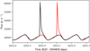 |
Fig. 1. 1.8 × 1034 erg superflare observed on EPIC 211119999 (M 45). Black: K2 PDC_SAP flux. Red: K2SC residual model with periodic trends added. The K2SC LC is offset by the dominant 0.58 d period for visual comparison. |
2.2. Open clusters in K2
There are about 16 OCs observed during K2 campaigns 0–18. They span a variety of ages from very young (M 21; 5 Myr; Piskunov et al. 2011) to some of the oldest known clusters, such as M 67 (Howell et al. 2014). As a rule of thumb, we expect a solar type star to exhibit a flare with 1034 erg once every 800 years (Maehara et al. 2012), but, in general, later type stars flare more frequently throughout the whole flare energy spectrum (Doorsselaere et al. 2017). By choosing very populous OCs, with >250 members each, where every object features 2MASS and/or Pan-STARRS band magnitudes (see Sect. 2.3 below) as well as de-trended K2SC LCs, we maximized the observation time. Aiming for a broad age range, M 45, M 44, and M 67 were selected for this initial study, so our sample covers ages from 125 Myr to 4.3 Gyr (Table 1).
Cluster sample, partly adopted from Howell et al. (2014).
M 45. We use the sample determined by Rebull et al. (2016), where membership probabilities are primarily based on recent proper motion studies (Bouy et al. 2015; Sarro et al. 2014; Lodieu et al. 2012). Rebull et al. (2016) inspected all ambiguous candidates on a case by case basis. We took the same subset of those candidates except that they excluded the targets without periodicities. This resulted in a set of high-confidence and lower-confidence members with 6 < Ks < 14.5, yielding a sample of 826 stars with K2 LCs. Lower-confidence means that all proper-motion studies confirmed it was an unambiguous member – as for high-confidence members – but single colour-magnitude diagrams (CMDs) placed the star off the respective sequence. We included these, because we later constructed our own CMDs and excluded certain targets by a similar criterion.
M 44. We use a sample from Kraus & Hillenbrand (2007), who analysed photometry and proper motions of ∼5 million objects to determine their memberships in different stellar populations. Douglas et al. (2014) selected 753 lower mass (<1.5 M⊙) and unsaturated (Kp > 9) stars from this survey with M 44 membership and K2 LCs, and added 41 known bright members not considered in the survey yielding a total of 794. We adopted their supplemented selection.
M 67. The sample was drawn from Gonzalez (2016), who, similar to Douglas et al. (2014) and Rebull et al. (2016), studied stellar variability in K2 LCs. They started with the sample used in the photometric survey by Nardiello et al. (2016), which they supplemented with other recent membership studies by (Yadav et al. 2008; proper motions) and (Geller et al. 2015; radial velocities). After checking for consistency in these works they assign, following Geller et al. (2015), a membership class to each object from which we only kept those classified as M (members), SM (single members) and BM (binary members), resulting in a working sample of 272 stars with K2 LCs.
From these three samples we removed targets that lacked multiband photometry and/or empirical template spectra, fell off the main sequence in g − r, r − i, and/or J − K CMDs, or were assigned spectral types hotter than F4.
2.3. Multiband photometry: Teff, R*, and excluded objects
To consistently ascribe approximate stellar spectra and ultimately luminosities to the stars we retrieved photometric data from either the Two Micron All Sky Survey (2MASS; Skrutskie et al. 2006) or the Panoramic Survey Telescope and Rapid Response System (Pan-STARRS) Data Release 1 (Chambers et al. 2016). For this, we matched the K2 sample by position with the Pan-STARRS catalogue, using the CDS XMatch tool1 to collect the Pan-STARRS grizy measurements (2MASS JHK magnitudes are already matched in EPIC), which we converted to SDSS grizy using Table 2 in Finkbeiner et al. (2016).
We used the available colour indices to derive Teff and R*, and eventually luminosities LKp, * that were required to determine individual released flare energies in the Kepler band (EKp, flare, see Sect. 2.5). We employed the synthetic SDSS and 2MASS colours from JHK and grizy bands, for solar metallicity standards (Pickles 1998) computed by Covey et al. (2007), and used the Modern Mean Dwarf Stellar Color and Effective Temperature Sequence, an up-to-date look-up table for spectral types, Teff, and R* derived from g − r, r − i, J − H, and H − K colours, compiled from the literature by Pecaut & Mamajek (2013)2.
The temperature accuracy σTeff in these two tables is heterogeneous for F4 to M9 dwarfs with median 75 K and ranging from 20 K to 220 K (see Table 2 for the correspondence of spectral types to Teff). The lowest accuracies are present for mid-K type stars. The majority of targets had all photometric measurements available. We adopted the median value from typically 3−4 calculated Teff. Due to recent findings, for example by Jackson et al. (2018), who conclude that radii for fast rotating M dwarfs in the Pleiades are underpredicted in stellar models by 14 ± 2%, we assumed an uncertainty in R* of ∼20%. This estimate also covered the spread in observed radii from Pecaut & Mamajek (2013).
Spectral type and Teff.
We excluded all likely non-main sequence, early spectral type, and foreground and background stars from the sample by examining the CMDs for g − r, r − i, and J − K colours. The union of objects that fell off the main sequence in these CMDs was rejected.
The final collection of targets mostly contains late-K to mid-M dwarfs and a few hotter stars. We divided our data in four sufficiently populated bins for stars below 4 000 K and otherwise considered the full sample.
2.4. Excluded data
A subset of data points from all LCs was excluded from further analysis to account for thruster firings and systematics which were not captured by the de-trending pipelines (see Table A.1 for an overview). CR flags were tracked but not removed. 24 severely saturated targets were removed from the sample. After the partial manual review of flare candidates we further excluded some LCs with anomalous variability and individual artefacts. A detailed description of excluded data and a full list of excluded LCs with high-energy artefacts is given in Appendix A.
2.5. Flare energies
Several individual flare parameters such as duration, amplitude, full width at half the maximum (FWHM), or released energy are typically used in flare statistics (see, e.g., Hawley et al. 2014; Yang et al. 2017, 2018). However, in long cadence LCs, duration and amplitude are subject to large errors arising mostly from low time sampling (Yang et al. 2018). The flare energy, that is, the integration of the LC flux during a flare with the quiescent flux subtracted, is less severely affected by this.
Often, flares are described by a Tflare ≈ 9000−10 000 K (Hawley & Fisher 1992; Kretzschmar 2011; Shibayama et al. 2013) blackbody spectral energy distribution (SED). We followed Shibayama et al. (2013), and defined the projected stellar quiescent luminosity LKp, * and the flare luminosity in the Kepler band LKp, flare as
 (1)
(1)
and
 (2)
(2)
respectively, with Aflare being the area covered by the flaring region on the stellar surface, R* the stellar radius and RKepler the Kepler response function given in the Kepler instrument handbook (Van Cleve & Caldwell 2016). B* and Bflare correspond to the SEDs of the star and the blackbody curve of the flare with Tflare. The ratio of these luminosities yields the relative flare luminosity aKp, flare as obtained from the Kepler LC:
 (3)
Kowalski et al. (2013) measured strong variations in Tflare and flare spectra both between events and during the course of individual flares in several dMe stars, limiting the utility of the blackbody approximation. Additionally, they noted strong time-dependent line emission with a complicated relationship to the continuum. The Kepler flare energy EKp, flare is more tractable. Instead of bolometric flare luminosity we used the observed flare luminosity in the Kepler band LKp, flare (Eq. (2)) and obtain
(3)
Kowalski et al. (2013) measured strong variations in Tflare and flare spectra both between events and during the course of individual flares in several dMe stars, limiting the utility of the blackbody approximation. Additionally, they noted strong time-dependent line emission with a complicated relationship to the continuum. The Kepler flare energy EKp, flare is more tractable. Instead of bolometric flare luminosity we used the observed flare luminosity in the Kepler band LKp, flare (Eq. (2)) and obtain
 (4)
(4)
ED is defined as the area between the LC and the quiescent flux, that is, the integrated flare flux divided by the median quiescent flux F0 of the star, integrated over the flare duration (Hunt-Walker et al. 2012):
 (5)
(5)
Since it is measured relative to the quiescent star, ED is a quantity independent of calibration and distance. We note that by this approximation we miss at least the ∼27% of the continuum flare flux that resides in the U band relative to the total in UBVR (Hawley & Fisher 1992) and flux from emission lines that lie outside the Kepler band (see Kowalski et al. (2013) and references therein). As a consequence, EKp, flare should be considered a lower limit to the total released energy of the flare.
We calculated LKp, * as defined in Eq. (1) using spectra for FGKM stars computed by Yee et al. (2017). Including a parametrized spectrum mitigates errors arising from deviations from the blackbody assumption which becomes particularly relevant as we move to low-mass stars that have strong absorption features in the Kepler band along with an ever lower flux overall. Yee et al. (2017) provide empirical spectra for 3000−7000 K and 0.1−16 R⊙ main sequence and giant branch stars with an approximate accuracy of ±100 K and 10%, respectively, rendering them approximately as precise as the colour-temperature relations in Pecaut & Mamajek (2013). We used Empirical SpecMatch (SpecMatch-Emp3) as a tool to assign template spectra according to the stars’ spectral types. The stored spectra have high resolution (R ≈ 60 000) and high signal-to-noise ratios (S/N ≈ 150). The metallicities are centred around solar values with a standard deviation of ∼0.2 dex and maximum deviations of ±0.6 dex. We included the spectral information from derived R* and Teff to match a spectrum FTeff, R* to each star:
 (6)
(6)
3. Automated flare finding
Appaloosa is an open-source4 flare finding and analysis procedure written in Python by Davenport (2016) for Kepler LCs. The original version performs two successive steps: First, a model is built for the quiescent stellar brightness. Second, outliers that fulfil a number of detection criteria are analysed and stored in a flare candidate list.
We skipped the first step and employed K2SC LCs, designed by Aigrain et al. (2016) for K2 data instead, because they already equipped us with robust de-trending and variability removal (see Fig. 1). With K2SC LCs, we could treat the residual flux directly and approximate the quiescent flux by the median of all flux measurements.
Chang et al. (2015) suggest to check every flux outlier for three criteria to determine if it is part of a flare: Outliers from the residual LC are treated as candidates if they exceed thresholds N1 and N2, defined in terms of the LC’s variance σ, that is,
 (7)
(7)
 (8)
(8)
where fi and wi are the photometric flux and uncertainty at a given time i, f̄ and σ are the median value and the statistical uncertainty in a continuous observation period, as introduced by Chang et al. (2015) in their FINDFlare algorithm. Eqs. (7) and (8) define the first two criteria; the third criterion (N3) is the minimum number of consecutive data points that fulfil Eqs. (7) and (8). We required at least 3 consequent data points (N3 ≥ 3, that is, durations of ≥1.5 h) for a candidate detection for all outliers that exceed the threshold N2 = 4. We overrode Eq. (7) by choosing N2 > N1. For all candidates, the start and end times, and ED (see Eq. (5)) were extracted.
3.1. Flare finding efficiency
A variety of reasons can prevent a flare from being detected in a LC – an event can be lost in the noise, cut off at the end of a continuous observing period, or subjected to filter effects induced by the employed de-trending procedure. Due to the iterative nature of the flare finding procedure and the heterogeneity of LCs it is also not possible to assess the efficiency of the code analytically. We addressed this problem in a cause-neutral, empirical manner: We test Appaloosa’s flare recovery efficiency by injecting artificial signatures generated from a semi-analytical flare model derived from the active dMe star GJ 1243 (Davenport et al. 2014).
The synthetic events were introduced to a LC at different times with varying amplitude and duration while avoiding overlap with real flare signatures (Davenport 2016, see Fig. 2). The contaminated LC passed through the entire flare finding pipeline. A flare was then considered recovered if the flare peak time was contained within the start and end times of any resulting flare event candidate. After relating all successful and failed detections to each other, the recovery rate as a function of ED was returned. Paudel et al. (2018) used this procedure to determine a minimum flare energy detected by the algorithm. We additionally separated this quantity into detection probabilities for individual flare energies and introduced improvements to flare energy recovery and the parameter space covered by the injection routine. Details and examples are given in Appendix B.
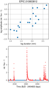 |
Fig. 2. Synthetic flare injection for EPIC 210803812 (M 45). Top panel: distribution of amplitudes and durations of synthetic flare injections. Bottom panel: representation of this distribution in the original K2SC de-trended LC. |
3.2. Post-detection treatment of flares
We specified a scheme for the post-detection treatment of individual flare candidates and the associated uncertainties in cumulative FFDs, illustrated in Fig. 3 on the example of M 44.
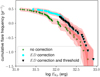 |
Fig. 3. Flare recovery and correction scheme for M 44 (3500−3749 K). Green crosses: all detected candidates, no cutoff at low probabilities, no correction for systematic underestimation of ED. Blue dots: all detected candidates, no cutoff at low probabilities, but corrected for systematic underestimation of ED. Black triangles: Final flare distribution after cutting off at the median detection thresholds for the bin and correcting for systematic underestimation of ED. Red shadows: One standard deviation uncertainties. |
As a first correction, we adjusted the recorded flare energies according to the energy recovery ratios obtained from synthetic flare injections. This typically shifted the distribution to higher energies in the diagram. In a second step, we rejected all flares with recovery probability below 20%, a number obtained from experimentation and manual vetting of candidates. We then bolstered the square-root growth of the Poissonian uncertainty by the strongly decreasing detection probability. As p decreases, the count uncertainty grew with p−1/2 resulting in correction factors up to 2.2.
Besides the uncertainties on the event counts and systematic errors on recovered flare EDs, we estimated the uncertainties for each flare’s EKp, flare (see overview in Table 3). Shibayama et al. (2013) report errors on their energy calculation to be around ±60%, which is consistent with our estimate of ∼65%. For most flares, uncertainties mainly stemmed from the uncertainty on Teff(colour) and R*, or Lbol,*, which could reach up to 80% while the uncertainty on ED is typically below 30% with the systematic error accounted for by the aforementioned ED correction.
Flare energy uncertainties.
All in all, the data set’s size and quality present a mixed picture. On one hand, the low time resolution of our LCs limits the investigations to high energy (super-)flares. The targets’ characterization in terms of Teff and Lbol, * is subject to large uncertainties, not least because of the observed departure of low mass stars from modern stellar models and the lack of standard stars for late-K type stars. These uncertainties propagated all the way through to EKp, flare. On the other hand, K2SC de-trended LCs nearly restored the original Kepler precision and provided good model fits to the systematic variations of individual LCs while preserving astrophysical signal. Ultimately, our synthetic flare injection procedure allowed us to evaluate the quality of each individual LC and additionally validated the detected candidates.
4. Results
We analyse if flaring activity depends on spectral type and age in late-K to mid-M dwarfs. After a short view on the total flare event counts we introduce activity indicators, that is, the flaring rate (FR), the energy released in flares (FA), and the power law fit exponent α and intercept β to the flare frequency distributions (FFDs). These indicators complement each other and can be linked to the underpinning astrophysical models as easy to interpret, direct activity measures. Remaining unresolved effects, such as metallicity and multiplicity of the investigated targets, are discussed in Sect. 5.
4.1. Flare counts
We did not find any flare candidates in M 67. The two other clusters yielded a final distribution of 751 flares in total, of which flares in M 45 contributed almost four times as many as M 44 despite comparable total observation durations. The vast majority of stars and flares were found in the range of late-K to mid-M spectral types. Using these flares, we constructed 5 FFDs per cluster (Fig. 4): four for flares on stars with Teff = 3000−4000 K divided in 250 K bins, and one for the total sample. The choice of bins reflects the balance between the relatively low spectral type resolution, the number of flares per bin and the comparability of bins. Too few flares were detected on stars hotter than 4000 K to allow for statistical interpretation.
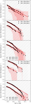 |
Fig. 4. Cumulative FFDs. Red lines: ODR fits. Red shadows: weighted Poissonian uncertainties on the frequency. Low energy thresholds are given in Table 4. Grey dotted lines indicate a power law with exponent −1 for comparison. |
At high energies we expect artefacts to contaminate the tail of the flare distributions. We inspected the LCs and TargetPixelFiles of all flares above 1034 erg using the interact function in lightkurve5 (Vinícius et al. 2018), a dedicated Kepler analysis package. As a result, we dropped three targets and 27 individual flares, listed in Table A.3 in Appendix A.
4.2. Flaring activity indicators
The contemporary approach to stellar flaring focuses on empirical studies rather than a robust theoretical description, so that it is unclear which indicator contains the most information about the process’ physical underpinning (Benz 2016). There is no single, generally accepted flaring activity indicator per star or group of stars. We consider four parameters that describe flaring activity and allow us to compare to previous work. The flare rate FR and the energy fraction released in flares FA measure how often flares occur and how strong flaring activity is relative to the quiescent stellar flux. The power law exponent α and intercept β can be obtained from fitting a line to the log-log representation of a FFD. α adds differential information to the average values covered by FA und FR. β depends on strongly on α but it can substitute for FR if α is assumed to be universal.
FR. Among statistical flaring activity indicators flare rates are the most directly accessible. By treating a sample of stars in a narrow temperature range as a single prototype star we can define a flaring rate FR as the number of flares ni recovered from all LCs i added up, divided by the sum of these LCs’ observation times ti:
 (9)
(9)
FR measures average flare frequency. We treat the uncertainty on FR as Poissonian in the total number of flares.
Flare luminosity. We define the average total energy released in flares per time as flare luminosity LKp, flare with
 (10)
(10)
The uncertainty is propagated from the uncertainties on individual EKp, flare.
FA. Alternative to the absolute LKp, flare we introduce a relative activity level measure where the total released energy is related to stellar bolometric luminosity Lbol, *. We consider, adapting the approach in Lurie et al. (2015), a flaring activity indicator FA that relates the total flare energy EKp, flare, tot released in the Kepler band relative to the estimated bolometric energy release ti ⋅ Lbol, *, i, where ti is the observation time of that star:
 (11)
(11)
N is the number of stars in a certain temperature bin. The uncertainty on FA is propagated in quadrature from the uncertainty on EKp, flare,i and Lbol, *, i. We use bolometric luminosity instead of Kepler luminosity because we relate flaring energy to the total energy of a star, but Kepler energy contains a different fraction of bolometric energy depending on spectral type. However, we implicitly assume that the fraction of flare energy released in the Kepler band does not depend on spectral type, assuming flare production is a universal process in this respect.
FFD. Using our synthetic flare injection procedure, we validated a total of 751 flare candidates, 596 in M 45, 155 in M 44. In Fig. 4, we divide the sample into 250 K bins and fit power laws to cumulative FFDs of stars with similar spectral type as well as to the entire samples in both clusters. We drop all flare candidates with EKp, flare below the median detection threshold in each bin. The cut accounts for the consequence of superimposing FFDs derived from LCs of different quality.
The occurrence rate of flares as a function of their energies, also termed flare frequency distribution (FFD; Lacy et al. 1976), can be written as
 (12)
(12)
In the log-log representation the above relation reads
![Mathematical equation: $$ \begin{aligned} \log N(E)\, \mathrm{d} E = [\log \beta -\alpha \log E]\, \mathrm{d} E. \end{aligned} $$](/articles/aa/full_html/2019/02/aa34400-18/aa34400-18-eq16.gif) (13)
(13)
In the corresponding cumulative distribution, a widely used representation in literature (see Audard et al. 2000; Hawley et al. 2014; Paudel et al. 2018, and references therein), the exponent becomes  . We fit the parameters given in Eq. (13) to the cumulative FFDs in Fig. 4. We used Orthogonal Distance Regression (ODR) to fit the line because it takes into account both uncertainties on flare rates and energies (see Hogg et al. 2010). The method yielded the best fit parameters
  and logβ, whose uncertainties we estimated using the delete-1 jackknife algorithm (Quenouille 1956).
Table 4 summarizes the resulting power law fit parameters for all FFDs. Overall, a power law slope α ≈ 2.0−2.4 is similar in most temperature bins and across both clusters. In the total sample and, marginally, in some of the 250 K bins, we notice a departure from the single power law at high energies.
FFDs: Results.
The values for β are typically dominated by α, as we can see in Fig. 5:
 (14)
(14)
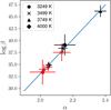 |
Fig. 5. Power law parameters to the FFDs, as in Eq. (12). Temperatures in the legend indicate Tmax. Black symbols: M 45. Red symbols: M 44. See also Table 4. Blue line: linear least square fit, see Eq. (14). |
If we attribute at least some of the deviation from a single power law to pixel saturation, we expect α to be lower. If we then assume α to be universal, we can perform a fit with α ≡ 2 and optimize only for the intercept logβ2. Figure 6 shows that β2 clearly depends on age but less on mass. Overall, β2 is consistent with the trends in FR.
4.3. Aging of FR, LKp, flare, and FA
FR, LKp, flare, and FA all decline with age (Fig. 7). In the time range from roughly ZAMS to 630 Myr flaring activity decreases faster with higher Teff. Stars in the 3000−3250 K bin follow the Skumanich t−1/2 law relatively closely for both indicators, hotter stars’ activity declines much faster. Above the highest detection threshold we can compare activity levels for fixed ages at the cost of higher uncertainties, as shown in Fig. 8, or alternatively in Figs. 9b–e. Figures 9b and c show that FR and LKp, flare are closely correlated. If the distribution from which flare energies are drawn is independent of the flaring rate, that is, if the flare generation process is universal on all activity levels, LKp, flare/FR will converge for large FR. We further discuss the question of universality in Sect. 5.
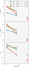 |
Fig. 7. Age dependent activity indicators. Colour and line shapes distinguish different Teff bins. Detection thresholds are derived from synthetic flare injections and averaged in each bin. For M 67, available upper limits are given with arrows. The highest energy we detect is ∼6 × 1034 erg. Top panel: flare rate FR; centre: absolute flare luminosity in the Kepler band LKp, flare. Bottom panel: flaring activity FA (see definitions in Sect. 4.2). Grey dotted lines indicate the Skumanich age−1/2 law for comparison. |
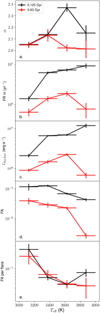 |
Fig. 9. Flaring activity measures for M 45 and M 44 as a function of Teff. Minimum energy threshold for LKp, flare, FA, and FR: 1.1 × 1033 erg. |
Our values of FR and FA confirm previous work that suggests an age dependence of flaring activity either from kinematic ages (Kowalski 2009; Hilton 2011), other OCs like intermediate-age M 37 compared to young clusters and the solar neighbourhood (Chang et al. 2015), or indirectly by showing that rotation, which is an age indicator itself, predicts flaring activity levels (Doorsselaere et al. 2017). Clarke et al. (2018) searched Kepler time-domain photometry of 33 equal-mass wide binaries for flares. They analysed the relative luminosity emitted in flares on individual stars and found that it was similar within each system: Stars that are alike in mass, metallicity and age exhibit similar magnetic activity levels. As our sample clusters all have similar, close to solar-like metallicities (see Table 1) and all stars in a cluster share approximately the same age, comparing stars with similar masses (Teff) between clusters should isolate the aging effect on flaring activity within the given uncertainties.
Recent work by Wright & Drake (2016) has shown that the saturation of X-ray emission LX with increasing Rossby numbers Ro (rotation period divided by convective turnover time) is not due to the lack of a tachocline by finding fully convective M dwarfs in the non-saturated regime of the LX(Ro) relation. Since flaring activity is tightly correlated with X-ray emission (Neupert 1968; Crosby et al. 1993; Hannah et al. 2011), our results can be interpreted in the context of the conclusions from Wright & Drake (2016): Stars follow a hotter-stars-deplete-faster rule for FR, LKp, flare, and FA in Fig. 8. M dwarfs, however, retain high activity levels for several hundred Myr, as Shkolnik & Barman (2014) found in X-ray, NUV, and FUV observations. This rule is consistent with the hotter-stars-spin-down-faster rule derived from stellar rotation studies (Barnes 2010), and supports the common view that rotation drives magnetic activity (Noyes et al. 1984). However, stellar magnetic fields modulate wind driven spin-down (Garraffo et al. 2018). We can see that the rotation-activity relationship is tight, but we also know that it is non-linear, both at young (Stauffer et al. 2016), and old (Van Saders et al. 2016) ages. For the young and probably fully convective stars, both the apparent saturation in FA, and the the lower flaring rates and LKp, flare hint at some regime change, possibly caused by the full convection boundary, and/or the transition from PMS to ZAMS to MS (see Fig. 8, blue lines).
4.4. Flaring activity indicators as a function of mass
We can confirm that M dwarfs flare more often than K dwarfs, as Walkowicz et al. (2011) found in Kepler Quarter 1 data (see also Candelaresi et al. 2014 and Doorsselaere et al. 2017). We find, for instance, that FR>4000 K/FR<4000 K is approximately 0.05 and 0.03 in M 45 and M 44, respectively. Our flaring rates are seemingly inconsistent with work from Davenport et al. (2012), who found that the time spent flaring increases for mid-M dwarfs compared to early-M type stars (see Fig. 9c). The sample in Davenport et al. (2012) was mostly composed of field stars so that the young age of our sample could explain the difference. As the authors measure flares in single epochs only, they derive flare luminosities instead of flare energies (see Davenport et al. (2012), Fig. 7). Assuming typical stellar flare durations of >103 s, the energy ranges in both works likely overlap in the logEbol, flare ∼ 33.5−34.5 erg range. As this is a somewhat narrow range, more detailed analysis may reveal that the distributions are disjoint, which is another possible explanation for the discrepancy.
FA per flare. A combination FA and FR is FA per flare that measures average flare energy. As opposed to FA and FR individually, FA per flare varies with Teff, but does not exhibit any significant age dependence (see Fig. 9d).
In late-M to L type dwarfs, it is believed that the ionization fraction decreases and atmospheric density increases leading to higher resistivity and decoupling of magnetic fields from the atmosphere (relaxation of the frozen-in condition), such that the random walk of surface magnetic loop footprints no longer twists energy into the field topology (Mohanty et al. 2002; Rodriguez-Barrera et al. 2015). Around 0.3 M⊙ (∼M3.5, Teff ≈ 3250 K; Hansen & Kawaler 1994; Delfosse et al. 2000) stars are thought transition to be fully convective, possibly altering their magnetic topology such that it impacts flare production (see, e.g., Reiners & Basri 2009). A 2750−3000 K bin we lack here would more certainly reside below the full convection boundary. These are both possible explanations, but we shall be cautious about interpretations that involve the absolute parameters of our targets. More generally, different starspot geometries (M. Gully-Santiago, priv. comm.) and varying magnetic field complexities (Garraffo et al. 2018) need to be considered in a complete picture.
5. Discussion
5.1. Time evolution of the power law slopes
We found values of the FFD power law slope α ≈ 2.0−2.4 with no apparent trend with age or mass. The underlying flare production process appears universal on all considered stars. This conclusion is not trivial.
Shakhovskaya (1989) concluded in her seminal work that flaring activity may be a function of age and that this effect originates in a change in surface magnetic field as the stars spin down over time. She found values for α ∼ 1.6 in M 44 and ∼1.8−2.0 in M 45 red dwarfs. More recently, Paudel et al. (2018) used kinematic ages of ten UCDs to discover a weak trend towards shallower α in stellar flaring activity for older ages.
An evolution towards a shallower slope along with an overall decline in FA could be read as follows: Although the overall magnetic energy of a star dissipates over time, the surface magnetic field topology evolves such that longer buildup periods of magnetic stress can occur, caused by slower surface convection and/or rotation. This allows the production of more strong flares relative to weak ones6. A description of the concrete physical model should involve, besides basic atmospheric parameters like density and temperature with their respective effects on ionization fractions, considerations of mass loss via flare associated cornal mass ejections (Drake et al. 2013; Alvarado-Gómez et al. 2018) and field complexity levels on observed bimodal spin-down modes, which are a topic of current research and theoretical studies by themselves (Barnes 2010; Newton et al. 2016; Garraffo et al. 2018).
5.2. Flares as coronal heating mechanisms in late-K to mid-M dwarfs
We found α ⪆ 2 for all temperatures and ages in our results, so it seems possible that flares present the main coronal heating mechanism. Since the outset of statistical flare studies, the energy distributions of flares are most frequently described by power laws (Lacy et al. 1976). The function’s exponent, that is, the slope α in the log-log representation, is highly relevant for our understanding of stellar coronae. Flares have been proposed as coronal heating mechanisms for M dwarfs early by Doyle & Butler (1985), who found X-ray luminosity to be correlated with the average UV energy released in flares. If α ≥ 2, the total energy released in flares can be arbitrarily high (Güdel et al. 2002). On the Sun, flare energies can be as low as 1026 erg in microflares (Shimizu 1995)7. Given a sufficiently steep distribution, one can imagine very low energy flares to be the main coronal heating mechanism. For α < 2, the highest energy flares contribute most to the total flare energy release and would occur too rarely to be responsible for the quiescent coronal temperature.
Numbers found in literature all revolve around the value of 2: Güdel et al. (2003) observed AD Leo (dMe3.5) in EUV and soft X-ray and found α = 2−2.5, Davenport et al. (2012) constrained α to be around 2 in M0–M6 dwarfs in red-optical and NIR in the SDSS and 2MASS photometric surveys. Lurie et al. (2015) determined α ≈ 2 for two dMe5 dwarfs, Gizis (2017) found α = 1.8 ± 0.2 for an M8 dwarf, and Paudel et al. (2018) studied time domain photometry of 10 L dwarfs in K2 data and concluded that α < 2 for the vast majority of investigated LCs.
Given the proximity of our results to the critical value, and the inconclusive results in other work, the question has to remain open, at least for stars other than the Sun.
5.3. Departures from the power law relation in FFDs
Flare production is a self-similar process with respect to released energy because we find the FFDs to follow a power law in a broad energy range across different spectral types and stellar ages. A break in or a deviation from this power law would reflect a change in the underlying physics.
A single power law is not always a good fit to our data, as one can see from the full sample FFDs for both clusters in the bottom row in Fig. 4. Such deviations have already been noticed in single target FFDs, for example by Hawley et al. (2014) and Davenport (2016). Paudel et al. (2018) find a broken power law and a power law with an exponential cutoff at the highest energies a better fit to the FFDs of two L dwarfs in K2 LCs. Mullan & Paudel (2018) argue that there could be more than one flare generating regime, that is, that flares with small energies are fundamentally different from larger flares regarding, for example the size of the reconnecting magnetic loop. Gershberg (2005) notes that both an instrument’s sensitivity (saturation) and a maximum energy a star of a certain type can release, may contribute to the deviations they observed for solar type stars.
Assuming that such a maximum energy Emax, flare exists for late K to mid-M dwarfs, we can argue that the departure from a single power law is the superposition of several stars’ FFDs with different Emax, flare. However, in contrast to our FFDs, the deviations discovered in previous work are associated with individual targets’ FFDs. Paudel et al. (2018), Hawley et al. (2014) and Davenport (2016) found some but far from all single target FFDs to show this type of departure. An undetected multiplicity, which would create the required superposition of FFDs, offers one explanation to this conspicuity. Another resolution is also plausible: On a single star, multiple active regions may produce a deviation from a single power law. These regions generate flares independently following the same physical process. But each region can have a different Emax, flare. Emax, flare is limited by a fraction of the maximum magnetic energy available in it (Shibata et al. 2013) which in turn depends on the region’s size, as Maehara et al. (2017) suggest for the Sun and Sun-like stars, and on the regions’ geometry as we know from solar observations (Sammis et al. 2000). A third possibility is that an undetected stellar (Gao et al. 2016) or close-in planetary companion (Lanza 2012) adds a fundamentally different but morphologically similar flare generation process on top of the intrinsic stellar flare distribution.
However, to test this hypothesis or other physical interpretations, instrumental effects have to be entirely removed first. While our algorithm removed many low-probability flares on the low-energy side, some outliers resulted in a deviation from the fitted power law, which can likely in part be attributed to the heterogeneous detection thresholds determined by the synthetic flare injection procedure. At the high energy end, the deviations can also stem from artefacts and pixel saturation induced systematic errors in the flare energies, some of which we unveiled and removed (see Appendix A). As a result, the high-energy end of the distribution affects the slope for the entire sample, which would be shallower if we excluded them.
5.4. Metallicity
We expect metallicity to be a relevant parameter for flare activity studies, because it directly affects the atmosphere within which flaring takes place, but our sample can probably be treated as if metallicity was controled for.
On one hand, Gray et al. (2006) found that metal rich stars ([M/H] > −0.2) have a bimodal chromospheric activity distribution while lower metallicity stars show a single peaked spread. Karoff et al. (2018) suggested an effect of metallicity on stellar differential rotation and the underlying dynamo8. They point out that increasing the metallicity increases the opacity, which in turn will increase the temperature gradient. Then the criterion for convection will be satisfied deeper in the star (Schwarzschild 1906). Deeper convection zones lead to longer convective turnover times near the base of the outer convection zones (Brun et al. 2017). Stronger differential rotation, a key parameter in the classical αΩ-dynamo, is the consequence (Bessolaz & Brun 2011).
On the other hand, magnetic activity in wide binaries, that naturally have the same metallicities, is similar within the pairs, as Clarke et al. (2018) show for 33 equal-mass binaries found in Kepler photometry. Thus, the limitation of our OC sample to solar like metallicity clusters dashes joy with pain: We cannot offhand extrapolate the determined age-activity-mass-relation to higher or lower metallicities, but we can mostly exclude that the different activity levels observed in the clusters are an effect of metallicity rather than age: In our sample, M 45 has close to solar metallicity, while M 44 is even more metal-rich (see also Table 1; Netopil et al. 2016). Unfortunately, the evidence found by Karoff et al. (2018) does not allow us to precisely quantify the effect for M 44 because they only compare two solar-type stars. With respect to Gray et al. (2006) we can neglect the differences in metallicity because all of our studied clusters clearly fall into the metal-rich regime.
5.5. Multiplicity
A quantitative comparison of flaring activity in single and binary members is beyond the scope of this paper, but we note that multiplicity affects our derived activity levels and can cause the misattribution of individual flares to the primary.
Multiplicity is ubiquitous among solar-type and lower mass stars affecting ∼50% of all systems (Duquennoy & Mayor 1991; Fischer & Marcy 1992). Bouvier et al. (2001) observed a binary frequency of about ∼50%, independent of age of the cluster by comparing M 44, M 45 and the star forming 2 Myr old cluster IC 348 for G and K type stars. The frequency is lower for M dwarfs (42±9%; Fischer & Marcy 1992) due to the decreasing mass range for companions, and keeps declining towards lower masses, as Boudreault et al. (2012) found for the 0.07 < M⊙ < 0.45 range for M 44, but did not fall below ∼17% within uncertainties for any mass bin they studied. For M 67, Geller et al. (2015) estimated the binary frequency to be as high as 57 ± 4%. Thus, the binary fraction considerably increases the number of individual stars in all clusters for low mass stars, similarly for M 44 and M 45, and even more notably in M 67, where higher mass stars prevail. The effects on both the total activity level and the flare energy distributions are twofold:
Firstly, the true FR and FA become lower, as the true number of stars and hence the cumulative observation time is significantly higher than the number of targets.
Secondly, energies of flares in unresolved binaries are underestimated, regardless of whether they occur on the larger or smaller star, because their EDs are measured relative to the quiescent luminosity of the whole system, but are multiplied only by the luminosity of the large companion that dominates the colour indices, while it should be the sum of both (see Eq. (4)).
The misattribution implies a shift of flaring activity levels to cooler stars within the 3000−4000 K range. It also implies an additional systematic offset to the location of the full convection boundary as may be marked by flares, which would reside at apparently higher spectral types. The dependence of magnetic activity on the presence of close companions may also affect flaring activity measurements, as discussed by Gao et al. (2016).
6. Summary and conclusions
Using K2SC de-trended Kepler/K2 LCs we investigated the flaring activity of three solar metallicity OCs, the ZAMS cluster M 45, intermediate age M 44 and solar age M 67, a total of more than 250 years of cumulative observation time at 30 min cadence from 1761 targets, mostly late-K and early- to mid-M dwarfs. Pan-STARRS and 2MASS multiband photometry yielded Teff and radii of individual stars, using solar metallicity standards (Pickles 1998), computed by Covey et al. (2007), and colour-temperature relations from Pecaut & Mamajek (2013). From these we derived quiescent luminosities and the Kepler band energies of flares detected by the flare finding and analysis pipeline Appaloosa (Davenport 2016).
We improved Appaloosa’s performance using GP Regression de-trended and variablity cleared LCs from Aigrain et al. (2016) instead of raw data. We introduced a synthetic flare injection and recovery routine to characterize long cadence K2SC de-trended LCs of heterogeneous quality. Over 9 million artificial flare signatures were injected and recovered. They yielded both ED-dependent detection thresholds and correction factors to the sampling induced systematic energy underestimation.
We found 751 flare candidates with EKp, flare ranging from 4 × 1032 erg to 6 × 1034 erg in two clusters, of which 596 belong to M 45 and 155 to M 44. We detected no flare candidates in M 67. We saw that both flare rates (FR) and energy released relative to bolometric luminosity (FA) substantially decline with age for late-K to mid-M dwarfs and follow a hotter-stars-deplete-faster rule. For cooler stars the mass dependence was weak. FA per flare did not show any age dependence and was consistently varying with mass in both clusters.
Our findings back previous suggestive evidence that a flaring-temperature-age relation exists. Although we did not find an age dependence in the FFD power law exponent α, we observed a distinct age dependence for various other activity measures that could prove to be useful age-dating techniques for low-mass stars, complementing existing methods. The lack of any trend in α suggests the universality of the flare production process across a broad range of masses, presumably below the full convection boundary. If α is universal, the power law intercept β2 can serve as another age-dependent activity measure.
Our results are at least valid for stars with solar or close to solar metallicities. We acknowledge that unresolved multiplicity causes misattribution of flares to the primaries, and an overestimation of flaring activity overall.
Assuming that our FFDs can be described by single power laws for all flare energies, it remains unclear if flares can be the main coronal heating mechanism because the power law exponents α we found were close to and above the critical value of 2. A single power law was not always a good fit to the FFDs, although it described the distributions in most individual temperature bins well. Pixel saturation effects at the FFDs’ high-energy ends could have caused such deviations. Alternatively, a high energy flaring limit that varies among stars could have produced the broken power law by superimposing their FFDs.
In addition to M 45, M 44 and M 67, K2 has endowed us with months of continuous monitoring of several OCs, spanning a range of ages from PMS to solar age. We will expand the analysis described in this paper to these targets in an upcoming project, and explore the effects of multiplicity and metallicity on the gears of a stellar flaring “clock”.
MacDonald & Mullan (2013), Feiden & Chaboyer (2013), and many others are working to pin down how magnetic activity affects modern stellar evolution. A comprehensive description of flaring activity as a function of age, which we attempted to approach here, may be one of the bottlenecks in our evolution models of exoplanetary atmospheres (Johnstone et al. 2015).
The updated version used here is 2018.03.22. It includes results from Kirkpatrick et al. (2011), Dieterich et al. (2014), Eker et al. (2015), Filippazzo et al. (2015), Benedict et al. (2016), Leggett et al. (2015), Schneider et al. (2015), Patel et al. (2014), West et al. (2011), Dahn et al. (2017) and Kaltcheva et al. (2017).
The argument works vice versa as well but with shorter buildup periods of magnetic stress that can no longer occur. This allows the production of fewer lower energy flares relative to stronger ones.
We do not consider nanoflares here, because they are produced by a different mechanism than classical flares (Benz 2016).
Here, Karoff et al. (2018) only discuss the classical, tachocline-dependent dynamo paradigm.
Acknowledgments
We are grateful to the anonymous referee for their constructive suggestions that significantly improved our interpretation of the results. We also wish to thank Sydney Barnes, Meetu Verma, and Jens Fischer for helpful comments and support. This research made use of pandas (McKinney 2010); Astropy, a community-developed core Python package for Astronomy (Astropy Collaboration et al. 2013); NumPy (Van Der Walt et al. 2011); and matplotlib, a Python library for publication quality graphics (Hunter 2007). This research also used the cross-match service provided by CDS, Strasbourg. Some of the data presented in this paper were obtained from the Mikulski Archive for Space Telescopes (MAST). STScI is operated by the Association of Universities for Research in Astronomy, Inc., under NASA contract NAS5-26555. This paper includes data collected by the Kepler/K2 mission. Funding for the Kepler mission is provided by the NASA Science Mission directorate. We made use of data products from the Two Micron All Sky Survey, which is a joint project of the University of Massachusetts and the Infrared Processing and Analysis Center/California Institute of Technology, funded by the National Aeronautics and Space Administration and the National Science Foundation. The Pan-STARRS1 Surveys (PS1) and the PS1 public science archive have been made possible through contributions by the Institute for Astronomy of the University of Hawaii, the Pan-STARRS Project Office, the Max-Planck Society and its participating institutes, the Max Planck Institute for Astronomy, Heidelberg and the Max Planck Institute for Extraterrestrial Physics, Garching, The Johns Hopkins University, Durham University, the University of Edinburgh, the Queen’s University Belfast, the Harvard-Smithsonian Center for Astrophysics, the Las Cumbres Observatory Global Telescope Network Incorporated, the National Central University of Taiwan, the Space Telescope Science Institute, the National Aeronautics and Space Administration under Grant No. NNX08AR22G issued through the Planetary Science Division of the NASA Science Mission Directorate, the National Science Foundation Grant No. AST-1238877, the University of Maryland, Eotvos Lorand University (ELTE), the Los Alamos National Laboratory, and the Gordon and Betty Moore Foundation. JRAD is supported by an NSF Astronomy and Astrophysics Postdoctoral Fellowship under award AST-1501418.
References
- Aigrain, S., Parviainen, H., & Pope, B. J. S. 2016, MNRAS, 459, 2408 [NASA ADS] [Google Scholar]
- Alvarado-Gómez, J. D., Drake, J. J., Cohen, O., Moschou, S. P., & Garraffo, C. 2018, ApJ, 862, 93 [NASA ADS] [CrossRef] [Google Scholar]
- Astropy Collaboration, (Robitaille, T. P., et al.) 2013, A&A, 558, A33 [NASA ADS] [CrossRef] [EDP Sciences] [Google Scholar]
- Audard, M., Gudel, M., Drake, J. J., & Kashyap, V. L. 2000, ApJ, 541, 396 [NASA ADS] [CrossRef] [Google Scholar]
- Auvergne, M., Bodin, P., Boisnard, L., et al. 2009, A&A, 506, 411 [NASA ADS] [CrossRef] [EDP Sciences] [Google Scholar]
- Barnes, S. A. 2003, ApJ, 586, 464 [NASA ADS] [CrossRef] [Google Scholar]
- Barnes, S. A. 2010, ApJ, 722, 222 [NASA ADS] [CrossRef] [Google Scholar]
- Barnes, S. A., Weingrill, J., Fritzewski, D., Strassmeier, K. G., & Platais, I. 2016, ApJ, 823, 16 [NASA ADS] [CrossRef] [Google Scholar]
- Bell, C. P. M., Naylor, T., Mayne, N. J., Jeffries, R. D., & Littlefair, S. P. 2012, MNRAS, 424, 3178 [NASA ADS] [CrossRef] [Google Scholar]
- Benedict, G. F., Henry, T. J., Franz, O. G., et al. 2016, AJ, 152, 141 [NASA ADS] [CrossRef] [Google Scholar]
- Benz, A. O. 2016, Liv. Rev. Sol. Phys., 14, 2 [Google Scholar]
- Benz, A. O., & Güdel, M. 2010, ARA&A, 48, 241 [NASA ADS] [CrossRef] [Google Scholar]
- Bessolaz, N., & Brun, A. S. 2011, ApJ, 728, 115 [NASA ADS] [CrossRef] [Google Scholar]
- Boudreault, S., Lodieu, N., Deacon, N. R., & Hambly, N. C. 2012, MNRAS, 426, 3419 [NASA ADS] [CrossRef] [Google Scholar]
- Bouvier, J., Duchêne, G., Mermilliod, J.-C., & Simon, T. 2001, A&A, 375, 989 [NASA ADS] [CrossRef] [EDP Sciences] [Google Scholar]
- Bouy, H., Bertin, E., Sarro, L. M., et al. 2015, A&A, 577, A148 [NASA ADS] [CrossRef] [EDP Sciences] [Google Scholar]
- Brun, A. S., Strugarek, A., Varela, J., et al. 2017, ApJ, 836, 192 [NASA ADS] [CrossRef] [Google Scholar]
- Candelaresi, S., Hillier, A., Maehara, H., Brandenburg, A., & Shibata, K. 2014, ApJ, 792, 67 [NASA ADS] [CrossRef] [Google Scholar]
- Chambers, K. C., Magnier, E. A., Metcalfe, N., et al. 2016, ArXiv e-prints [arXiv:1612.05560] [Google Scholar]
- Chang, S.-W., Byun, Y.-I., & Hartman, J. D. 2015, ApJ, 814, 35 [NASA ADS] [CrossRef] [Google Scholar]
- Clarke, R. W., Davenport, J. R. A., Covey, K. R., & Baranec, C. 2018, ApJ, 853, 59 [NASA ADS] [CrossRef] [Google Scholar]
- Covey, K. R., Ivezić, Ž., Schlegel, D., et al. 2007, AJ, 134, 2398 [NASA ADS] [CrossRef] [Google Scholar]
- Crosby, N. B., Aschwanden, M. J., & Dennis, B. R. 1993, Sol. Phys., 143, 275 [NASA ADS] [CrossRef] [Google Scholar]
- Dahn, C. C., Harris, H. C., Subasavage, J. P., et al. 2017, AJ, 154, 147 [NASA ADS] [CrossRef] [Google Scholar]
- Davenport, J. R. A. 2016, ApJ, 829, 23 [NASA ADS] [CrossRef] [Google Scholar]
- Davenport, J. R. A., Becker, A. C., Kowalski, A. F., et al. 2012, ApJ, 748, 58 [NASA ADS] [CrossRef] [Google Scholar]
- Davenport, J. R. A., Hawley, S. L., Hebb, L., et al. 2014, ApJ, 797, 122 [NASA ADS] [CrossRef] [Google Scholar]
- Delfosse, X., Forveille, T., Ségransan, D., et al. 2000, A&A, 364, 217 [NASA ADS] [Google Scholar]
- Dias, W. S., Monteiro, H., Caetano, T. C., & Oliveira, A. F. 2012, A&A, 539, A125 [NASA ADS] [CrossRef] [EDP Sciences] [Google Scholar]
- Dieterich, S. B., Henry, T. J., Jao, W.-C., et al. 2014, AJ, 147, 94 [NASA ADS] [CrossRef] [Google Scholar]
- Doorsselaere, T. V., Shariati, H., & Debosscher, J. 2017, ApJS, 232, 26 [NASA ADS] [CrossRef] [Google Scholar]
- Douglas, S. T. 2016, ApJ, 822, 47 [NASA ADS] [CrossRef] [Google Scholar]
- Douglas, S. T., Agüeros, M. A., Covey, K. R., et al. 2014, ApJ, 795, 161 [NASA ADS] [CrossRef] [Google Scholar]
- Douglas, S. T., Agüeros, M. A., Covey, K. R., & Kraus, A. 2017, ApJ, 842, 83 [NASA ADS] [CrossRef] [Google Scholar]
- Doyle, J. G., & Butler, C. J. 1985, Nature, 313, 378 [NASA ADS] [CrossRef] [Google Scholar]
- Drake, J. J., Cohen, O., Yashiro, S., & Gopalswamy, N. 2013, ApJ, 764, 170 [NASA ADS] [CrossRef] [Google Scholar]
- Duquennoy, A., & Mayor, M. 1991, A&A, 248, 485 [NASA ADS] [Google Scholar]
- Eker, Z., Soydugan, F., Soydugan, E., et al. 2015, AJ, 149, 131 [NASA ADS] [CrossRef] [Google Scholar]
- Esselstein, R., Aigrain, S., Vanderburg, A., et al. 2018, ApJ, 859, 167 [NASA ADS] [CrossRef] [Google Scholar]
- Feiden, G. A., & Chaboyer, B. 2013, ApJ, 779, 183 [NASA ADS] [CrossRef] [Google Scholar]
- Filippazzo, J. C., Rice, E. L., Faherty, J., et al. 2015, ApJ, 810, 158 [NASA ADS] [CrossRef] [Google Scholar]
- Finkbeiner, D. P., Schlafly, E. F., Schlegel, D. J., et al. 2016, ApJ, 822, 66 [NASA ADS] [CrossRef] [Google Scholar]
- Fischer, D. A., & Marcy, G. W. 1992, ApJ, 396, 178 [NASA ADS] [CrossRef] [Google Scholar]
- Gao, Q., Xin, Y., Liu, J.-F., Zhang, X.-B., & Gao, S. 2016, ApJS, 224, 37 [NASA ADS] [CrossRef] [Google Scholar]
- Garraffo, C., Drake, J. J., Dotter, A., et al. 2018, ApJ, 862, 90 [NASA ADS] [CrossRef] [Google Scholar]
- Geller, A. M., Latham, D. W., & Mathieu, R. D. 2015, AJ, 150, 97 [NASA ADS] [CrossRef] [Google Scholar]
- Gershberg, R. E. 2005, Solar-Type Activity in Main-Sequence Stars (New York: Springer Berlin Heidelberg) [Google Scholar]
- Gizis, J. E. 2017, ApJ, 845, 33 [NASA ADS] [CrossRef] [Google Scholar]
- Gonzalez, G. 2016, MNRAS, 459, 1060 [NASA ADS] [CrossRef] [Google Scholar]
- Gray, R. O., Corbally, C. J., Garrison, R. F., et al. 2006, AJ, 132, 161 [NASA ADS] [CrossRef] [Google Scholar]
- Güdel, M., Audard, M., Kashyap, V., Drake, J. J., & Guinan, E. F. 2002, in Stellar Coronae in the Chandra and XMM-Newton Era, eds. F. Favata, & J. J. Drake, ASP Conf. Ser., 277, 491 [NASA ADS] [Google Scholar]
- Güdel, M., Audard, M., Kashyap, V. L., Drake, J. J., & Guinan, E. F. 2003, ApJ, 582, 423 [NASA ADS] [CrossRef] [Google Scholar]
- Hannah, I. G., Hudson, H. S., Battaglia, M., et al. 2011, Space Sci. Rev., 159, 263 [NASA ADS] [CrossRef] [Google Scholar]
- Hansen, C. J., & Kawaler, S. D. 1994, Stellar Interiors. Physical Principles, Structure, and Evolution (New York: Springer Berlin Heidelberg) [Google Scholar]
- Hawley, S. L., & Fisher, G. H. 1992, ApJS, 78, 565 [NASA ADS] [CrossRef] [Google Scholar]
- Hawley, S. L., Davenport, J. R. A., Kowalski, A. F., et al. 2014, ApJ, 797, 121 [NASA ADS] [CrossRef] [Google Scholar]
- Hilton, E. J. 2011, PhD Thesis, University of Washington [Google Scholar]
- Hilton, E. J., West, A. A., Hawley, S. L., & Kowalski, A. F. 2010, AJ, 140, 1402 [NASA ADS] [CrossRef] [Google Scholar]
- Hogg, D. W., Bovy, J., & Lang, D. 2010, ArXiv e-prints [arXiv:1008.4686] [Google Scholar]
- Howell, S. B., Sobeck, C., Haas, M., et al. 2014, PASP, 126, 398 [NASA ADS] [CrossRef] [Google Scholar]
- Hunt-Walker, N. M., Hilton, E. J., Kowalski, A. F., Hawley, S. L., & Matthews, J. M. 2012, PASP, 124, 545 [Google Scholar]
- Hunter, J. D. 2007, Comput. Sci. Eng., 9, 90 [NASA ADS] [CrossRef] [Google Scholar]
- Jackson, R. J., Deliyannis, C. P., & Jeffries, R. D. 2018, MNRAS, 476, 3245 [NASA ADS] [CrossRef] [Google Scholar]
- Jenkins, J. M. 2010, ApJ, 713, L120 [NASA ADS] [CrossRef] [Google Scholar]
- Johnstone, C. P., Güdel, M., Stökl, A., et al. 2015, ApJ, 815, L12 [NASA ADS] [CrossRef] [Google Scholar]
- Kaltcheva, N., Golev, V., & Paunzen, E. 2017, PASP, 129, 114201 [NASA ADS] [CrossRef] [Google Scholar]
- Karoff, C., Metcalfe, T. S., Santos, Â. R. G., et al. 2018, ApJ, 852, 46 [NASA ADS] [CrossRef] [Google Scholar]
- Kawaler, S. D. 1988, ApJ, 333, 236 [NASA ADS] [CrossRef] [Google Scholar]
- Kirkpatrick, J. D., Reid, I. N., Liebert, J., et al. 1999, ApJ, 519, 802 [NASA ADS] [CrossRef] [Google Scholar]
- Kirkpatrick, D. J., Cushing, M. C., Gelino, C. R., et al. 2011, ApJS, 197, 19 [NASA ADS] [CrossRef] [Google Scholar]
- Koch, D. G., Borucki, W. J., Basri, G., et al. 2010, ApJ, 713, L79 [NASA ADS] [CrossRef] [Google Scholar]
- Kowalski, A. F. 2009, AJ, 138, 633 [NASA ADS] [CrossRef] [Google Scholar]
- Kowalski, A. F., Hawley, S. L., Wisniewski, J. P., et al. 2013, ApJS, 207, 15 [NASA ADS] [CrossRef] [Google Scholar]
- Kraus, A. L., & Hillenbrand, L. A. 2007, AJ, 134, 2340 [NASA ADS] [CrossRef] [Google Scholar]
- Kretzschmar, M. 2011, A&A, 530, A84 [NASA ADS] [CrossRef] [EDP Sciences] [Google Scholar]
- Lacy, C. H., Moffett, T. J., & Evans, D. S. 1976, ApJS, 30, 85 [NASA ADS] [CrossRef] [Google Scholar]
- Lanza, A. F. 2012, A&A, 544, A23 [NASA ADS] [CrossRef] [EDP Sciences] [Google Scholar]
- Leggett, S. K., Morley, C. V., Marley, M. S., & Saumon, D. 2015, ApJ, 799, 37 [NASA ADS] [CrossRef] [Google Scholar]
- Lépine, S., Hilton, E. J., Mann, A. W., et al. 2013, AJ, 145, 102 [NASA ADS] [CrossRef] [Google Scholar]
- Lodieu, N., Deacon, N. R., & Hambly, N. C. 2012, MNRAS, 422, 1495 [NASA ADS] [CrossRef] [Google Scholar]
- Lorenzo-Oliveira, D., Porto de Mello, G. F., Schiavon, R. P., et al. 2016, A&A, 594, L3 [NASA ADS] [CrossRef] [EDP Sciences] [Google Scholar]
- Luger, R., Agol, E., Kruse, E., et al. 2016, AJ, 152, 100 [Google Scholar]
- Lurie, J. C., Davenport, J. R. A., Hawley, S. L., et al. 2015, ApJ, 800, 95 [NASA ADS] [CrossRef] [Google Scholar]
- MacDonald, J., & Mullan, D. J. 2013, ApJ, 765, 126 [NASA ADS] [CrossRef] [Google Scholar]
- Maehara, H., Shibayama, T., Notsu, S., et al. 2012, Nature, 485, 478 [NASA ADS] [Google Scholar]
- Maehara, H., Notsu, Y., Notsu, S., et al. 2017, PASJ, 69 [Google Scholar]
- McKinney, W. 2010, in Proceedings of the 9th Python in Science Conference, eds. S. van der Walt, & J. Millman, 51 [Google Scholar]
- McQuillan, A., Mazeh, T., & Aigrain, S. 2014, VizieR Online Data Catalog: J/ApJS/211/24 [Google Scholar]
- Meibom, S., Barnes, S. A., Platais, I., et al. 2015, Nature, 517, 589 [NASA ADS] [CrossRef] [PubMed] [Google Scholar]
- Mestel, L. 1984, in Cool Stars, Stellar Systems, and the Sun, eds. S. L. Baliunas, & L. Hartmann (New York: Springer Berlin Heidelberg), 193, 49 [Google Scholar]
- Mohanty, S., Basri, G., Shu, F., Allard, F., & Chabrier, G. 2002, ApJ, 571, 469 [NASA ADS] [CrossRef] [Google Scholar]
- Montet, B. T., Tovar, G., & Foreman-Mackey, D. 2017, ApJ, 851, 116 [Google Scholar]
- Mullan, D. J., & Paudel, R. R. 2018, ApJ, 854, 14 [NASA ADS] [CrossRef] [Google Scholar]
- Nardiello, D., Libralato, M., Bedin, L. R., et al. 2016, MNRAS, 455, 2337 [NASA ADS] [CrossRef] [Google Scholar]
- Netopil, M., Paunzen, E., Heiter, U., & Soubiran, C. 2016, A&A, 585, A150 [NASA ADS] [CrossRef] [EDP Sciences] [Google Scholar]
- Neupert, W. M. 1968, ApJ, 153, L59 [NASA ADS] [CrossRef] [Google Scholar]
- Newton, E. R., Irwin, J., Charbonneau, D., et al. 2016, ApJ, 821, 93 [NASA ADS] [CrossRef] [Google Scholar]
- Noyes, R. W., Hartmann, L. W., Baliunas, S. L., Duncan, D. K., & Vaughan, A. H. 1984, ApJ, 279, 763 [NASA ADS] [CrossRef] [Google Scholar]
- Pace, G. 2013, A&A, 551, L8 [NASA ADS] [CrossRef] [EDP Sciences] [Google Scholar]
- Parker, E. N. 1979, Cosmical Magnetic Fields: Their Origin and Their Activity (New York: Oxford University Press) [Google Scholar]
- Patel, R. I., Metchev, S. A., & Heinze, A. 2014, ApJS, 212, 10 [NASA ADS] [CrossRef] [Google Scholar]
- Patten, B. M., & Simon, T. 1996, ApJS, 106, 489 [NASA ADS] [CrossRef] [Google Scholar]
- Paudel, R. R., Gizis, J. E., Mullan, D. J., et al. 2018, ApJ, 858, 55 [NASA ADS] [CrossRef] [Google Scholar]
- Pecaut, M. J., & Mamajek, E. E. 2013, ApJS, 208, 9 [NASA ADS] [CrossRef] [Google Scholar]
- Pickles, A. J. 1998, PASP, 110, 863 [CrossRef] [Google Scholar]
- Piskunov, A. E., Kharchenko, N. V., Schilbach, E., et al. 2011, A&A, 525, A122 [NASA ADS] [CrossRef] [EDP Sciences] [Google Scholar]
- Priest, E., & Forbes, T. 2002, A&ARv, 10, 313 [NASA ADS] [CrossRef] [Google Scholar]
- Queloz, D., Allain, S., Mermilliod, J.-C., Bouvier, J., & Mayor, M. 1998, A&A, 335, 183 [NASA ADS] [Google Scholar]
- Quenouille, M. H. 1956, Biometrika, 43, 353 [Google Scholar]
- Radick, R. R., Thompson, D. T., Lockwood, G. W., Duncan, D. K., & Baggett, W. E. 1987, ApJ, 321, 459 [NASA ADS] [CrossRef] [Google Scholar]
- Rebull, L. M., Stauffer, J. R., Bouvier, J., et al. 2016, AJ, 152, 113 [NASA ADS] [CrossRef] [Google Scholar]
- Reiners, A., & Basri, G. 2009, A&A, 496, 787 [NASA ADS] [CrossRef] [EDP Sciences] [Google Scholar]
- Ricker, G. R., Winn, J. N., Vanderspek, R., et al. 2014, J. Astron. Telesc. Instrum. Syst., 1, 014003 [Google Scholar]
- Rodriguez-Barrera, M. I., Helling, C., Stark, C. R., & Rice, A. M. 2015, MNRAS, 454, 3977 [NASA ADS] [CrossRef] [Google Scholar]
- Sammis, I., Tang, F., & Zirin, H. 2000, ApJ, 540, 583 [NASA ADS] [CrossRef] [Google Scholar]
- Sarro, L. M., Bouy, H., Berihuete, A., et al. 2014, A&A, 563, A45 [NASA ADS] [CrossRef] [EDP Sciences] [Google Scholar]
- Schaefer, B. E., King, J. R., & Deliyannis, C. P. 2000, ApJ, 529, 1026 [NASA ADS] [CrossRef] [Google Scholar]
- Schatzman, E. 1962, Ann. Astrophys., 25, 18 [Google Scholar]
- Schneider, A. C., Cushing, M. C., Kirkpatrick, J. D., et al. 2015, ApJ, 804, 92 [NASA ADS] [CrossRef] [Google Scholar]
- Schwarzschild, K. 1906, Nachr. Königlichen Ges. Wiss. Göttingen, 195, 41 [Google Scholar]
- Shakhovskaya, N. 1989, Sol. Phys., 121, 375 [NASA ADS] [CrossRef] [Google Scholar]
- Shibata, K., Isobe, H., Hillier, A., et al. 2013, PASJ, 65, 49 [NASA ADS] [Google Scholar]
- Shibayama, T., Maehara, H., Notsu, S., et al. 2013, ApJS, 209, 5 [NASA ADS] [CrossRef] [Google Scholar]
- Shimizu, T. 1995, PASJ, 47, 251 [NASA ADS] [Google Scholar]
- Shkolnik, E. L., & Barman, T. S. 2014, AJ, 148, 64 [NASA ADS] [CrossRef] [Google Scholar]
- Skrutskie, M. F., Cutri, R. M., Stiening, R., et al. 2006, AJ, 131, 1163 [NASA ADS] [CrossRef] [Google Scholar]
- Soderblom, D. R., Duncan, D. K., & Johnson, D. R. H. 1991, ApJ, 375, 722 [NASA ADS] [CrossRef] [Google Scholar]
- Stauffer, J., Rebull, L., Bouvier, J., et al. 2016, AJ, 152, 115 [NASA ADS] [CrossRef] [Google Scholar]
- Van Cleve, J. E., & Caldwell, D. A. 2016, Kepler Instrument Handbook (KSCI-19033-002) [Google Scholar]
- Van Cleve, J. E., Howell, S. B., Smith, J. C., et al. 2016, PASP, 128, 075002 [NASA ADS] [CrossRef] [Google Scholar]
- Van Der Walt, S., Colbert, S. C., & Varoquaux, G. 2011, Comput. Sci. Eng., 13, 22 [CrossRef] [Google Scholar]
- Van Saders, J. L., Ceillier, T., Metcalfe, T. S., et al. 2016, Nature, 529, 181 [NASA ADS] [CrossRef] [PubMed] [Google Scholar]
- Vidotto, A. A., Gregory, S. G., Jardine, M., et al. 2014, MNRAS, 441, 2361 [NASA ADS] [CrossRef] [Google Scholar]
- Vinícius, Z., Barentsen, G., Hedges, C., Gully-Santiago, M., & Cody, A. M. 2018, KeplerGO/lightkurve: Lightkurve v1.0b25 [Google Scholar]
- Walkowicz, L. M., Basri, G., Batalha, N., et al. 2011, AJ, 141, 50 [NASA ADS] [CrossRef] [Google Scholar]
- West, A. A., Morgan, D. P., Bochanski, J. J., et al. 2011, AJ, 141, 97 [NASA ADS] [CrossRef] [Google Scholar]
- Wright, N. J., & Drake, J. J. 2016, Nature, 535, 526 [NASA ADS] [CrossRef] [PubMed] [Google Scholar]
- Wright, N. J., Drake, J. J., Mamajek, E. E., & Henry, G. W. 2011, ApJ, 743, 48 [NASA ADS] [CrossRef] [Google Scholar]
- Yadav, R. K. S., Bedin, L. R., Piotto, G., et al. 2008, A&A, 484, 609 [NASA ADS] [CrossRef] [EDP Sciences] [Google Scholar]
- Yang, H., Liu, J., Gao, Q., et al. 2017, ApJ, 849, 36 [NASA ADS] [CrossRef] [Google Scholar]
- Yang, H., Liu, J., Qiao, E., et al. 2018, ApJ, 859, 87 [NASA ADS] [CrossRef] [Google Scholar]
- Yee, S. W., Petigura, E. A., & von Braun, K. 2017, ApJ, 836, 77 [NASA ADS] [CrossRef] [Google Scholar]
- York, D. G., Adelman, J., Anderson, Jr., J. E., et al. 2000, AJ, 120, 1579 [CrossRef] [Google Scholar]
Appendix A: Excluded data
Excluded data: Flagged data points.
Excluded data: Extremely saturated targets.
Cosmic ray contamination. Cosmic ray (CR) events occur randomly, possibly adding an offset to the flaring rate of a star because they may be mimicking flare signatures. Unlike the original Kepler mission, K2 does not identify and remove cosmic ray signals in optimal aperture due to the reduced calibration and photometric analysis pipelines. CRs in pixels collateral to optimal aperture, however, are flagged and can be used to extract information about the data quality. In Campaigns 0–11 a CR is flagged if the counts in a pixel exceed the 4σ limit compared to a rolling band median of five cadences. In our sample, CR flags made up ∼4−7% of all data points depending on the campaign. We note that from Campaign 11 on the threshold was increased to 7σ to minimize false detections triggered by K2’s roll motion9.
A CR hitting the optimal aperture or spilling signal into it from collateral pixels and signals stemming from flares are possibly ambiguous in long cadence data. Both produce a sudden increase in flux. A higher temporal resolution mitigates the problem: True flares can be identified by the characteristic shape of the flare signal with its impulsive rise and decline followed by a more gradual decay phase. For flares with durations shorter than ∼1.5 h, or 3 data points, K2 long cadence data do not resolve any of these features and we did not include any candidates with less than 3 consecutive data points in our analysis (i.e. N3 ≥ 3, see Sect. 3).
Excluded data: Rejected after manual inspection.
A CR induced flaring rate offset can vary, particularly when the spacecraft drifts and changes its attitude towards the Sun until it rotates again for a new campaign. Different campaigns and the relative position of the target on the CCD can play a role: The spacecraft may shield certain parts of the detector from CR impact better than others.
We acknowledged the possible CR contamination in our data but treated them as a statistical offset that affects all LCs in a similar manner: We interpret the similar amounts of CR flags we found in all OC samples (see Table A.1) to indicate comparability of the OCs. The weak trend may even reflect true flaring activity differences in the sample.
Thruster firings and field-wide systematics. We removed data points labelled as coinciding with the spacecraft’s thruster firings as well as their preceding and succeeding measurements that are often flagged as CRs. This procedure excluded 11−18% of all data points from the individual LCs (see Table A.1).
Even if the de-trending procedure removed most systematic effects from the LC, some may have remained undetected. To identify false positive detections, we compared all LCs and their respective flare candidate time to each other in order to find field-wide systematics. We assumed that flares occur randomly and rejected as precautionary measure all flare detections that were detected in more LCs simultaneously than this assumption would allow.
Saturated targets and artefacts. According to Van Cleve & Caldwell (2016), if the flux in a pixel exceeds the full well depth of 10093 DN by a factor <10, the detector response may still be linear if one considers the total flux in a sufficiently large aperture. We excluded 24 targets from our analysis, where the detected flare candidates exceeded this threshold, listed in Table A.2. Finally, we vetted the ∼100 most energetic flares by eye and excluded uncertain, clearly artificial signals or failed LCs from the results (see Table A.3).
Appendix B: Synthetic flare injection and recovery
Improvements to the routine. We carried out several enhancements to the original artificial flare injection sub-routine to improve the validity of the returned recovery rates. The original code injected 100 synthetic flares into a LC at once, a number too small to characterize the whole LC but too large to create mostly single and not superimposed events. We introduced an artificial flare grid in the amplitude-duration space and conducted more injections with fewer flares instead. We assumed that a LC’s properties are uniform throughout the campaign during which it was recorded. The convergence of the recovery probability distribution was a reasonable expectation because the flare finding procedure is deterministic, that is, the same fake flare infested LC yields the same recovered flares. We note that artificial flare injection cannot take care of false positive signals. We addressed the issue by manually vetting high-energy events, and comparing multiple LCs to identify field-wide systematics.
We could directly infer the recovery probability for the injected flare EDs. Observed flares’ EDs, however, are systematically underestimated in data with low time sampling (30 min) compared to 1 min cadence LCs, as Yang et al. (2018) found for Kepler data. We compared the injected with the recovered ED for every artificial flare. From the ratio, that is, the recovered share of the injected energy, we derived a correction factor that allowed us to ascribe both a more realistic flare energy and the corresponding recovery rate to each candidate (see Fig. B.1).
In summary, we obtained two ED-dependent corrections to the EDs and the recovered flare rates for each flare: an ED correction factor and a correction to the Poissonian count uncertainty, respectively. We accounted for the systematic energy underestimation on a LC by LC basis (Fig. B.1). Each LC obtained a unique flare recovery relation from the series of synthetic flare injections as a function of injected ED. This detection rate of synthetic events revealed the detection threshold for flares and provided a means to account for flares detected within the transition region by increasing the uncertainty on the detected number of flares accordingly (Fig. B.2).
For M dwarfs, Hawley et al. (2014) found clear evidence for an exponential distribution of flare amplitudes as a function of duration. We enabled users of Appaloosa to generate artificial flares generously covering this empirical parameter space (Fig. 2). The main advantage is a better coverage of the low-energy end of the expected flare distribution which is also most densely populated.
Realistic synthetic flare injections. Caution is recommended regarding the universality of injected flare shapes. Although the self-similarity of flares with different duration and amplitudes for a large parameter range is striking, the semi-analytical flare model used to generate synthetic events is derived from the flare distribution of a single star, GJ 1243 (Davenport et al. 2014), a bright dMe flare star in the northern sky (Lépine et al. 2013). Furthermore, Davenport et al. (2014) found a small portion (1.3%) of flares on that star that could only poorly be fitted by this single star model. The injection procedure was therefore tailored to characterize a LC’s quality with respect to the most common flares on GJ 1243. It could be extended to treat superpositions of classical flares, that is, multiflare events, that can amount to 15% of all events (Davenport et al. 2014) and are occasionally created, but complex shapes cannot be represented by the injections, although they can be recovered by the detection routine we employed here. We acknowledge that there is room for improvement in this respect.
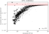 |
Fig. B.1. Example of recovered energy ratios from synthetic flare injections. Ratio of the originally injected ED recovered by Appaloosa in the K2SC de-trended long cadence LC for EPIC 210803812. The circle size represents the calculated relative uncertainty σED/ED. The red lines are placed at 100% (filled) and 110% (dashed) energy recovery, given for orientation. |
Light curve quality from synthetic flare injections. Relying on LCs alone for the detection of flare candidates required detailed quality assessment of each LC. We therefore injected and recovered 20 randomly distributed flares into every LC and repeated the process 300 times each using Appaloosa. Of these injections ∼5%, were dropped, because they were juxtaposed with more energetic events yielding more complex signatures. Consequently, ∼5700 synthetic flares injected into each LC – a total of more than 9 million events to cover all LCs – were used to retrieve information about their quality with respect to thresholds of detection, and systematic errors on energy recovery. For each cluster, this resulted in individual recovery rates based on the properties of the de-trended LCs, for example noise levels, time resolution, or variability time scales and magnitudes. Other properties may have been implicitly covered, because the procedure did not make any a priori assumptions about what affects flare signature detectability and to what degree. Overall, flare energies were systematically underestimated with significant uncertainties that become smaller with increasing energy (see Fig. B.1). Recovery rates typically exceed 80% as soon as some LC specific threshold for detection was exceeded, for example the time resolution limit. However, 100% recovery of both events and their energies was never achieved due to the cutoff of continuous observation periods (Fig. B.2).
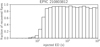 |
Fig. B.2. Recovery rate of classic flare events as a function of ED for EPIC 210803812. |
All Tables
All Figures
|
Fig. 1. 1.8 × 1034 erg superflare observed on EPIC 211119999 (M 45). Black: K2 PDC_SAP flux. Red: K2SC residual model with periodic trends added. The K2SC LC is offset by the dominant 0.58 d period for visual comparison. |
| In the text | |
|
Fig. 2. Synthetic flare injection for EPIC 210803812 (M 45). Top panel: distribution of amplitudes and durations of synthetic flare injections. Bottom panel: representation of this distribution in the original K2SC de-trended LC. |
| In the text | |
|
Fig. 3. Flare recovery and correction scheme for M 44 (3500−3749 K). Green crosses: all detected candidates, no cutoff at low probabilities, no correction for systematic underestimation of ED. Blue dots: all detected candidates, no cutoff at low probabilities, but corrected for systematic underestimation of ED. Black triangles: Final flare distribution after cutting off at the median detection thresholds for the bin and correcting for systematic underestimation of ED. Red shadows: One standard deviation uncertainties. |
| In the text | |
|
Fig. 4. Cumulative FFDs. Red lines: ODR fits. Red shadows: weighted Poissonian uncertainties on the frequency. Low energy thresholds are given in Table 4. Grey dotted lines indicate a power law with exponent −1 for comparison. |
| In the text | |
|
Fig. 5. Power law parameters to the FFDs, as in Eq. (12). Temperatures in the legend indicate Tmax. Black symbols: M 45. Red symbols: M 44. See also Table 4. Blue line: linear least square fit, see Eq. (14). |
| In the text | |
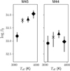 |
Fig. 6. Power law parameters to the FFDs, as in Eq. (12) with α ≡ 2. See also Table 4. |
| In the text | |
|
Fig. 7. Age dependent activity indicators. Colour and line shapes distinguish different Teff bins. Detection thresholds are derived from synthetic flare injections and averaged in each bin. For M 67, available upper limits are given with arrows. The highest energy we detect is ∼6 × 1034 erg. Top panel: flare rate FR; centre: absolute flare luminosity in the Kepler band LKp, flare. Bottom panel: flaring activity FA (see definitions in Sect. 4.2). Grey dotted lines indicate the Skumanich age−1/2 law for comparison. |
| In the text | |
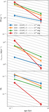 |
Fig. 8. Same as Fig. 7 but with equal detection thresholds for all Teff bins. |
| In the text | |
|
Fig. 9. Flaring activity measures for M 45 and M 44 as a function of Teff. Minimum energy threshold for LKp, flare, FA, and FR: 1.1 × 1033 erg. |
| In the text | |
|
Fig. B.1. Example of recovered energy ratios from synthetic flare injections. Ratio of the originally injected ED recovered by Appaloosa in the K2SC de-trended long cadence LC for EPIC 210803812. The circle size represents the calculated relative uncertainty σED/ED. The red lines are placed at 100% (filled) and 110% (dashed) energy recovery, given for orientation. |
| In the text | |
|
Fig. B.2. Recovery rate of classic flare events as a function of ED for EPIC 210803812. |
| In the text | |
Current usage metrics show cumulative count of Article Views (full-text article views including HTML views, PDF and ePub downloads, according to the available data) and Abstracts Views on Vision4Press platform.
Data correspond to usage on the plateform after 2015. The current usage metrics is available 48-96 hours after online publication and is updated daily on week days.
Initial download of the metrics may take a while.