| Issue |
A&A
Volume 622, February 2019
|
|
|---|---|---|
| Article Number | A40 | |
| Number of page(s) | 7 | |
| Section | Stellar structure and evolution | |
| DOI | https://doi.org/10.1051/0004-6361/201833173 | |
| Published online | 24 January 2019 | |
Cycle period, differential rotation, and meridional flow for early M dwarf stars⋆
1
Leibniz-Institut für Astrophysik Potsdam (AIP), An der Sternwarte 16, 14482 Potsdam, Germany
e-mail: This email address is being protected from spambots. You need JavaScript enabled to view it.
2
Konkoly Observatory, Research Centre for Astronomy and Earth Sciences, Hungarian Academy of Sciences, Konkoly Thege 15-17, 1121
Budapest, Hungary
Received:
6
April
2018
Accepted:
2
December
2018
Abstract
Recent observations suggest the existence of two characteristic cycle times for early-type M stars dependent on the rotation period. They are of order one year for fast rotators (Prot < 1 day) and of order four years for slower rotators. Additionally, the equator-to-pole differences of the rotation rates with δΩ up to 0.03 rad d−1 are known from Kepler data for the fast-rotating stars. These values are well-reproduced by the theory of large-scale flows in rotating convection zones on the basis of the Λ effect. The resulting amplitudes um of the bottom value of the meridional circulation allows for the calculation of the travel time from pole to equator at the base of the convection zone of early-type M stars. These travel times strongly increase with rotation period and they always exceed the observed cycle periods. Therefore, the operation of an advection-dominated dynamo in early M dwarfs, where the travel time must always be shorter than the cycle period, is not confirmed by our model nor the data.
Key words: stars: late-type / stars: magnetic field / stars: activity / magnetohydrodynamics (MHD) / turbulence
Based partly on data obtained with the STELLA robotic telescope in Tenerife, an AIP facility jointly operated by AIP and IAC.
© ESO 2019
1. Introduction
It is well-known (Roberts 1972) that an αΩ shell dynamo in its linear regime oscillates with a cycle time of
 (1)
(1)
where R* is the stellar radius, D the thickness of the convection zone, and ηT the turbulence-originated magnetic diffusivity of the convective flow. In this type of dynamo the activity cycle is a diffusive phenomenon, that is only the volume of the convection zone and its diffusivity determine the oscillation frequency. The scaling factor ccyc has been determined as ccyc ≃ 0.26 by means of shell dynamo models with constant shear (Roberts & Stix 1972). Adopting solar values for Eq. (1) leads to an Eddy diffusivity of ηT ≃ 1012 cm2 s−1. With a more refined shell dynamo model Köhler (1973) found ηT ≃ 6 × 1011 cm2 s−1 in close correspondence to the magnetic resistivity value derived from the decay of large active regions at the solar surface (Schrijver & Martin 1990). The analysis of the cross correlations ⟨u · b⟩ taken from the solar surface as a function of the vertical large-scale surface field also provides ηT ≃ 1012 cm2 s−1 (Rüdiger et al. 2012). Such low values for the Sun are not easy to understand because the canonical mixing-length estimate urmsℓcorr exceeds these values by more than one order of magnitude; urms is the characteristic velocity and ℓcorr the characteristic correlation length of the turbulent convection. A measurement of ηT from the decay of starspots on a K0 giant suggested 6 × 1014 cm2 s−1 (Künstler et al. 2015).
We note that Eq. (1) does not show any dependence on the stellar rotation. Yet it is known from mean-field models that the dependence of the cycle time on the dynamo number reflects the strength of the back-reaction of the dynamo-generated field on the turbulence (Noyes et al. 1984; Schmitt & Schuessler 1989). An old and well-confirmed result is that the standard quadratic alpha-quenching concept leaves the cycle time uninfluenced. A more sophisticated 2D shell dynamo model with complete magnetic quenching of the turbulence-originated electromagnetic force leads to a weak and positive correlation of cycle and rotation periods in terms of  (Rüdiger et al. 1994).
The relation in Eq. (1) allows predictions for the cycle length of cool main-sequence stars with outer convection zones. The total depth of the convection zone hardly varies with spectral type. For ηT ≃ const the cycle length for cool main-sequence dwarfs should basically vary only with R*. The early M dwarfs with R* ≃ 0.4 R⊙ still have a shell-like outer convection zone while the M dwarfs cooler than M3.5 are fully convective (e.g., Spada et al. 2017).
A radius of ≈0.4 R⊙ leads to cycle times of about 4–5 years, provided that ηT remains unchanged. If ηT of cooler stars is reduced with respect to the solar value, as implicitly suggested by the stellar models of Spada et al. (2017), then the cycle time from Eq. (1) basically exceeds this limit. Mixing-length estimates of 0.33urmsℓcorr for M dwarfs provide about 30% of the solar value, so that the dynamo cycle times of M dwarfs should slightly exceed the duration of the solar cycle.
Indeed, the cycle time of one star in Fig. 1 slightly exceeds the 11 yr (≈4000 d) limit but this turned out to be a K2 dwarf star with a rotation period of 22.8 d (Johnson et al. 2016). Figure 1 shows the observed cycle lengths for M dwarfs to be generally shorter than ≈3000 d. GJ270 (spectral type M2) shows the longest known cycle period of any M star with 2700 d (7.4 yr), while the shortest cycle is seen in GJ476 (M4) with 1060 d (2.9 yr) (Robertson et al. 2013a). GJ328 as an M0 dwarf with 0.69 M⊙ shows an activity cycle of ≈2000 d, while a Jupiter-mass planet orbits it with a 4100 d period (Robertson et al. 2013b). We note that in the solar system the orbital period of Jupiter coincides with the length of the solar activity cycle, accidental or not. GJ581 possesses an entire planetary system with four or possibly six planets and shows an activity cycle with a length of 1600 d (Gomes da Silva et al. 2012; Robertson et al. 2013a). The rotation period of the latter star is surprisingly long with 130 ± 2 d (Robertson et al. 2014).
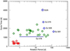 |
Fig. 1. Cycle times vs. rotation period (both in days) for early M stars (rhombic symbols). Among the group of rapid rotators with rotation periods less than a day (Vida et al. 2014) are also the early M dwarfs EY Dra and V405 And (Vida et al. 2013). The remaining data are from Suárez Mascareño et al. (2016); Wargelin et al. (2017), and Distefano et al. (2017). For GJ476 the cycle time is known but not the rotation period (blue bar). The Schwabe cycle of the Sun is indicated as an asterisk denoted SUN. |
Gomes da Silva et al. (2012) give further examples of M dwarfs with cycle lengths between three and five years. It is of particular importance to know the relation of the cycle time with the rotation time for a homogeneous sample of stars. Savanov (2012) used light curves of cool M dwarfs to find long-term cycle variations up to timescales of years. His sample is mixed by M stars with outer convection zones and also fully convective stars. There seems to be no systematic dependence of the cycle time on the rotation time even for subsamples with slow and fast rotations.
An independent study about the coupling of rotation and cycle times for fast-rotating cool stars has been published by Vida et al. (2014). Among the analyzed 39 Kepler light curves of late-type stars with rotation periods shorter than one day, nine examples showed cyclic variations with periods between one and three years. Moreover, from variations of the rotation periods, lower limits of the latitudinal differential rotation were derived with characteristic differences δΩ ≲ 0.03 rad d−1. Three of these targets (KIC04953358, KIC05791720, KIC10515986) have effective temperatures below 4000 K and can be considered early M dwarfs. Their minimum latitudinal shear δΩ reaches from 0.008 rad d−1 to 0.03 rad d−1, which are values close to the theoretical results for ZAMS stars with M = 0.5 M⊙ by Küker & Rüdiger (2011). The related meridional surface flow for fast rotation reaches amplitudes of 10 m s−1.
In this paper, we collected currently available data on cycle periods of M dwarfs from the literature and compare these with our numerical predictions. In Sect. 2, we reanalyze part of the All Sky Automated Survey (ASAS; Pojmanski 1997) database for cycle periods, and present new STELLA photometry for three M dwarfs (GJ270, GJ328, GJ476) that had hitherto unknown rotational periods. In Sect. 3, we discuss the basic mechanisms of advection-dominated dynamos and present in Sect. 4 new models for the large-scale flows in the outer convection zone of early M stars. Section 5 summarizes our conclusions. The resulting surface values of the equator-to-pole differences of the angular velocity fit the observational data while the meridional flow amplitudes are basically too low to be responsible for the observed M-star cycle periods.
2. Observational data
2.1. Cycle periods
From the literature we adopt only cycles from long-term changes of photometric time-series data with two constrains. Firstly, cycle periods are only accepted if the photometry was well sampled, that is only if there is no years-long interruption in the measurements that could introduce aliasing periods. Secondly, we require that the cycle period is not near the length of the data set itself, that is only if the changes were repeated or nearly repeated. A total of 25 targets were selected. For an earlier version of this approach, we refer to Oláh & Strassmeier (2002). All rotational and cycle periods used in this paper are listed in Table 1.
Rotation periods, differential rotation, and cycle times of early M dwarfs used in the present paper.
We re-examined the ASAS observations (Kiraga & Stepien 2007) analyzed by Savanov (2012) where many cycles were given for each star but the values themselves not published. We applied a time-frequency analysis on the same data sets with a bilinear time-frequency transformation method such as that used by Oláh et al. (2009). For a description of this approach we refer to Kolláth & Oláh (2009). Out of the available 31 targets, cycles for 19 targets could be verified and added to our sample. The results are given in Table 1 for stars of spectral type M3.5 or earlier. In most cases only a single cycle is found. For GJ729 and GJ897 two cycles were found but are harmonics where we cannot decide which one is correct, while in case of GJ182, GJ2036A, GJ3367 and GJ803 the two detected cycle periods seem unrelated. The very fast-rotating star GJ890 (=HK Aqr) exhibits a single 3–4 yr cycle. Generally, the ASAS data do not allow constraining cycles of around one year due to the relatively low precision and low time resolution because the survey was designed for other purposes. The case for the fast-rotating Kepler stars is similar, but then because of limited overall time coverage.
Since multiple cycles similar to the known solar cycles are also observed on stars (Oláh et al. 2009, 2016), it is important to identify those stellar cycles that are true analogs of the dominating solar dynamo (Schwabe) cycle. The Sun seems to exhibit at least three cycle periods (but see Beer et al. 2018 for a full discussion): a mid-term cycle with 3–4 yr, the Schwabe cycle with 9–14 yr, and the Gleissberg cycle with 90 yr or more. The Schwabe cycle is, by far, the dominating cycle and can be traced from the solar butterfly diagram showing the latitude migration of the sunspots in the course of a cycle. This is not directly doable for stars yet, but see the review by Strassmeier (2005) for a summary of stellar cycle observations and tracers.
We note the many attempts of measuring stellar cycles from photometric time series. In Vida et al. (2014) quasi-periodic changes of the rotational periods have been derived from the extremely precise Kepler data sets, based on the unresolved pattern of a solar-like butterfly diagram. Such changes on a number of fast-rotating (Prot < 1 day) M dwarfs were found, which reflect the appearance of the spot’s latitudes throughout an activity cycle. Therefore, we assume that the comparably short variability changes of the fast-rotating M dwarfs (Prot < 1 day) in the sample of Vida et al. (2014) are most probably the true dynamo cycles of the stars.
Evidence of multiple cycles in fast-rotating M dwarfs are found for two well-observed stars from high precision ground-based data. V405 And and EY Dra show cycle periods of less than a year (Vida et al. 2013), similar to the stars of the Kepler field (Vida et al. 2014). However, the corresponding Fig. 1 from Vida et al. (2014) clearly shows, that these stars have additional, longer cyclic changes on timescales of roughly 4–5 years or even longer. The shorter cycles (< 1 year) of V405 And and EY Dra are then likely the basic dynamo cycles similar to those of the Kepler stars. An example of a more massive star than an early M dwarf, but significantly lower mass than the Sun, is LQ Hya (K2V). This star has a rotational period of 1.6 days, whereas the Sun (G2V) has 27.24 days. The shorter cycle of LQ Hya is about three years and corresponds to the solar 11 yr cycle given its dominance, the longer cycle of 7–12 yr may be an analog of the solar Gleissberg cycle (Oláh & Strassmeier 2002).
2.2. Rotation periods
The new rotation periods in this paper also come from photometry. In particular, the rotation periods for the Gliese-Jahreiss (GJ) stars observed by ASAS are from the same data set as used for the cycle times, from simple Fourier analysis. The other periods are from the literature and referred to in Table 1.
Three GJ stars have a cycle period from the literature but not a rotation period (Robertson et al. 2013a). Therefore, these three stars (GJ270, GJ328, and GJ476) were put on the observing menu of one of our robotic STELLA telescopes in Tenerife for photometric monitoring. GJ270 and GJ328 were observed for a duration of four months, GJ476 was observed for 40 nights, and all of these stars were observed in 2017–18. The STELLA-I telescope and its wide-field imaging photometer WiFSIP were employed. The WiFSIP instrument provides a field of view of 22′ × 22′ on a scale of 0.32″ pixel−1. The detector is a 4096 × 4096 CCD with 15 μm pixels−1. The observations were performed in blocks of five exposures in Johnson V (150 s exposure time) and five exposures in Cousins I (60 s). Data reduction and aperture photometry was done with the same ESO-MIDAS routines already used for similar monitoring programs of exoplanet host stars (Mallonn et al. 2015, 2018). The light curves versus Julian date are shown in Appendix A.
We applied the minimum string-length method described in Dworetsky (1983) as well as a Lomb-Scargle periodogram to all three data sets (for two bandpasses each). None of the three targets exhibit variability significantly above the 1% level in either bandpass which makes our periods tentative. GJ270 seems to be the best detection with a period of ≈30 d and an amplitude of 10 mmag with a false alarm probability (fap) of 0.18%. The Lomb-Scargle method gave additionally a period of 8.7 d which, however, is not seen from the minimum string length method and thus is rejected. A similar period of 33.6 d is obtained for GJ328 with a fap of 0.3% and same amplitude. The Lomb-Scargle periodogram remained inconclusive for this target. The third star, GJ476, has no detection. Its largest minimizations are achieved with a very large fap of ≈7% at periods of 11 d and 1.1 d but, more likely, the true period is longer than the 40 nights of observation. Again, its Lomb-Scargle periodogram did not show a significant peak.
3. Advection-dominated dynamos
Meridional circulations influence the mean-field dynamo. This influence can be only a small modification if its characteristic timescale τm basically exceeds the cycle time τcyc. In this case, um represents the latitudinal flow close to the base of the convection zone. Positive um denotes a flow toward the equator. The cycle period becomes shorter for clockwise flow (in the first quadrant) but it becomes longer for counterclockwise flow (Roberts & Stix 1972), which is observed on the Sun. For a critical meridional circulations, when τm ≲ τcyc, the αΩ dynamo stops operation (in particular if the dynamo wave and flux transport act in opposite directions).
For the solar cycle and with the estimate τm ≃ R/um, we find um ≃ 2 m s−1 as a critical value above which the dynamo process is dominated by the flow and where in many models the cycle time varies as 1/um (Dikpati & Charbonneau 1999; Küker et al. 2001; Bonanno et al. 2002). Short cycles need fast flow to be the result of an advection-dominated dynamo. Plausibly, the speed of the meridional circulation in convection zones grows with the rotation rate. Cycle time and rotation time are thus positively correlated in the mentioned dynamo models. The data for our early M stars collected in Table 1 and plotted in Fig. 1 do not contradict this condition. However, because standard αΩ dynamos can also show a (light) positive correlation of cycle time and rotation time (Rüdiger et al. 1994), the shape of the function Ωcyc(Ω) may not help to find the nature of the operating dynamo.
A critical magnetic Reynolds number for advection-dominated dynamos is given by
 (2)
(2)
so that um = 10 m s−1 is the minimal flow speed for ηT = 1012 cm2 s−1 and D ≈ 100 000 km. It is the main question of this paper whether for the above-mentioned fast-rotating M stars the conditions for the operation of a flux-dominated dynamo are fulfilled. If we know the cycle times from observations it is only necessary to know the meridional flow amplitudes for the given rotation rates. An advection-dominated dynamo can only operate if the cycles are longer than the turnover times of the meridional flow. The ratio
 (3)
(3)
exceeds unity for advection dominated dynamos if the travel time τm is estimated by τm ≃ πRb/um with Rb the radius of the bottom of the convection zone. We find τ ≃ 4 for all models of Dikpati & Charbonneau (1999), Küker et al. (2001), and Bonanno et al. (2002).
For τ < 1 the operation of such a dynamo mechanism can be excluded. It is now possible to calculate by means of the theory of differential rotation (see next section) the amplitudes of the meridional flow at the bottom of the convection zone. In particular the fast-rotating Kepler stars in Fig. 1 are interesting candidates for high enough flow speeds of the meridional circulation. The travel time τm at the bottom of the convection zone can be estimated with πRbot/um with Rbot as the radius of the base of the convection zone. For M stars the travel time varies from 13 years for um ≃ 1 m s−1 to 1.3 years for um = 10 m s−1. Therefore, a rather precise theory of the meridional flow is needed to calculate the true amplitude of um.
4. Differential rotation and meridional flow
The theory of differential rotation in stellar convection zones provides simultaneous results for the rotation law and meridional flow if the rotation rate is known (Rüdiger et al. 2013). For the M dwarfs collected in Fig. 1 the rotation rates are indeed known. Using spherical polar coordinates, it is possible to reduce the Reynolds equation to a system of two partial differential equations. The azimuthal component of the Reynolds equation expresses the conservation of angular momentum,
 (4)
(4)
where t is the angular momentum flux vector with the components
 (5)
(5)
with the angular velocity Ω, the meridional flow velocity um, and the azimuthal components of the Reynolds stress, Qϕi.
The equation for the meridional flow is derived from the Reynolds equation by taking the azimuthal component of its curl,
![Mathematical equation: $$ \begin{aligned} \left[\nabla \times \frac{1}{\rho }\nabla \cdot R \right]_\phi + r \sin \theta \frac{\partial \Omega ^2}{\partial z} + \frac{1}{\rho ^2}(\nabla \rho \times \nabla p)_\phi + \cdots = 0, \end{aligned} $$](/articles/aa/full_html/2019/02/aa33173-18/aa33173-18-eq7.gif) (6)
(6)
where Rij = −ρQij is the Reynolds stress and ∂/∂z is the derivative along the axis of rotation. The Λ effect appears in two components of the Reynolds stress,
 (7)
(7)
In this equation,  and
and  contain only first order derivatives of Ω with respect to r and θ and therefore vanish for uniform rotation. The coefficients V and H refer to the vertical and horizontal part of the Λ effect. The function V is negative for slow rotation and becomes very small for fast rotation while H is positive-definite and almost vanishes for slow rotation. Its existence seems to have been proven at the solar surface by Solar Dynamics Observatory HMI data (Rüdiger et al. 2014). The Coriolis number Ω* = 2τcorrΩ exceeds unity almost everywhere in the convection zone except in the outer layers. Close to Ω* = 1 this number is V ≃ H so that at the equator the radial angular momentum flux vanishes. The negativity of V for slow rotation provides the negative shear in the solar super-granulation layer and it also allows anti-solar rotation for Ω* < 1.
The equations for the large-scale flows in convection zones have been solved for the Sun and for cool main-sequence stars (Küker et al. 2011; Küker & Rüdiger 2011) where the results for the pole-to-equator differences of Ω and the surface values of the (poleward) meridional flow agree well with the observational data. At the bottom of the solar convection zone the resulting flow amplitude is about 6 m s−1. The travel time of a gas parcel from pole to equator is thus about 6.5 years, shorter than the cycle time of 11 yr. An advection-dominated dynamo for the Sun is thus possible but only if after (2) the Eddy diffusivity does not exceed 6 × 1011 cm2 s−1, which is not easy to explain.
For the meridional flows in M dwarfs the theoretical results are summarized in the Figs. 2 and 3. Figure 2 shows isocontours of the stream function ψ defined through
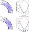 |
Fig. 2. Meridional flow system for two models for a star with a mass of M = 0.60 M⊙ and a rotation period of 1 day (top panels) and 10 days (bottom panels). Left panel: isocontours of the stream function. We find poleward circulation at the top of the convection zone (blue full line) and equatorward flow at the base of the convection zone (red dashed line). |
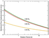 |
Fig. 3. Meridional flow amplitudes um averaged over the latitude at the bottom of the convection zones in m s−1 for the three different stellar models with masses of M = 0.40 M⊙ (yellow), M = 0.60 M⊙ (red), and M = 0.66 M⊙ (green). This refers to the rotation-law results in Fig. 5. |
 (8)
(8)
for rotation periods of one day (top panel) and ten days (bottom panel) as well as the flow speeds at the top and bottom of the convection zone. There is always one cell per hemisphere with the surface flow directed toward the poles and the return flow at the bottom of the convection zone. The amplitude of the return flow is between 4 m s−1 for slow rotation and 7 m s−1 for fast rotation. The flow patterns from our differential rotation model show a rather strong concentration of the flow at the top and bottom boundaries. This does, however, not prevent the flux transport dynamo, as has been shown by its successful use in modeling the magnetic field of AF Lep in Järvinen et al. (2015).
Figure 3 plots the circulation velocities at the bottom of the convection zones averaged over latitude for three solar metallicity ZAMS models, which were computed with the MESA stellar evolution code (Paxton et al. 2011). The masses were chosen to cover the spectral types of the stars in Table 1. The meridional flows are fastest for rapid rotation and they grow with growing effective temperature. Above 4000 K, however, the amplitudes um seem to saturate while for the M dwarfs below this temperature the um become basically smaller. For a rotation period of about one day a flow with um ≃ 3.5 m s−1 is obtained. Therefore, for such rapidly rotating M dwarfs the travel time is 3.5 years or 1360 d, which is much longer than the observed cycle periods of about 1 year. At least, for the fast-rotating Kepler stars given by Vida et al. (2014) the dynamo process cannot be of the advection-dominated type.
Figure 4 demonstrates that for all rotators the calculated travel times exceed the observed cycle times. The cycles are too short to be originated by the meridional circulation. The circulation is thus only able to produce slight modifications in dependence on the rotation rate. Therefore, the existence of an advection-dominated dynamo is not confirmed by Fig. 4 for the sample of fast-rotating late-type stars.
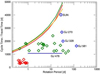 |
Fig. 4. Calculated travel times (in days, colored lines) and the observed cycle times for the early M stars from Fig. 1 as a function of rotation period. The cycle times are always shorter than the calculated travel times, i.e., always τ ≲ 1. The data for the Sun are shown for comparison. Colors as in Fig. 3. For GJ476 (blue bar) the cycle period is known but not the rotation period. |
As the stellar radii are smaller for cooler stars, the travel times for our three stellar models are almost identical (Fig. 4). The travel times strongly increase with slower rotation, that is increase with rotation period. For all stars with masses 0.40–0.66 M⊙ and with, say, solar rotation rate, the cycle time will be close to 11 yr. None of the observed cycle times for early M stars lies above the single mixed-colored line, none of the observed cycle times exceeds the travel times from pole to equator for the early M stars so that the main condition for the existence of advection-dominated dynamos is nowhere fulfilled.
The evaluation of the meridional flow dynamics is only one side of the medal. The equation system simultaneously provides the rotation law of the convection zones. We can only be relatively sure about the results for the meridional circulation inside the convection zone in case the theoretically resulting equator-to-pole differences of the stellar rotation rate also comply with the observations. Figure 5 shows the influences of the stellar structure and rotation rate on the equator-to-pole difference of the angular velocity. The calculations are validated for ZAMS models with masses of 0.66 M⊙, 0.60 M⊙, and 0.40 M⊙. For Z = 0.02 the models cover a temperature interval between 4325 K and 3581 K. The late K or early M stars are best described by M = 0.60 M⊙ and Teff = 4038 K.
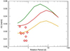 |
Fig. 5. Comparison of the shear values δΩ from Vida et al. (2014) for fast-rotating M stars with our calculated values. The calculated values are shown as lines for stars of M = 0.66 M⊙ (green, top line), M = 0.60 M⊙ (red, middle line), and M = 0.40 M⊙ (yellow, bottom line). |
For all stellar models the equator-to-pole differences of the surface rotation law grow with the rotation period if the rotation is not too slow. The theoretical shear grows for rotation periods of one day to ten days approximately by 50%. For even slower rotation the rotational quenching of the Λ effect leads to a reduction of the shear. The maximum of values of the differential rotation δΩ appears for rotation periods slightly shorter than ten days. For slower rotation the shear slowly decays by the rotational quenching of the Λ effect. We note that there are even strong differences of the resulting δΩ for the two models with similar masses that, however, disappear for very fast and very slow rotation.
We find that the red line in Fig. 5 for a temperature of Teff = 4038 K describes the behavior of the early M stars best. The minimal value of the equator-to-pole difference is δΩ ≃ 0.028 for stars rotating slightly faster than one day. The result nearly perfectly fits the observations, which on average yield minimal values. The mean-field model of the hydrodynamic flows in the convection zone thus provides a correct interpretation of the differential rotation data, which may support the reliability of the results for the meridional circulation at the bottom of the convection zones.
5. Conclusions
We have shown that the observed activity cycles of the early-type M dwarfs are so short that they cannot be understood by an advection-dominated dynamo model. There is no single observation where the cycle period remarkably exceeds the computed travel time from pole to equator. The hydrodynamical model on basis of the Λ effect, which exists in rotating convection zones (see Rüdiger et al. 2014), provides a combination of differential rotation and meridional flow for a given stellar model. The computed differential rotation at the stellar surface complies with the observations for fast-rotating Kepler stars of spectral classes early M. It is thus allowed to use the meridional flow amplitudes, which are simultaneously provided by the model, as the characteristic amplitude for the flow pattern. As shown in Fig. 4 the travel times strongly depend on the stellar rotation period which, however, is not so obvious for the cycle times. The early M stars do not fulfill the main condition of the advection dynamo concept that requires that the ratio in Eq. (3) exceeds unity.
Acknowledgments
K.O. thanks for the support from the MTA CSFK Discretional Fund.
References
- Beer, J., Tobias, S. M., & Weiss, N. O. 2018, MNRAS, 473, 1596 [NASA ADS] [CrossRef] [Google Scholar]
- Bonanno, A., Elstner, D., Rüdiger, G., & Belvedere, G. 2002, A&A, 390, 673 [NASA ADS] [CrossRef] [EDP Sciences] [Google Scholar]
- Dikpati, M., & Charbonneau, P. 1999, ApJ, 518, 508 [NASA ADS] [CrossRef] [Google Scholar]
- Distefano, E., Lanzafame, A. C., Lanza, A. F., Messina, S., & Spada, F. 2016, A&A, 591, A43 [NASA ADS] [CrossRef] [EDP Sciences] [Google Scholar]
- Distefano, E., Lanzafame, A. C., Lanza, A. F., Messina, S., & Spada, F. 2017, A&A, 606, A58 [NASA ADS] [CrossRef] [EDP Sciences] [Google Scholar]
- Dworetsky, M. M. 1983, MNRAS, 203, 917 [NASA ADS] [Google Scholar]
- Gomes da Silva, J., Santos, N. C., Bonfils, X., et al. 2012, A&A, 541, A9 [NASA ADS] [CrossRef] [EDP Sciences] [Google Scholar]
- Järvinen, S. P., Arlt, R., Hackman, T., et al. 2015, A&A, 574, A25 [NASA ADS] [CrossRef] [EDP Sciences] [Google Scholar]
- Johnson, M. C., Endl, M., Cochran, W. D., et al. 2016, ApJ, 821, 74 [NASA ADS] [CrossRef] [Google Scholar]
- Kiraga, M., & Stepien, K. 2007, Acta Astron., 57, 149 [NASA ADS] [Google Scholar]
- Köhler, H. 1973, A&A, 25, 467 [NASA ADS] [Google Scholar]
- Kolláth, Z., & Oláh, K. 2009, A&A, 501, 695 [NASA ADS] [CrossRef] [EDP Sciences] [Google Scholar]
- Küker, M., & Rüdiger, G. 2011, Astron. Nachr., 332, 933 [NASA ADS] [CrossRef] [Google Scholar]
- Küker, M., Rüdiger, G., & Schultz, M. 2001, A&A, 374, 301 [NASA ADS] [CrossRef] [EDP Sciences] [Google Scholar]
- Küker, M., Rüdiger, G., & Kitchatinov, L. L. 2011, A&A, 530, A48 [NASA ADS] [CrossRef] [EDP Sciences] [Google Scholar]
- Künstler, A., Carroll, T. A., & Strassmeier, K. G. 2015, A&A, 578, A101 [NASA ADS] [CrossRef] [EDP Sciences] [Google Scholar]
- Mallonn, M., Nascimbeni, V., Weingrill, J., et al. 2015, A&A, 583, A138 [NASA ADS] [CrossRef] [EDP Sciences] [Google Scholar]
- Mallonn, M., Herrero, E., Juvan, I. G., et al. 2018, A&A, 614, A35 [NASA ADS] [CrossRef] [EDP Sciences] [Google Scholar]
- Noyes, R. W., Weiss, N. O., & Vaughan, A. H. 1984, ApJ, 287, 769 [NASA ADS] [CrossRef] [Google Scholar]
- Oláh, K., & Strassmeier, K. G. 2002, Astron. Nachr., 323, 361 [NASA ADS] [CrossRef] [Google Scholar]
- Oláh, K., Kolláth, Z., Granzer, T., et al. 2009, A&A, 501, 703 [NASA ADS] [CrossRef] [EDP Sciences] [Google Scholar]
- Oláh, K., Kővári, Z., Petrovay, K., et al. 2016, A&A, 590, A133 [NASA ADS] [CrossRef] [EDP Sciences] [Google Scholar]
- Paxton, B., Bildsten, L., Dotter, A., et al. 2011, ApJS, 192, 3 [Google Scholar]
- Pojmanski, G. 1997, Acta Astron., 47, 467 [NASA ADS] [Google Scholar]
- Roberts, P. H. 1972, Philos. Trans. R. Soc. London Ser. A, 272, 663 [NASA ADS] [CrossRef] [Google Scholar]
- Roberts, P. H., & Stix, M. 1972, A&A, 18, 453 [NASA ADS] [Google Scholar]
- Robertson, P., Endl, M., Cochran, W. D., & Dodson-Robinson, S. E. 2013a, ApJ, 764, 3 [NASA ADS] [CrossRef] [Google Scholar]
- Robertson, P., Endl, M., Cochran, W. D., MacQueen, P. J., & Boss, A. P. 2013b, ApJ, 774, 147 [NASA ADS] [CrossRef] [Google Scholar]
- Robertson, P., Mahadevan, S., Endl, M., & Roy, A. 2014, Science, 345, 440 [NASA ADS] [CrossRef] [Google Scholar]
- Rüdiger, G., Kitchatinov, L. L., Küker, M., & Schultz, M. 1994, Geophys. Astrophys. Fluid Dyn., 78, 247 [NASA ADS] [CrossRef] [Google Scholar]
- Rüdiger, G., Küker, M., & Schnerr, R. S. 2012, A&A, 546, A23 [NASA ADS] [CrossRef] [EDP Sciences] [Google Scholar]
- Rüdiger, G., Kitchatinov, L. L., & Hollerbach, R. 2013, Magnetic Processes in Astrophysics: Theory, Simulations, Experiments (Weinheim: Wiley-VCH) [CrossRef] [Google Scholar]
- Rüdiger, G., Küker, M., & Tereshin, I. 2014, A&A, 572, L7 [NASA ADS] [CrossRef] [EDP Sciences] [Google Scholar]
- Savanov, I. S. 2012, Astron. Rep., 56, 716 [NASA ADS] [CrossRef] [Google Scholar]
- Schmitt, D., & Schuessler, M. 1989, A&A, 223, 343 [NASA ADS] [Google Scholar]
- Schrijver, C. J., & Martin, S. F. 1990, Sol. Phys., 129, 95 [NASA ADS] [CrossRef] [Google Scholar]
- Spada, F., Demarque, P., Kim, Y.-C., Boyajian, T. S., & Brewer, J. M. 2017, ApJ, 838, 161 [Google Scholar]
- Strassmeier, K. G. 2005, Astron. Nachr., 326, 269 [NASA ADS] [CrossRef] [Google Scholar]
- Suárez Mascareño, A., Rebolo, R., & González Hernández, J. I. 2016, A&A, 595, A12 [NASA ADS] [CrossRef] [EDP Sciences] [Google Scholar]
- Vida, K., Kriskovics, L., & Oláh, K. 2013, Astron. Nachr., 334, 972 [Google Scholar]
- Vida, K., Oláh, K., & Szabó, R. 2014, MNRAS, 441, 2744 [NASA ADS] [CrossRef] [Google Scholar]
- Wargelin, B. J., Saar, S. H., Pojmański, G., Drake, J. J., & Kashyap, V. L. 2017, MNRAS, 464, 3281 [NASA ADS] [CrossRef] [Google Scholar]
Appendix A: STELLA photometry of GJ270, GJ328, and GJ476
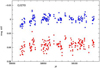 |
Fig. A.1. Light curve of GJ270. Time is in Julian dates plus 2 400 000. Shown is the differential magnitudes for the V band (blue dots, upper band) and the IC bad (red dots, lower band). |
All Tables
Rotation periods, differential rotation, and cycle times of early M dwarfs used in the present paper.
All Figures
|
Fig. 1. Cycle times vs. rotation period (both in days) for early M stars (rhombic symbols). Among the group of rapid rotators with rotation periods less than a day (Vida et al. 2014) are also the early M dwarfs EY Dra and V405 And (Vida et al. 2013). The remaining data are from Suárez Mascareño et al. (2016); Wargelin et al. (2017), and Distefano et al. (2017). For GJ476 the cycle time is known but not the rotation period (blue bar). The Schwabe cycle of the Sun is indicated as an asterisk denoted SUN. |
| In the text | |
|
Fig. 2. Meridional flow system for two models for a star with a mass of M = 0.60 M⊙ and a rotation period of 1 day (top panels) and 10 days (bottom panels). Left panel: isocontours of the stream function. We find poleward circulation at the top of the convection zone (blue full line) and equatorward flow at the base of the convection zone (red dashed line). |
| In the text | |
|
Fig. 3. Meridional flow amplitudes um averaged over the latitude at the bottom of the convection zones in m s−1 for the three different stellar models with masses of M = 0.40 M⊙ (yellow), M = 0.60 M⊙ (red), and M = 0.66 M⊙ (green). This refers to the rotation-law results in Fig. 5. |
| In the text | |
|
Fig. 4. Calculated travel times (in days, colored lines) and the observed cycle times for the early M stars from Fig. 1 as a function of rotation period. The cycle times are always shorter than the calculated travel times, i.e., always τ ≲ 1. The data for the Sun are shown for comparison. Colors as in Fig. 3. For GJ476 (blue bar) the cycle period is known but not the rotation period. |
| In the text | |
|
Fig. 5. Comparison of the shear values δΩ from Vida et al. (2014) for fast-rotating M stars with our calculated values. The calculated values are shown as lines for stars of M = 0.66 M⊙ (green, top line), M = 0.60 M⊙ (red, middle line), and M = 0.40 M⊙ (yellow, bottom line). |
| In the text | |
|
Fig. A.1. Light curve of GJ270. Time is in Julian dates plus 2 400 000. Shown is the differential magnitudes for the V band (blue dots, upper band) and the IC bad (red dots, lower band). |
| In the text | |
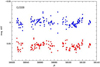 |
Fig. A.2. Light curve of GJ328. Otherwise as in Fig. A.1. |
| In the text | |
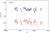 |
Fig. A.3. Light curve of GJ476. Otherwise as in Fig. A.1. |
| In the text | |
Current usage metrics show cumulative count of Article Views (full-text article views including HTML views, PDF and ePub downloads, according to the available data) and Abstracts Views on Vision4Press platform.
Data correspond to usage on the plateform after 2015. The current usage metrics is available 48-96 hours after online publication and is updated daily on week days.
Initial download of the metrics may take a while.