| Issue |
A&A
Volume 621, January 2019
|
|
|---|---|---|
| Article Number | A136 | |
| Number of page(s) | 7 | |
| Section | Stellar structure and evolution | |
| DOI | https://doi.org/10.1051/0004-6361/201834319 | |
| Published online | 18 January 2019 | |
Discovery of short-term activity cycles in F-type stars
1
Hamburger Sternwarte, Universität Hamburg, Gojenbergsweg 112, 21029 Hamburg, Germany
e-mail: mmittag@hs.uni-hamburg.de
2
Department of Astronomy, University of Guanajuato, Mexico
Received:
25
September
2018
Accepted:
16
November
2018
Previous studies have revealed a 120 day activity cycle in the F-type star τ Boo, which represents the shortest activity cycle discovered until now. The question arises as to whether or not short-term activity cycles are a common phenomenon in F-type stars. To address this question, we analyse S-index time series of F-type stars taken with the TIGRE telescope to search for periodic variations with a maximal length of 2 years using the generalised Lomb-Scargle periodogram method. In our sample, we find four F-type stars showing periodic variations shorter than one year. However, the amplitude of these variations in our sample of F-star type stars appears to be smaller than that of solar-type stars with well-developed cyclic activity, and apparently represents only a part of the total activity. We conclude that among F-stars, the time-behaviour of activity differs from that of the Sun and cooler main sequence stars, as short-term cyclic variations with shallow amplitude of the cycle seem to prevail, rather than cycles with 10+ years periods and a larger cycle amplitude.
Key words: stars: activity / stars: atmospheres / stars: chromospheres / stars: late-type
© ESO 2019
1. Introduction
While the 11-year activity cycle of our Sun was already discovered by Schwabe (1844), the systematic search for activity cycles in main sequence stars only started with the Mount Wilson HK program (Wilson 1978; Baliunas et al. 1995), which began in 1966 and terminated at the end of the last century. In a landmark paper Baliunas et al. (1995) presented the time series of 112 stars from the Mount Wilson HK program, including the Sun observed as a star, and found activity cycles in 46 stars. Depending on the false alarm probability (FAP), Baliunas et al. (1995) assigned a grade to each of the determined cycles and labelled the cycles as “excellent” (FAP ≤10−9), “good” (10−9< FAP ≤10−5), “fair” (10−5< FAP ≤ 10−2), and “poor” (10−2< FAP ≤10−1).
In nine stars, Baliunas et al. (1995) also found a secondary cycle, while the shortest reported activity cycle (for the G-type star HD 76151) has a period of 2.52 yr with a FAP grade “fair”. Ten of the 46 stars with a determined activity cycle are F-type stars with cycles being assigned only the FAP grade “fair” or “poor”. The shortest cycle among the investigated F-type stars is 3.56 yr with the FAP grade “fair” for the star HD 100180. The remaining stars without any significant period were categorised by Baliunas et al. (1995) into four classes, namely “flat”, “flat?”, “long” or “var” depending on the ratio of the scatter and mean S-value. Those stars categorised as “flat” have σS/S < 1%−1.5%, “flat?” have σS/S ≈ 1.5%−2.%, “var” have σS/S > 2% without a significant periodic signal in the time range from 1 to 25 years, and “long” refers to stars with variability on a timescale longer than 25 years.
As far as solar-type, pronounced (“excellent” or “good” in the nomenclature of Baliunas et al. 1995) cycles of a period of approximately 10 yr or more are concerned, by placing the Mount Wilson sample stars in the HR diagram, Schröder et al. (2013) found that the Sun seems to be near the upper end of such detections on the main sequence, while most other pronounced cycles are found among somewhat cooler, less massive stars (see Fig. 4 in that paper). Consequently, F-stars do not show the same form of solar-type activity with long, pronounced cycles. What therefore is their activity like in the time-domain?
In the bright F-type star τ Boo (HD 120136), Baliunas et al. (1995) report an activity cycle with a length of 11.6 yr; however, with the FAP grade “poor”. Baliunas et al. (1997) also mention a 116 day “variation” in their Ca II data for τ Boo without providing any details for the estimation and nature of this variation. In new and independent S-index data, Mengel et al. (2016) and Mittag et al. (2017) found an activity cycle ≈117 days and ≈122 days, respectively. Simultaneously, Schmitt & Mittag (2017) re-analysed the Mount Wilson S-index time series of τ Boo in detail and confirmed the presence of such a short-period cycle over the past 40 years. Mittag et al. (2017) also showed that X-ray data support a periodicity of about 120 days. As far as short-term activity cycles in F-type stars are concerned, we note that Metcalfe et al. (2010) found a 1.6 yr activity cycle for ι Hor (HD 17051; spectral type F8) and García et al. (2010) report an indication for at least a 120 day cycle for HD 49933 (spectral type F3). Thus the question arises as to how common short-term cycles in F-type stars are.
Our long-term monitoring program of stellar activity performed with the TIGRE telescope (Schmitt et al. 2014) also contains F-type stars, which we examined for the presence of short-term activity cycles. Higher cadence thanks to the robotic operation of TIGRE and precise S-measurements thanks to a high signal-to-noise ratio (S/N) in line cores of the Ca II H&K lines – for example for HD 16673 a mean S/N of 100 in the 1 Å band pass – make these observational data especially suitable for this task. Here we present the results for four F-stars, namely HD 16673, HD 49933, HD 75332, and HD 100563, which show clear evidence for short-term cycles in their activity-related chromospheric emission.
2. Observations
Table 1 provides some details on the three stars discussed in this paper, that is, visual magnitude V and B − V colour (taken from HIPPARCOS catalogue ESA 1997) together with the total number of TIGRE S-index measurements available. The TIGRE telescope is a fully robotic telescope with a 1.2 m aperture, located at the La Luz Observatory near Guanajuato, Mexico. Its only instrument is the two-channel fibre-fed Échelle spectrograph HEROS with a wavelength range from 3800 Å to 8800 Å with a 100 Å gap at 5800 Å and a spectral resolution of R ≈ 20 000; a detailed description of the TIGRE facility is given by Schmitt et al. (2014).
Object and observational information.
The spectral data are reduced with the TIGRE/HEROS standard reduction pipeline version v3.1, implemented in IDL and based on the IDL reduction package REDUCE (Piskunov & Valenti 2002). The TIGRE/HEROS pipeline is designed as a fully automatic data-reduction pipeline and includes all necessary reduction steps for Échelle spectra; a detailed description of an older TIGRE/HEROS pipeline version is given by Mittag et al. (2010) and additional general information on the pipeline is provided by Hempelmann et al. (2016) and Mittag et al. (2016).
An additional feature implemented in the TIGRE/HEROS reduction pipeline is the automatic estimation of the instrumental S-index (STIGRE), defined as (Mittag et al. 2016)
where NH and NK are the Ca II H&K line intensities summed in a 1 Å wide rectangular band pass centred on the H and K lines, respectively, and NR and NV are the summed intensities in two 20 Å-wide band passes centred on 3901.07 Å and 4001.07 Å, respectively. The instrumental STIGRE index can be converted with a linear relation into the so-called Mount Wilson S-index (SMWO), the classical and commonly used activity index, through the equation

Further general information on the automatic estimation of STIGRE and the derivation of Eq. (2) can be found in Mittag et al. (2016).
The S-index transformation given in Eq. (2) was derived with STIGRE data taken until May 2015 and from spectra reduced with the data-reduction pipeline version 1. In the meantime, the pipeline has been updated and more S-values have been obtained for our calibration stars [see Table 2 of ][]Mittag2016. Therefore, we decided to check our S-index calibration, but found no significant changes. Next, we tested the influence of different versions of the data-reduction pipeline on our S-index values: We first compared the mean TIGRE S-data computed with the different reduction versions and found a mean scatter between the mean S-data of less than 1%. In Fig. 1 we show the ratio of mean TIGRE Mount Wilson S-index of our calibration stars obtained using different pipeline versions versus the TIGRE Mount Wilson S-index from the last pipeline version. The upgrade of the data-reduction pipeline has a larger influence on the individual S-index than on the mean S-index, meaning that the individual S-index values can show more variation. An important upgrade of the pipeline was the improvement of the treatment of cosmics which can impact the S-index calculation. To quantify this dispersion, we computed the difference between the S-values obtained from the different reductions and determined the scatter. We find a mean scatter of 1.5% in the difference between the S-data computed with the different reduction version and conclude that the different reduction versions have no significant influence on the mean S-value, except for the individual S-values at a level of 1.5% on the mean.
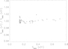 |
Fig. 1. Ratio of the mean TIGRE S-data obtained from the reduction pipelines. |
3. Data analysis
3.1. Period, error of the period, and false-alarm probability estimation
To search for periodic variations in our S-index time series, we use the generalised Lomb-Scargle (GLS) method by Zechmeister & Kürster (2009). For this analysis, we used our own Python code based on the equations presented by Zechmeister & Kürster (2009). The GLS formalism assumes a sinusoidal wave form with a constant offset and calculates a χ2-value using the model ansatz

where A, B, and C are constants calculated from the data yi with uncertainty σi at the times ti, i =...N, where N denotes the number of data points. The GLS periodogram is calculated with the expression (Zechmeister & Kürster 2009)
where  is the χ2-value from the weighted mean and is used for the normalisation of χ2(ω); a detailed description and derivation of the GLS method is given by Zechmeister & Kürster (2009).
The error in the determined period is estimated using the equation (Baliunas et al. 1995)
where σn denotes the standard deviation of the residuals (O–C), P the period, T the total length of the observation interval, A the amplitude of the signal, and N the total number of data points.
For the FAP estimation, we use the method described by Zechmeister & Kürster (2009), who define the FAP as
![$$ \begin{aligned} \mathrm{FAP} = 1-[1-\mathrm{Prob}(p>p_{0})]^{M}, \end{aligned} $$](/articles/aa/full_html/2019/01/aa34319-18/aa34319-18-eq7.gif)
where Prob(p > p0) is the probability estimated with Eq. (7) and M the number of independent frequencies. The probability Prob(p > p0) is estimated following Zechmeister & Kürster (2009) through
where p0 is the peak height and N the number of data points. For the estimation of the number of independent frequencies M, we follow the method described by Zechmeister & Kürster (2009). Here, the number of independent frequencies is given by

where Δf is the frequency range (fmax − fmin) and δf the frequency resolution. In our case, the frequency range Δf is equal to fmax because fmax ≫ fmin. For the estimation of fmax, the time spans (ΔT) between consecutive observations are computed and the most frequent value of ΔT is determined. This value is multiplied by a factor of two to estimate the smallest reasonable period and fmax, respectively. Our definition of fmax is comparable with the definition of the Nyquist frequency for evenly sampled time series  . For the frequency resolution (δf), we compute the FWHM of a peak in the periodogram and use this value as δf.
3.2. Pre-whitening analysis
To test the independence of different peaks in a periodogram we use a pre-whitening procedure that removes a previously found period from the time series and then the period search is repeated for the residuals.
If the relevant peaks remain, they are independent and must be taken into account in the analysis, if not these peaks are not independent and can be attributed to aliasing effects.
4. Results
In the following section we present our TIGRE S-index time series for the stars HD 16673, HD 49933, HD 75332, and HD 100563 and analyse them for periodic variations with the GLS formalism (see, Sect. 3.1 for details). Therefore, we used only S-indices from spectra with a minimal mean S/N of 25. For each case we present the recorded TIGRE time series in a “raw” form and folded with the most likely period. Further, we present the GLS periodogram and the window function of the observations. The results of our GLS analysis are presented in Table 2, where we list the determined periods, the derived FAPs and the amplitudes of the variations. In the following subsections, the four stars and the derived results are discussed individually in more detail.
Results of the period search.
4.1. HD 16673
HD 16673 is of spectral type F8V (Simbad database) with a rotation period of 7.40 ± 0.07 days (Baliunas et al. 1985). Mittag et al. (2018) published RV data of HD 16673 taken with the TIGRE telescope and showed the binary nature of this star; the same result is also published by Gorynya & Tokovinin (2018). Baliunas et al. (1995) list HD 16673 with a mean SMWO-index of 0.215 and labelled as variable star without a significant period larger than 1 yr and shorter than 25 yr. Our TIGRE SMWO-index time series is shown in Fig. 2; we obtain a mean SMWO value of 0.219 with a standard deviation of 0.012, very much comparable to the results obtained by Baliunas et al. (1995).
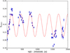 |
Fig. 2. HD 16673 SMWO time series taken with TIGRE. The red line depicts the sinusoidal fit with a period of 309.4 days. |
The result of our Lomb-Scargle analysis is shown in the upper panel of Fig. 3. The GLS periodogram has a significant peak at 309.4 days with a FAP of 5 × 10⁻¹⁵ for this period. In the lower panel of Fig. 3, the window function of our HD 16673 S-index time series is presented, which clearly shows the seasonal sampling of one year. However, this peak at 355 days in the window function is clearly different from the peak in the time series periodogram. We therefore conclude that the GLS period is not influenced by the seasonal sampling and is indeed highly significant.
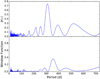 |
Fig. 3. Upper panel: periodogram of the HD 16673 S-index time series. Lower panel: window function of the HD 16673 S-index time series. |
The S-index data, phase-folded with the period of 309.4 days, are shown in Fig. 4. To estimate the amplitude of the variation, we fit the data with a sine function with the most significant period, and the result is shown as a red line in Figs. 2 and 4. We find an amplitude of the variation of 0.0144 in SMWO; after the removal of this variation, the standard deviation of the residuals is reduced to 0.0065.
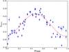 |
Fig. 4. Phase-folded HD 16673 SMWO time series taken with TIGRE. The red line depicts the sinusoidal fit with a period of 309.4 days. |
4.2. HD 49933
HD 49933 is of the spectral type F3V (according to the Simbad database) and has a rotational period of 3.45 days (Mosser et al. 2009). For this star, an indication for a short-term activity cycle of at least 120 days in the CoRoT light curve is reported by García et al. (2010). Furthermore, a Mount Wilson S-index of 0.3 is given for HD 49933 in García et al. (2010). In the upper panel of Fig. 5 we show the TIGRE SMWO-index time series, from which we derive a mean S-index value of 0.213 with a standard deviation of 0.01, clearly lower than the value reported by García et al. (2010). This difference might be due to different S-index calibrations and/or to a long-term trend caused by a long-term activity cycle. In our TIGRE S-index data, a long-term trend is visible (see red line in the upper panel of Fig. 5), suggesting that a part of the S-index difference could be caused by this trend.
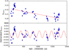 |
Fig. 5. Upper panel: HD 49933 SMWO time series taken with TIGRE. The red line depicts the estimated trend. Lower panel: detrended SMWO time series; the red line depicts the sinusoidal fit with the found period of 219.2 days. |
For the Lomb-Scargle analysis, we detrend our S-index time series (see lower panel of Fig. 5), from which we compute the Lomb-Scargle periodogram plotted in the upper panel of Fig. 6; the window function of our S-index time series is shown in the lower panel of Fig. 6. The highest peak in the periodogram and therefore the most probable period is at 212.2 days, for which we estimate a FAP of 7 × 10⁻⁶. The S-index data are fitted with a sinusoidal curve at the determined period of 212.2 days and the result is depicted as the red line in the lower panel of Fig. 6 and in Fig. 7 for the phase-folded S-index; from the sinusoidal fit we obtain an amplitude of this variation of 0.0063 with a standard deviation of 0.0052.
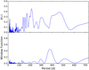 |
Fig. 6. Upper panel: periodogram of the HD 49933 S-index time series. Lower panel: window function of the HD 49933 S-index time series. |
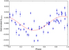 |
Fig. 7. Phase-folded HD 49933 SMWO time series taken with TIGRE. The red line depicts the sinusoidal fit with the found period of 212.2 days. |
However, the periodogram also shows two clear peaks at 170.1 and 465.7 days with a FAP of 6 × 10⁻⁴ and 2 × 10⁻⁴, respectively. To test the significance of the peaks, we performed pre-whitening for the three periods. First, the most probable period of 212.2 days is removed and the Lomb-Scargle analysis of the residuals performed. Here, the peak at 465.7 days vanishes but not the peak at 170.1 days. Next, the 465.7-day period is removed and the residuals are tested. In this case, the 212.2-day period remains, but the peak is no longer significant, while the peak at 170.1 days decreases slightly and a smaller peak at ∼300 days in the periodogram (see lower panel of Fig. 6) becomes the strongest peak in the periodogram of the residuals. From this test, we can conclude that the periods of 212.2 and 465.7 days are not independent. Finally, the 170.1-day period is removed and the peaks at 212.2 and 465.7 days remain. Hence, the 170.1-day period is interesting. It appears that this period is independent of both the 212.2-day and the 465.7-day periods, but to check the significance of this period, a longer and more densely sampled time series is required.
4.3. HD 75332
HD 75332 is of spectral type F7V (Simbad database) with a rotational period of 4.8 days (Vidotto et al. 2014). Baliunas et al. (1995) list HD 75332 with a mean SMWO-index of 0.279 as a variable star without a significant period in the range of 1–25 yr. We obtained a mean SMWO-index of 0.279 with a standard deviation of 0.01, again consistent with the SMWO value listed by Baliunas et al. (1995).
The TIGRE SMWO time series is presented in Fig. 8, and in the upper panel of Fig. 9 we show the periodogram of our TIGRE SMWO time series. This periodogram has two significant peaks, the higher peak being located at 179.9 days with a FAP of 5 × 10⁻¹⁷. The second significant peak is at 349.5 days, which is very close to one year and the sampling-related, seasonal peak at 384.2 days, as seen in the window function (in the lower panel in Fig. 9). We cannot exclude that this second peak may be influenced by the seasonal sampling, so we disregard it.
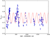 |
Fig. 8. HD 75332 SMWO time series taken with TIGRE; the red line depicts the sinusoidal fit with a period of 179.9 days. |
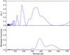 |
Fig. 9. Upper panel: periodogram of the HD 75332 S-index time series. Lower panel: window function of the HD 75332 S-index time series. |
In Fig. 10 the phase-folded TIGRE SMWO data are presented; the S-index data are fitted with a sine function at the main period at 179.9 days and the result of this fit is shown as a red line in Figs. 8 and 10. From this fit, we obtain an amplitude for the periodic variation of 0.0095. Also, it is clear that the fit with the period of 179.9 days describes the data in the first two seasons very well. Finally, when removing the variations from the data we obtain a standard deviation of 0.0073 for the residuals and a pre-whitening test shows no remaining periodic variations. Additionally, we perform a pre-whitening test with the 349.5-day period. Here, the period at 179.9 days remains, but the significance of the peak is reduced significantly.
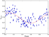 |
Fig. 10. Phase-folded HD 75332 SMWO time series taken with TIGRE; the red line depicts the sinusoidal fit with a period of 179.9 days. |
4.4. HD 100563
The spectral type of HD 100563 is F5.5V (Simbad database). A rotation period of 7.73 days was listed in Hempelmann et al. (2016), albeit with low significance (1σ) obtained from TIGRE data taken from 2013 to 2014. Baliunas et al. (1995) list HD 100563 with a mean SMWO-index of 0.202 and without a significant period. In the upper panel of Fig. 11, we show the SMWO time series taken with TIGRE; we find a mean SMWO-index of 0.195 with a standard deviation of 0.0063, slightly lower than the value listed in Baliunas et al. (1995).
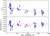 |
Fig. 11. HD 100563 SMWO time series taken with TIGRE. The red line depicts the sinusoidal fit with a period of 222.3 days. |
However, we see a small trend in our S-index data, which might explain this small difference; the detrended time series is shown in the lower panel of Fig. 11. After detrending we perform the Lomb-Scargle analysis and present the result in the upper panel of Fig. 13, while the lower panel of Fig. 13 shows the window function of this time series. The highest peak in the GLS periodogram is at a period of 222.3 days with a formal FAP of only 1 × 10⁻³. The FAP of HD 100563 is small compared to the other three objects in this work. Following the classification of the FAP grade by Baliunas et al. (1995), the cycle is only “fair”. We therefore consider this result as simply an indication of a short-term cycle. In Fig. 12, we show the phase-folded TIGRE S-index data together with a sine function fit to the data (using the period of 222.3 days); in Figs. 11 and 12 these fit results are depicted with the red line. For the amplitude of this variation we obtain 0.0033 and after the removal of the cycle, the standard deviation of the residuals is 0.0042.
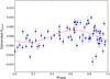 |
Fig. 12. Phase-folded HD 100563 SMWO time series taken with TIGRE. The red line depicts the sinusoidal fit with a period of 222.3 days. |
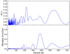 |
Fig. 13. Upper panel: periodogram of the HD 100563 S-index time series. Lower panel: window function of the HD 100563 S-index time series. |
5. Summary and conclusions
In this paper we present the S-index time series of four F-type stars observed with the TIGRE telescope. In each of these time series we find a significant periodic signal, which we interpret as a short-term magnetic cycle; the amplitudes lie between 0.003 and 0.015 in S-index values.
With the detections of three more short-term cycles and one candidate, in addition to the already known cycle of τ Boo, we conclude that such short-term activity cycles appear to be a common and possibly typical phenomenon in F-type stars. The cycle lengths of the four found activity cycles are between 0.5 and 1 year, so the 120-day short-term activity cycle in τ Boo is still the shortest known, albeit by no means exceptional.
Furthermore, we find that in these four F-stars the amplitude of the cycle is not as large as commonly found with long-period (10+ years), solar-type cyclic activity. Therefore these short-term cycles may contribute to further activity with a large spectrum of variability in the time domain, or the observed smaller amplitude may be inherent to this type of short-term cycle.
The currently available sample is clearly too small to draw any statistically significant conclusions, but it did not escape our attention that in our four stars rotation periods and cycle lengths are roughly proportional. On the other hand, such a direct comparison does not hold in its extension to solar-type stars, where the cycle periods are more than an order of magnitude longer. Brandenburg et al. (2017) derive a relation between the cycle length and rotation period using the convective turnover time as a factor in their relation. The convective turnover time depends on the colour index B − V or rather Teff, and therefore one can assume a B − V dependence between the cycle length and the rotation period.
In this respect, we find the theoretical prediction of Brandenburg et al. (2017), that is, that both long and short period cycles could co-exist, very interesting. In Fig. 14, we show the cycle period versus the rotational period; the blue data points (Sun with a diamond) are depicted; the data are taken from Brandenburg et al. (2017, Table 3) for F- and G-type stars of the so-called short inactive branch. The short-term cycles found is this work with the corresponding rotational periods mentioned in the text, and also the cycle and rotational period of τ Boo taken from Mittag et al. (2017) are all displayed as red points in Fig. 14; except HD 100563 which is shown as red square. We see from Fig. 14 that the short-term cycles (red points) seem to be consistent with the short-term cycle branch from Brandenburg et al. (2017). We also note that ι Hor (HD 17051) is included in the Brandenburg sample (last blue data point at the low period tail) and fits in the general trend. We therefore conclude that for the study of magnetic activity of solar-like stars in a wider context, and to aid dynamo theory modelling, Ca II monitoring of F-type stars appears to be a rewarding task, which is perfectly suited for a robotic telescope like TIGRE.
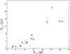 |
Fig. 14. Blue data points taken from Brandenburg et al. (2017; Table 3) (Sun with a diamond) for F- and G-type stars referred to as the short inactive branch. The red data point are labelled the short-term cycles found in this work (the corresponding rotational periods are mentioned in the text) including the cycle and rotational period of τ Boo taken from Mittag et al. (2017). The red square data point marks HD 100563 where the significance of the period are comparable low and therefore, we consider this object only as a candidate for a short-term activity cycle. |
Acknowledgments
This research has made use of the VizieR catalogue access tool, CDS, Strasbourg, France. The original description of the VizieR service was published in A&AS 143, 23.
References
- Baliunas, S. L., Horne, J. H., Porter, A., et al. 1985, ApJ, 294, 310 [NASA ADS] [CrossRef] [Google Scholar]
- Baliunas, S. L., Donahue, R. A., Soon, W. H., et al. 1995, ApJ, 438, 269 [NASA ADS] [CrossRef] [Google Scholar]
- Baliunas, S. L., Henry, G. W., Donahue, R. A., Fekel, F. C., & Soon, W. H. 1997, ApJ, 474, L119 [NASA ADS] [CrossRef] [Google Scholar]
- Brandenburg, A., Mathur, S., & Metcalfe, T. S. 2017, ApJ, 845, 79 [NASA ADS] [CrossRef] [Google Scholar]
- ESA. 1997, in The HIPPARCOS and TYCHO Catalogues. Astrometric and Photometric Star Catalogues Derived from the ESA HIPPARCOS Space Astrometry Mission, ESA Special Publ., 1200 [Google Scholar]
- García, R. A., Mathur, S., Salabert, D., et al. 2010, Science, 329, 1032 [NASA ADS] [CrossRef] [PubMed] [Google Scholar]
- Gorynya, N. A., & Tokovinin, A. 2018, MNRAS, 475, 1375 [NASA ADS] [CrossRef] [Google Scholar]
- Hempelmann, A., Mittag, M., Gonzalez-Perez, J. N., et al. 2016, A&A, 586, A14 [NASA ADS] [CrossRef] [EDP Sciences] [Google Scholar]
- Mengel, M. W., Fares, R., Marsden, S. C., et al. 2016, MNRAS, 459, 4325 [NASA ADS] [CrossRef] [Google Scholar]
- Metcalfe, T. S., Basu, S., Henry, T. J., et al. 2010, ApJ, 723, L213 [NASA ADS] [CrossRef] [Google Scholar]
- Mittag, M., Hempelmann, A., González-Pérez, J. N., & Schmitt, J. H. M. M. 2010, Adv. Astron., 2010, 101502 [NASA ADS] [CrossRef] [Google Scholar]
- Mittag, M., Schröder, K.-P., Hempelmann, A., González-Pérez, J. N., & Schmitt, J. H. M. M. 2016, A&A, 591, A89 [NASA ADS] [CrossRef] [EDP Sciences] [Google Scholar]
- Mittag, M., Robrade, J., Schmitt, J. H. M. M., et al. 2017, A&A, 600, A119 [NASA ADS] [CrossRef] [EDP Sciences] [Google Scholar]
- Mittag, M., Hempelmann, A., Fuhrmeister, B., Czesla, S., & Schmitt, J. H. M. M. 2018, Astron. Nachr., 339, 53 [NASA ADS] [CrossRef] [Google Scholar]
- Mosser, B., Baudin, F., Lanza, A. F., et al. 2009, A&A, 506, 245 [NASA ADS] [CrossRef] [EDP Sciences] [Google Scholar]
- Piskunov, N. E., & Valenti, J. A. 2002, A&A, 385, 1095 [NASA ADS] [CrossRef] [EDP Sciences] [Google Scholar]
- Schmitt, J. H. M. M., & Mittag, M. 2017, A&A, 600, A120 [NASA ADS] [CrossRef] [EDP Sciences] [Google Scholar]
- Schmitt, J. H. M. M., Schröder, K.-P., Rauw, G., et al. 2014, Astron. Nachr., 335, 787 [NASA ADS] [CrossRef] [Google Scholar]
- Schröder, K.-P., Mittag, M., Hempelmann, A., González-Pérez, J. N., & Schmitt, J. H. M. M. 2013, A&A, 554, A50 [NASA ADS] [CrossRef] [EDP Sciences] [Google Scholar]
- Schwabe, H. 1844, Astron. Nachr., 21, 233 [NASA ADS] [CrossRef] [Google Scholar]
- Vidotto, A. A., Gregory, S. G., Jardine, M., et al. 2014, MNRAS, 441, 2361 [NASA ADS] [CrossRef] [Google Scholar]
- Wilson, O. C. 1978, ApJ, 226, 379 [NASA ADS] [CrossRef] [Google Scholar]
- Zechmeister, M., & Kürster, M. 2009, A&A, 496, 577 [NASA ADS] [CrossRef] [EDP Sciences] [Google Scholar]
All Tables
All Figures
|
Fig. 1. Ratio of the mean TIGRE S-data obtained from the reduction pipelines. |
| In the text | |
|
Fig. 2. HD 16673 SMWO time series taken with TIGRE. The red line depicts the sinusoidal fit with a period of 309.4 days. |
| In the text | |
|
Fig. 3. Upper panel: periodogram of the HD 16673 S-index time series. Lower panel: window function of the HD 16673 S-index time series. |
| In the text | |
|
Fig. 4. Phase-folded HD 16673 SMWO time series taken with TIGRE. The red line depicts the sinusoidal fit with a period of 309.4 days. |
| In the text | |
|
Fig. 5. Upper panel: HD 49933 SMWO time series taken with TIGRE. The red line depicts the estimated trend. Lower panel: detrended SMWO time series; the red line depicts the sinusoidal fit with the found period of 219.2 days. |
| In the text | |
|
Fig. 6. Upper panel: periodogram of the HD 49933 S-index time series. Lower panel: window function of the HD 49933 S-index time series. |
| In the text | |
|
Fig. 7. Phase-folded HD 49933 SMWO time series taken with TIGRE. The red line depicts the sinusoidal fit with the found period of 212.2 days. |
| In the text | |
|
Fig. 8. HD 75332 SMWO time series taken with TIGRE; the red line depicts the sinusoidal fit with a period of 179.9 days. |
| In the text | |
|
Fig. 9. Upper panel: periodogram of the HD 75332 S-index time series. Lower panel: window function of the HD 75332 S-index time series. |
| In the text | |
|
Fig. 10. Phase-folded HD 75332 SMWO time series taken with TIGRE; the red line depicts the sinusoidal fit with a period of 179.9 days. |
| In the text | |
|
Fig. 11. HD 100563 SMWO time series taken with TIGRE. The red line depicts the sinusoidal fit with a period of 222.3 days. |
| In the text | |
|
Fig. 12. Phase-folded HD 100563 SMWO time series taken with TIGRE. The red line depicts the sinusoidal fit with a period of 222.3 days. |
| In the text | |
|
Fig. 13. Upper panel: periodogram of the HD 100563 S-index time series. Lower panel: window function of the HD 100563 S-index time series. |
| In the text | |
|
Fig. 14. Blue data points taken from Brandenburg et al. (2017; Table 3) (Sun with a diamond) for F- and G-type stars referred to as the short inactive branch. The red data point are labelled the short-term cycles found in this work (the corresponding rotational periods are mentioned in the text) including the cycle and rotational period of τ Boo taken from Mittag et al. (2017). The red square data point marks HD 100563 where the significance of the period are comparable low and therefore, we consider this object only as a candidate for a short-term activity cycle. |
| In the text | |
Current usage metrics show cumulative count of Article Views (full-text article views including HTML views, PDF and ePub downloads, according to the available data) and Abstracts Views on Vision4Press platform.
Data correspond to usage on the plateform after 2015. The current usage metrics is available 48-96 hours after online publication and is updated daily on week days.
Initial download of the metrics may take a while.