| Issue |
A&A
Volume 621, January 2019
|
|
|---|---|---|
| Article Number | A109 | |
| Number of page(s) | 12 | |
| Section | Stellar structure and evolution | |
| DOI | https://doi.org/10.1051/0004-6361/201833779 | |
| Published online | 17 January 2019 | |
Diversity of supernovae and impostors shortly after explosion⋆
Trinity College Dublin, The University of Dublin, College Green, Dublin, Ireland
e-mail: This email address is being protected from spambots. You need JavaScript enabled to view it.
, This email address is being protected from spambots. You need JavaScript enabled to view it.
Received:
5
July
2018
Accepted:
21
November
2018
Abstract
Observational surveys are now able to detect an increasing number of transients, such as core-collapse supernovae (SN) and powerful non-terminal outbursts (SN impostors). Dedicated spectroscopic facilities can follow up these events shortly after detection. Here we investigate the properties of these explosions at early times. We use the radiative transfer code CMFGEN to build an extensive library of spectra simulating the interaction of supernovae and their progenitor’s wind or circumstellar medium (CSM). We have considered a range of progenitor mass-loss rates (Ṁ = 5 × 10⁻⁴−10−2 M⊙ yr−1), abundances (solar, CNO-processed, and He-rich), and SN luminosities (L = 1.9 × 10⁸ − 2.5 × 10¹⁰ L⊙). The models simulate events approximately one day after explosion, and we assume a fixed location of the shock front as Rin = 8.6 × 1013 cm. We show that the large range of massive star properties at the pre-SN stage causes a diversity of early-time interacting SN and impostors. We identify three main classes of early-time spectra consisting of relatively high-ionisation (e.g. He II and O VI), medium-ionisation (e.g. C III and N III), and low-ionisation lines (e.g. He I and Fe II/III). They are regulated by L and the CSM density. Given a progenitor wind velocity υ∞, our models also place a lower limit of Ṁ ≳ 5 × 10⁻⁴ (υ∞/150 km s−1) M⊙ yr−1 for detection of CSM interaction signatures in observed spectra. Early-time SN spectra should provide clear constraints on progenitors by measuring H, He, and CNO abundances if the progenitors come from single stars. The connections are less clear considering the effects of binary evolution. Nevertheless, our models provide a clear path for linking the final stages of massive stars to their post-explosion spectra at early times, and guiding future observational follow-up of transients with facilities such as the Zwicky Transient Facility.
Key words: supernovae: general / stars: massive / surveys / stars: winds / outflows / stars: mass-loss / stars: evolution
The spectral data are also available at the CDS via anonymous ftp to cdsarc.u-strasbg.fr (130.79.128.5) or via http://cdsarc.u-strasbg.fr/viz-bin/qcat?J/A+A/621/A109, at www.tcd.ie/Physics/research/groups/groh/sn1day/ and at WISeREP via https://wiserep.weizmann.ac.il
© ESO 2019
1. Introduction
Most stars more massive than ≈8 M⊙ end their lives as supernovae (SNe). While the observed diversity in supernovae should reflect the variety of massive star progenitors, the exact links are not fully established.
There are various complementary methods to determine the progenitors of SNe. For a number of events, progenitors have been identified in pre-explosion images (Smartt 2015; Van Dyk 2017, and references therein). However, in general only limited photometric observations are available. SN lightcurves and spectra can give an indication of the ejecta mass, explosion energy and amount of synthesised Ni56, which can then be linked to the progenitor properties such as its initial mass (Woosley & Weaver 1986). For interacting events, lightcurves can be used to constrain some of the atmosphere or wind properties as well (e.g. Moriya et al. 2014), which also map to a progenitor class. The environments of transients constrain the ages and metallicities of the nearby stellar populations and of the progenitor itself (Anderson et al. 2015; Xiao et al. 2019).
In addition to the techniques discussed above, early-time or “flash” spectroscopy provides substantial information on SN progenitors (Gal-Yam et al. 2014; Groh 2014; Smith et al. 2015; Gräfener & Vink 2016; Khazov et al. 2016; Yaron et al. 2017). Throughout their evolution, massive stars have high mass-loss rates (Ṁ ≥ 10−6 M⊙ yr−1; Smith 2014) that form a circumstellar medium (CSM). When the stars undergo an explosive event, the fast ejecta (vej ≈ 10 000 km s−1) will crash into the slow CSM (υ∞ ≈ 10 − 1000 km s−1) and the kinetic energy of the SN ejecta is converted to radiation. The radiation then photo-ionises the CSM, which becomes optically thick and the photosphere is formed in the CSM for a period of time ranging from days to a few years, depending on the CSM density and extension. Most optical emission lines such as Hα are formed by recombination in a medium under photoionisation equilibrium. Therefore, a spectrum obtained at this stage should reflect the CSM density, velocity, and abundance profiles (Chevalier & Fransson 1994; Chugai 2001; Dessart et al. 2009, 2015; Groh 2014). Using this technique, Groh (2014) suggested that the progenitor of SN 2013cu is consistent with a luminous blue variable (LBV) or a yellow hypergiant (YHG; see also Gräfener & Vink 2016). Similarly Shivvers et al. (2015) found that the progenitor of SN 1998S could have been an LBV, YHG or massive YHG. Yaron et al. (2017) proposed a red supergiant (RSG) as the progenitor of SN 2013fs (see also Dessart et al. 2017).
Due to the presence of a dense CSM, these SN show a “wind breakout” (Moriya et al. 2018) rather than a classical shock breakout. In this paper we cover a large range of mass-loss rates, which results in a large range of CSM densities. Therefore some of the SNe may show long-term interaction and if observed would be classified as type IIn SNe. However, others may show short-term interaction that may be missed by the observers if not detected early enough and would be classified as a type IIP, IIL, or IIb, based on the late-time spectra.
Since early-time spectroscopic observations and modelling of supernovae probe the most final stages of the star, they are a useful tool not only for linking supernovae to their progenitors but also in improving our knowledge of late-time massive star evolution. This is due to the fact that accurate observations of massive stars at late stages are impaired by their low numbers and sometimes dust-enshrouded surroundings, while modelling their evolution shows large dependencies on mass-loss, metallicities, rotational velocities (Ekström et al. 2012; Georgy et al. 2013), magnetic fields (Petit et al. 2017), and interaction with a companion (Podsiadlowski et al. 1992; Langer 2012; Eldridge et al. 2017). These factors play an important role in determining the “explodability” of a massive star (e.g., Renzo et al. 2017; Sukhbold et al. 2018), and the type and mass of the SN remnant (Fryer & Kalogera 2001; Heger et al. 2003; O’Connor & Ott 2011) on which our understanding of gravitational wave observations rely (Abbott et al. 2016, 2017; Belczynski et al. 2016).
It is clear that there is a need for improved understanding of the final stages of massive star evolution and their links to SNe. In this article we present our grid of models that simulate the spectra of supernovae shortly after explosion (approximately one day). Observations on a timescale of a day offer a good compromise between the time necessary to obtain transient spectra and the sensitivity to low-density CSM. We have explored a wide range of progenitor mass-loss rates, surface abundances, and explosion luminosities to investigate the spectral diversity of SNe at early times. The set of models discussed here is part of an extensive library and it is publicly available to the community. Our models complement the extensive observational efforts that have established the diversity of these events (e.g., Smith et al. 2011; Taddia et al. 2013; Khazov et al. 2016), and extend previous computational efforts (Dessart et al. 2009, 2017; Groh 2014) to a large range of CSM abundances and densities. Given the rapid increase in the number of observed events with the advent of wide-field surveys such as the Zwicky Transient Facility (ZTF), our public library of models provides the community with a tool to estimate progenitor properties in a timely fashion.
2. CMFGEN radiative transfer modelling
We used the non-local thermodynamical equilibrium radiative transfer code CMFGEN (Hillier & Miller 1998) to compute radiative transfer models of interacting SN and SN impostors at early stages after the explosion. In our setup, the code simulates the transport of radiative energy generated by the conversion of the kinetic energy of the supernova ejecta as it shocks against the progenitor’s wind or CSM. The code requires a number of input physical parameters, such as the location of the inner boundary (Rin), luminosity of the event (L), and the progenitor’s mass-loss rate Ṁ, wind terminal velocity υ∞ and surface abundances. We refer to Groh (2014), Shivvers et al. (2015), and Yaron et al. (2017) for further details on the implementation.
We assume a steep density scale height with a gradient of 0.008 Rin for the shocked region connected smoothly to an unclumped stationary wind which has a density profile ρ ∝ r−2 to represent the wind or CSM of the progenitor. We assume diffusion approximation at Rin and adjust the density to have a Rosseland optical depth τRoss ≳ 100 at Rin. We have ensured that the photosphere (where τRoss = 2/3) is located in the progenitor wind for the radiation field and hydrodynamics of the inner region to minimally affect the spectra. We choose Rin = 8.64 × 1013 cm to correspond to the location of the shock front at t ≃ 1 day after explosion, assuming a constant SN ejecta velocity of 10 000 km s−1.
For a given value of Rin and L we can use the Stefan-Boltzmann law to define a flux temperature at the inner boundary:
 (1)
(1)
where σ is the Stefan-Boltzmann constant. Therefore Tin is affected by both Rin and L and a change in either parameter could modify the spectral morphology. In this paper we use a single Rin value for all models, both because we focus on a specific time after explosion (about one day) and to minimise the number of parameters that vary in our grid of models. We stress that additional models would be needed to explore the spectral morphology at times much larger than one day after explosion.
We compute models with L = 1.9 × 10⁸ − 2.5 × 10¹⁰ L⊙, Ṁ = 5 × 10⁻⁴−10−2 M⊙ yr−1, υ∞ = 150 km s−1 and three sets of abundances (solar, CNO-processed, and He-rich). We also keep the same υ∞ for all models in Figs. 1 and 2 to minimise the number of parameters affecting the spectral morphology, and to avoid making a connection between quiescent wind parameters and pre-SN outflow properties. We discuss the effects of lower values of υ∞ in Sect. 3. The models include Si, P, S and Fe at solar abundances. Table 1 lists the model properties.
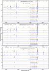 |
Fig. 1. CMFGEN optical spectra of SNe interacting with their progenitor’s wind at early times for solar (top panel), CNO-processed (middle panel), and He-rich abundances (bottom panel). The models have been convolved with a Gaussian kernel of Δv = 300 km s−1 (resolving power R ≈ 1000), continuum normalised, and shifted for clarity. The labels indicate the adopted values of Ṁ3 (10−3 M⊙ yr−1) and L9 (109 L⊙), and the strongest spectral lines are identified. |
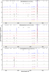 |
Fig. 2. CMFGEN optical spectra of SNe interacting with their progenitor’s wind at early times for solar (top panel), CNO-processed (middle panel), and He-rich abundances (bottom panel). The models have been convolved with a Gaussian kernel of Δv = 300 km s−1 (resolving power R ≈ 1000), continuum normalised, and shifted for clarity. All the models in this figure have Ṁ = 3 × 10⁻³ M⊙ yr−1. The labels indicate the adopted values of L9 (109 L⊙), and the strongest spectral lines are identified. |
Physical properties of the CMFGEN radiative transfer simulations.
While CMFGEN can produce arbitrarily high resolution spectra, spectroscopic observations of SNe usually have low to medium resolution (30 ≤ Δv ≤ 2000 km s−1), therefore Fig. 1 shows our spectra convolved with a Gaussian kernel of Δv = 300 km s−1 (resolving power R ≃ 1000). The high-resolution spectra can be found in Appendix A and in our online database.
Our models have several approximations to study the radiative transfer problem in interacting SNe. First, we do not solve for the time-dependent radiation hydrodynamics of the CSM. For a detailed discussion on these effects, see Dessart et al. (2017). Our models are valid when the photosphere forms in the CSM, during which radiative equilibrium is still a reasonable approximation (Dessart et al. 2009; Groh 2014). In addition, ignoring time-dependent effects allows the models to complete in a reasonable amount of time, which is crucial for producing a large grid of models that can fit the observations as is the goal of this paper. Second, we compute models with various L and Ṁ, although the time variation of L should depend on the diffusion timescale, and thus Ṁ. We note that the diffusion timescale is ≈10 h for Ṁ = 10−2 M⊙ yr−1 and υ∞ = 150 km s−1 (Chevalier & Irwin 2011), and that the same Ṁ can lead to a variety of L depending on the explosion energies (Moriya et al. 2011), asymmetry of the CSM, or clumping or porosity in the CSM. Thirdly, we assume a spherically-symmetric CSM, which may not be the case for some SNe (Smith 2017).
3. Diversity of interacting supernovae and impostors
Our models show that the large range of physical parameters of massive stars before death produces a significant diversity of spectral morphologies in SNe. Broadly, we identify three main morphologies in transient optical spectra produced shortly after explosion in our solar abundance models at a medium resolution of R = 1000 (Figs. 1 and 2, top panel).
-
High-ionisation spectra, characterised by O VI, He II, N V, and H I emission lines. This morphology appears at high L (> 6.3 × 10⁹ L⊙) and resembles SN 2013fs;
-
Medium-ionisation spectra, with strong He II, C III, N III, N IV, C IV, and He I emission. These are seen at L between 3.9 × 10⁸ − 3.1 × 10⁹ L⊙ and might correspond to a solar-abundance version of SN 1998S observed at early times;
-
Low-ionisation spectra, with H I, He I, and Fe II lines with P Cygni profiles. The models with high Ṁ show [O III] and [N II]. This spectral morphology is present at relatively low L (≈1.9 × 10⁸ L⊙) and resembles classical SN IIn, such as SN 1994W, as they would have been seen at early times.
These morphologies arise from the dominant effect of L on Tin, and thus on the ionisation structure of the CSM, and the strength of spectral lines from different ions. An increase in L produces a more ionised CSM, and we see a shift towards lines of high ionisation stages. Perhaps surprisingly, the H I emission decreases with increasing L, because the recombination rate coefficient decreases with the increase in the electron temperature (Te) that is seen in high L models. Therefore, the L = 1.9 × 10⁸ L⊙ models show the strongest H α emission for a given Ṁ (Figs. 1 and 2).
The spectral classes discussed above are meant to underline the effects of L on the spectrum and guide the observers. However the changes on the spectrum are rather continuous, with cases falling in between the three described morphologies. One such example is the model with L = 6.3 × 10⁹ L⊙ which shows C IV emission lines seen mostly in the medium ionisation case, but also shows N V emission which belongs to the highly ionised spectral morphology (Fig. 2). Additionally, the abundances and the mass-loss rate will also play a role in which species are observable for each luminosity case.
We find that changing the Ṁ of the progenitor affects the ionisation structure of the CSM as well, albeit to a lower degree than changing L (we need Ṁ ≳ 0.1 M⊙ yr−1 to generate a significant recombination of the CSM). For a given L, an increase in Ṁ leads to stronger emission in all lines because of the increased density of the CSM. Also, since the density increases while the input of energy at the base of the wind is constant, the ionisation structure shifts towards less ionised ions (Fig. 1). This is reflected in the ionisation stages seen in the spectra, for example higher N III/N IV and C III/C IV ratios for high values of Ṁ.
The differences in the spectra due to changes in abundances are strong. In both CNO-processed and He-rich sets of models, we identify the same trend of spectral morphologies with respect to L and Ṁ discussed above. As expected, we find that the strength of spectral lines change monotonically according to the abundance of that element in the parameter range explored here. Our models with abundances corresponding to CNO-processed material show stronger N emission, weak C and no O lines (Fig. 1, middle panel). The high-ionisation models show no O VI even for high L. Medium-ionisation models develop strong N IV, making them similar to SN 2013cu (Gal-Yam et al. 2014; Groh 2014). Low-ionisation models are not substantially affected in the models displayed here, although weak N II lines could appear at certain combinations of L and Ṁ. The H α line is weaker in CNO-processed models compared to the corresponding solar abundance model. This is caused by the higher Te of the CNO-processed models, which stems from the decrease of radiative losses in the CSM due to lower C and O abundances. The highest Ṁ models show the largest difference between the two different abundances. The decrease in emissivity due to the increase in Te strongly affects the He II emission as well, and weakly the He I emission.
The He-rich models show a substantial decrease in the ratio between H α and He II lines compared to the CNO-processed models (Fig. 1, bottom panel). This is caused by the diminished H abundance. As for the CNO-processed models, almost no O or C emission are present in any of the He-rich models. Although the decrease in the H abundance also lowers the opacity and raises Te, these changes do not substantially impact the CSM ionisation structure.
The H α and He II lines are the most degenerate with respect to Ṁ and L. However, if both lines are detected in the spectrum, their abundances can be well constrained if the observations cover the optical range from 3700–7500 Å, and either flux-calibrated spectra or multi-band photometry are available. As Fig. 1 shows, this allows a determination of the ionisation structure of the wind, which breaks the degeneracy. For example, while both a solar abundance, high L model and a He-rich, low L model can have similar H α strengths, the He II line will be much stronger for a higher He abundance. Analogously, He I lines can be also employed.
The Fe abundance is in general difficult to constrain from optical spectra alone. It could be determined from the Fe II lines present in the optical spectrum of some of the low-L models. In contrast, the UV region is extremely populated by Fe lines (Fig. A.1) which provides a tool for determining the metallicities if UV data are available or for high-redshift SNe.
Additional degeneracies appear due to a larger range of possible values of υ∞ for events observed at low spectral resolution. This leads to an increased range of possible values of Ṁ because of the mass continuity equation (ρ ∝ Ṁ/υ∞). Figure 3 shows solar abundance models with L = 1.5 × 10⁹ L⊙, υ∞ = 15 km s−1, and resolution of R = 1000 together with the corresponding υ∞ = 150 km s−1 models from Fig. 1. Most of our models with the same density profile but different values of υ∞ and Ṁ are barely distinguishable at R = 1000 (but see Gräfener & Vink 2016). Noticeable changes appear only for models with high CSM densities (Ṁ = 10−2 M⊙ yr−1). In this case, a change in υ∞ can result in an overlap of neighbouring spectral lines, which may lead to temperature changes observable in the N III/N IV and C III/C IV ratios.
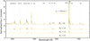 |
Fig. 3. CMFGEN optical spectra of SNe interacting with their progenitor’s wind at early times for progenitors with υ∞ = 150 km s−1 (models from Fig. 1; black) and with υ∞ = 15 km s−1 (overplotted on the corresponding high υ∞ models; yellow). The models have been convolved with a Gaussian kernel of Δv = 300 km s−1 (resolving power R ≈ 1000), continuum normalised, and shifted for clarity. The labels indicate the adopted values of Ṁ3 (10−3 M⊙ yr−1), and the strongest spectral lines are identified. All the models in this figure have solar abundances and L = 1.5 × 10⁹ L⊙. |
4. Linking supernovae to their progenitors
Early-time spectroscopy of SN offers three valuable clues on the nature of their progenitors: Ṁ, υ∞, and abundances. However, theoretical models in recent years suggest a scenario in which the outflow properties and mass-loss mechanisms at the pre-SN stage (e.g. Fuller 2017, and references therein) are markedly different than those seen in post-MS massive stars in the Galaxy and Magellanic Clouds (Smith 2017), which are expected to be at the He-core burning stage. Thus, linking Ṁ and υ∞ derived from early-time SNe to classes of massive stars characterised by those values may be misleading. This is highlighted by our lower limit of Ṁ ≳ 5 × 10⁻⁴(150 km s−1/υ∞) M⊙ yr −1 for detection of clear spectroscopic evidence of SN-CSM interaction. This lower limit is higher than the typical Ṁ of almost all massive stars in the local Universe, except for selected LBVs such as Eta Car (Groh et al. 2012) and others during S-Dor type outbursts (Smith 2014).
For this reason, progenitor surface abundances may offer a more direct connection between pre- and post-SN spectra if abundances can be used as a proxy for the initial mass. This is generally the case for single star evolution (e.g. Groh et al. 2013). Binary evolution produces significantly more possible outcomes (see e.g. Eldridge et al. 2017) because of the large range of inferred initial orbital periods and mass ratios of massive binaries (Sana et al. 2012; Moe & Di Stefano 2017). Below we discuss some of the possible evolutionary connections of single and binary stars to our early-time spectral morphology, and the key spectroscopic diagnostics that could be used to constrain SN progenitors.
Low-mass RSGs correspond to single star initial masses of 8–15 M⊙, or less massive mass gainers in binary systems. These stars retain most of their massive H envelope, with weak or no CNO processed material at the surface. These progenitors would give rise to early-time post-explosion spectra resembling our first set of models (Figs. 1 and 2, top panel). They should be identifiable using O VIλλ3811, 3834 (high L), or C IIIλ5697, C IVλλ5801, 5811 lines and N IIIλλ4634, 4640 (medium L), or C IIIλλ4647, 4650 (low L).
Massive RSGs, YHGs, BSGs, LBVs, and WN stars correspond to single star initial masses of 15–30 M⊙. A range of initial periods should produce mass gainers, donors, and merger products that would be consistent with these classes of progenitors. They exhibit CNO processed material at the surface as a result of rotational mixing, mass-loss, and/or binary interaction, with variable degree of H envelope stripping. They should show no O VIλλ3811, 3834 at high L, possess N IVλλ4058, 7109, 7122 and N IIIλλ4634, 4640 (medium L), and the C IIIλ5697 and C IVλλ5801, 5811 lines should be absent. The ratio between He II and H lines should provide a reliable estimate of the H and He abundances, and thus on the nature of the progenitor. Higher He/H ratios favour late WN progenitors (these progenitors would show an enrichment of both N and He in their surface abundances and would produce post-explosion spectra similar to our third set of models shown in Figs. 1 and 2, bottom panel), while mild He enrichment would be more consistent with RSGs and BSGs (their early-time post-explosion spectra would correspond to our second set of models in Figs. 1 and 2, middle panel). LBVs show intermediate He enrichment (∼0.65 by mass).
We stress that the mass ranges and evolutionary scenarios above are model dependent and not comprehensive, in particular for binary evolution. In the single-star scenario, early-time SN spectra should provide clear constraints on progenitors by measuring H, He, and CNO abundances.
5. Implications on supernova impostors
It is important to highlight that our models do not assume a terminal explosion as the source of energy at the base of the CSM. Because of that, they can also be applied to the class of SN impostors and intermediate transients. SN impostors are eruptive events that resemble low luminosity SNe, but are instead non-terminal explosions of massive stars (Van Dyk et al. 2000).
It is well known that SN impostors show large spectral diversity, with some events exhibiting “hot” spectra and others “cool” spectra (Smith 2010). While the models presented in this paper do not reach the lowest luminosities of SN impostors, they could be scaled down to reproduce SN impostors’ spectra. To keep a similar Tin at low luminosities, the inner radius would need to also be decreased according to Eq. (1). To maintain the optical depth structure and line luminosities constant, Ṁ would also have to be scaled using the relation Ṁ ∝ L3/4 × υ∞ (e.g. Gräfener & Vink 2016).
Some of our low Tin models do qualitatively resemble known “hot” SN impostors such as SN 1997bs (Van Dyk et al. 2000), SN 2000ch (Wagner et al. 2004), SN 2002bu (Smith et al. 2011) or SN 2009ip (Smith et al. 2010). When early-time observations of SN impostors become routinely available, our models should be able to reproduce the morphology and physical conditions of these events, allowing the determination of progenitor abundances and CSM properties. We will defer to future work an extension of the models to reproduce cool SN impostors.
6. Observational challenges
Our original CMFGEN models have arbitrarily high spectral resolution. However, spectroscopic observations of transients typically have low to medium resolution due to the need for fast spectroscopic follow-up of faint events. This is a continuing trend even with new surveys such as ZTF (Bellm & Kulkarni 2017), which will employ the Double Spectrograph on the Palomar 200″ (resolving power of R ≈ 1000 − 10 000), or the Spectral Energy Distribution Machine (R ≈ 100, Blagorodnova et al. 2018) on the Palomar 60″ telescope. For this reason, we have convolved our spectra with a Gaussian kernel of Δv = 1000 km s−1, corresponding to a resolving power R ≈ 300, to account for the lower end of spectrograph resolutions. Figure 4 shows the low-resolution spectra for the models in Fig. 1. It can be easily seen by comparing Figs. 1 and 4 that the main trends identified in the higher resolution spectra and described in the text can still be observable at lower resolution. However, when fitting observed events, the errors will increase as differences between spectra will be harder to disentangle. This can be problematic especially for events with spectra characterised by medium-ionisation lines.
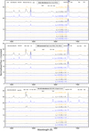 |
Fig. 4. Low-resolution (Δv = 1000 km s−1, R ≈ 300) CMFGEN optical spectra of SNe interacting with their progenitor’s wind at early times for solar (top panel), CNO-processed (middle panel), and He-rich abundances (bottom panel). The models have been continuum normalised and shifted for clarity. The labels indicate the adopted values of Ṁ3 (10−3 M⊙ yr−1) and L9 (109 L⊙), and the strongest spectral lines are identified. |
7. Summary and conclusions
In this paper we have presented a systematic investigation of spectra that simulate SN interacting with their progenitor’s wind approximately one day after explosion. We have covered a large range of SN luminosities (L = 1.9 × 10⁸ − 2.5 × 10¹⁰ L⊙), progenitor mass-loss rates (Ṁ = 5 × 10⁻⁴−10−2 M⊙ yr−1), and progenitor’s surface abundance scenarios (solar, CNO-processed, and He-rich). We summarise our main results below.
-
For the luminosity range considered here the early-time spectra can be classified in three main categories based on ionisation levels. Low-ionisation spectra show mainly H I and He I lines. In the medium-ionisation case C III or N III lines are present, while high-ionisation spectra contain He II, N V or O V/VI lines.
-
Our models show that progenitors with mass-loss rates lower than Ṁ = 5 × 10⁻⁴ (υ∞/150 km s−1) M⊙ yr−1 will not show detectable interaction signatures in the post-explosion spectra.
-
Because of the unknown nature of pre-explosion mass loss, it is challenging to connect CSM densities to different progenitor types. On the other hand, changes in the surface abundances of the progenitors have observable effects on the early-time post-explosion spectra. Early-time SN spectra thus provide constraints on progenitors by measuring H, He, and CNO abundances if the progenitors come from single stars. The connections are less clear considering the effects of binary evolution.
-
The effects discussed above are also observable in low resolution spectra, hence they could be used for linking SN to their progenitors. However, low resolution spectra may yield higher errors in the parameter determinations due to the poorer constraints on the CSM velocity and progenitor’s mass-loss rate.
-
The spectra presented in this paper can be used to characterise not only events with properties in the parameter range presented here, but they can be adapted to fit lower luminosity events, such as SN impostors, or events observed at different epochs after explosion.
Our models provide a clear path for linking the final stages of massive stars to their post-explosion spectra at early times, and guiding future observational follow-up of transients with facilities such as ZTF.
Acknowledgments
I.B. acknowledges funding from a Trinity College Postgraduate Award through the School of Physics, and J.H.G. acknowledges support from an Irish Research Council New Foundations Award 206086.14414 “Physics of Supernovae and Stars”.
References
- Abbott, B. P., Abbott, R., Abbott, T. D., et al. 2016, ApJ, 818, L22 [Google Scholar]
- Abbott, B. P., Abbott, R., Abbott, T. D., et al. 2017, Phys. Rev. Lett., 119, 161101 [NASA ADS] [CrossRef] [PubMed] [Google Scholar]
- Anderson, J. P., James, P. A., Habergham, S. M., Galbany, L., & Kuncarayakti, H. 2015, PASA, 32, e019 [NASA ADS] [CrossRef] [Google Scholar]
- Belczynski, K., Holz, D. E., Bulik, T., & O’Shaughnessy, R. 2016, Nature, 534, 512 [NASA ADS] [CrossRef] [Google Scholar]
- Bellm, E., & Kulkarni, S. 2017, Nat. Astron., 1, 0071 [CrossRef] [Google Scholar]
- Blagorodnova, N., Neill, J. D., Walters, R., et al. 2018, PASP, 130, 035003 [NASA ADS] [CrossRef] [Google Scholar]
- Chevalier, R. A., & Fransson, C. 1994, ApJ, 420, 268 [NASA ADS] [CrossRef] [Google Scholar]
- Chevalier, R. A., & Irwin, C. M. 2011, ApJ, 729, L6 [Google Scholar]
- Chugai, N. N. 2001, MNRAS, 326, 1448 [NASA ADS] [CrossRef] [Google Scholar]
- Dessart, L., Hillier, D. J., Gezari, S., Basa, S., & Matheson, T. 2009, MNRAS, 394, 21 [NASA ADS] [CrossRef] [Google Scholar]
- Dessart, L., Audit, E., & Hillier, D. J. 2015, MNRAS, 449, 4304 [NASA ADS] [CrossRef] [Google Scholar]
- Dessart, L., John Hillier, D., Yoon, S.-C., Waldman, R., & Livne, E. 2017, A&A, 603, A51 [NASA ADS] [CrossRef] [EDP Sciences] [Google Scholar]
- Ekström, S., Georgy, C., Eggenberger, P., et al. 2012, A&A, 537, A146 [NASA ADS] [CrossRef] [EDP Sciences] [Google Scholar]
- Eldridge, J. J., Stanway, E. R., Xiao, L., et al. 2017, PASA, 34, e058 [NASA ADS] [CrossRef] [Google Scholar]
- Fryer, C. L., & Kalogera, V. 2001, ApJ, 554, 548 [NASA ADS] [CrossRef] [Google Scholar]
- Fuller, J. 2017, MNRAS, 470, 1642 [NASA ADS] [CrossRef] [Google Scholar]
- Gal-Yam, A., Arcavi, I., Ofek, E. O., et al. 2014, Nature, 509, 471 [NASA ADS] [CrossRef] [Google Scholar]
- Georgy, C., Ekström, S., Eggenberger, P., et al. 2013, A&A, 558, A103 [NASA ADS] [CrossRef] [EDP Sciences] [Google Scholar]
- Gräfener, G., & Vink, J. S. 2016, MNRAS, 455, 112 [NASA ADS] [CrossRef] [Google Scholar]
- Groh, J. H. 2014, A&A, 572, L11 [NASA ADS] [CrossRef] [EDP Sciences] [Google Scholar]
- Groh, J. H., Hillier, D. J., Madura, T. I., & Weigelt, G. 2012, MNRAS, 423, 1623 [NASA ADS] [CrossRef] [Google Scholar]
- Groh, J. H., Meynet, G., & Ekström, S. 2013, A&A, 550, L7 [NASA ADS] [CrossRef] [EDP Sciences] [Google Scholar]
- Heger, A., Fryer, C. L., Woosley, S. E., Langer, N., & Hartmann, D. H. 2003, ApJ, 591, 288 [NASA ADS] [CrossRef] [Google Scholar]
- Hillier, D. J., & Miller, D. L. 1998, ApJ, 496, 407 [NASA ADS] [CrossRef] [Google Scholar]
- Khazov, D., Yaron, O., Gal-Yam, A., et al. 2016, ApJ, 818, 3 [NASA ADS] [CrossRef] [Google Scholar]
- Langer, N. 2012, ARA&A, 50, 107 [NASA ADS] [CrossRef] [Google Scholar]
- Moe, M., & Di Stefano, R. 2017, ApJS, 230, 15 [Google Scholar]
- Moriya, T., Tominaga, N., Blinnikov, S. I., Baklanov, P. V., & Sorokina, E. I. 2011, MNRAS, 415, 199 [NASA ADS] [CrossRef] [Google Scholar]
- Moriya, T. J., Maeda, K., Taddia, F., et al. 2014, MNRAS, 439, 2917 [NASA ADS] [CrossRef] [Google Scholar]
- Moriya, T. J., Förster, F., Yoon, S.-C., Gräfener, G., & Blinnikov, S. I. 2018, MNRAS, 476, 2840 [NASA ADS] [CrossRef] [Google Scholar]
- O’Connor, E., & Ott, C. D. 2011, APS Meeting Abstracts, L11.005 [Google Scholar]
- Petit, V., Keszthelyi, Z., MacInnis, R., et al. 2017, MNRAS, 466, 1052 [NASA ADS] [CrossRef] [Google Scholar]
- Podsiadlowski, P., Joss, P. C., & Hsu, J. J. L. 1992, ApJ, 391, 246 [NASA ADS] [CrossRef] [Google Scholar]
- Renzo, M., Ott, C. D., Shore, S. N., & de Mink, S. E. 2017, A&A, 603, A118 [NASA ADS] [CrossRef] [EDP Sciences] [Google Scholar]
- Sana, H., de Mink, S. E., de Koter, A., et al. 2012, Science, 337, 444 [Google Scholar]
- Shivvers, I., Groh, J. H., Mauerhan, J. C., et al. 2015, ApJ, 806, 213 [NASA ADS] [CrossRef] [Google Scholar]
- Smartt, S. J. 2015, PASA, 32, e016 [NASA ADS] [CrossRef] [Google Scholar]
- Smith, N. 2010, MNRAS, 402, 145 [NASA ADS] [CrossRef] [Google Scholar]
- Smith, N. 2014, ARA&A, 52, 487 [NASA ADS] [CrossRef] [MathSciNet] [Google Scholar]
- Smith, N. 2017, in Handbook of Supernovae, eds. A. W. Alsabti, & P. Murdin (Springer International Publishing AG), 403 [CrossRef] [Google Scholar]
- Smith, N., Miller, A., Li, W., et al. 2010, AJ, 139, 1451 [NASA ADS] [CrossRef] [Google Scholar]
- Smith, N., Li, W., Silverman, J. M., Ganeshalingam, M., & Filippenko, A. V. 2011, MNRAS, 415, 773 [NASA ADS] [CrossRef] [Google Scholar]
- Smith, N., Mauerhan, J. C., Cenko, S. B., et al. 2015, MNRAS, 449, 1876 [NASA ADS] [CrossRef] [Google Scholar]
- Sukhbold, T., Woosley, S. E., & Heger, A. 2018, ApJ, 860, 93 [NASA ADS] [CrossRef] [Google Scholar]
- Taddia, F., Stritzinger, M. D., Sollerman, J., et al. 2013, A&A, 555, A10 [NASA ADS] [CrossRef] [EDP Sciences] [Google Scholar]
- Van Dyk, S. D. 2017, Phil. Trans. R. Soc. London Ser. A, 375, 20160277 [NASA ADS] [CrossRef] [Google Scholar]
- Van Dyk, S. D., Peng, C. Y., King, J. Y., et al. 2000, PASP, 112, 1532 [NASA ADS] [CrossRef] [Google Scholar]
- Wagner, R. M., Vrba, F. J., Henden, A. A., et al. 2004, PASP, 116, 326 [NASA ADS] [CrossRef] [Google Scholar]
- Woosley, S. E., & Weaver, T. A. 1986, ARA&A, 24, 205 [NASA ADS] [CrossRef] [Google Scholar]
- Xiao, L., Galbany, L., Eldridge, J. J., & Stanway, E. R. 2019, MNRAS, 482, 384 [NASA ADS] [CrossRef] [Google Scholar]
- Yaron, O., Perley, D. A., Gal-Yam, A., et al. 2017, Nat. Phys., 13, 510 [NASA ADS] [CrossRef] [Google Scholar]
Appendix A: Supplemental figures
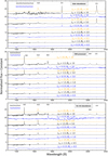 |
Fig. A.1. Ultraviolet spectral region of the CMFGEN models shown Fig. 1. The models have been continuum normalised and shifted. The labels indicate the adopted values of Ṁ3 (10−3 M⊙ yr−1) and L9 (109 L⊙), and the strongest spectral lines are identified. |
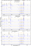 |
Fig. A.3. High-resolution CMFGEN optical spectra of SNe interacting with their progenitor’s wind at early times. The models have been continuum normalised and shifted. The labels indicate the adopted values of Ṁ3 (10−3 M⊙ yr−1) and L9 (109 L⊙), and the strongest spectral lines are identified. |
All Tables
All Figures
|
Fig. 1. CMFGEN optical spectra of SNe interacting with their progenitor’s wind at early times for solar (top panel), CNO-processed (middle panel), and He-rich abundances (bottom panel). The models have been convolved with a Gaussian kernel of Δv = 300 km s−1 (resolving power R ≈ 1000), continuum normalised, and shifted for clarity. The labels indicate the adopted values of Ṁ3 (10−3 M⊙ yr−1) and L9 (109 L⊙), and the strongest spectral lines are identified. |
| In the text | |
|
Fig. 2. CMFGEN optical spectra of SNe interacting with their progenitor’s wind at early times for solar (top panel), CNO-processed (middle panel), and He-rich abundances (bottom panel). The models have been convolved with a Gaussian kernel of Δv = 300 km s−1 (resolving power R ≈ 1000), continuum normalised, and shifted for clarity. All the models in this figure have Ṁ = 3 × 10⁻³ M⊙ yr−1. The labels indicate the adopted values of L9 (109 L⊙), and the strongest spectral lines are identified. |
| In the text | |
|
Fig. 3. CMFGEN optical spectra of SNe interacting with their progenitor’s wind at early times for progenitors with υ∞ = 150 km s−1 (models from Fig. 1; black) and with υ∞ = 15 km s−1 (overplotted on the corresponding high υ∞ models; yellow). The models have been convolved with a Gaussian kernel of Δv = 300 km s−1 (resolving power R ≈ 1000), continuum normalised, and shifted for clarity. The labels indicate the adopted values of Ṁ3 (10−3 M⊙ yr−1), and the strongest spectral lines are identified. All the models in this figure have solar abundances and L = 1.5 × 10⁹ L⊙. |
| In the text | |
|
Fig. 4. Low-resolution (Δv = 1000 km s−1, R ≈ 300) CMFGEN optical spectra of SNe interacting with their progenitor’s wind at early times for solar (top panel), CNO-processed (middle panel), and He-rich abundances (bottom panel). The models have been continuum normalised and shifted for clarity. The labels indicate the adopted values of Ṁ3 (10−3 M⊙ yr−1) and L9 (109 L⊙), and the strongest spectral lines are identified. |
| In the text | |
|
Fig. A.1. Ultraviolet spectral region of the CMFGEN models shown Fig. 1. The models have been continuum normalised and shifted. The labels indicate the adopted values of Ṁ3 (10−3 M⊙ yr−1) and L9 (109 L⊙), and the strongest spectral lines are identified. |
| In the text | |
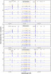 |
Fig. A.2. Similar to Fig. A.1, but for near-infrared spectral region. |
| In the text | |
|
Fig. A.3. High-resolution CMFGEN optical spectra of SNe interacting with their progenitor’s wind at early times. The models have been continuum normalised and shifted. The labels indicate the adopted values of Ṁ3 (10−3 M⊙ yr−1) and L9 (109 L⊙), and the strongest spectral lines are identified. |
| In the text | |
Current usage metrics show cumulative count of Article Views (full-text article views including HTML views, PDF and ePub downloads, according to the available data) and Abstracts Views on Vision4Press platform.
Data correspond to usage on the plateform after 2015. The current usage metrics is available 48-96 hours after online publication and is updated daily on week days.
Initial download of the metrics may take a while.