| Issue |
A&A
Volume 621, January 2019
|
|
|---|---|---|
| Article Number | A89 | |
| Number of page(s) | 10 | |
| Section | Astrophysical processes | |
| DOI | https://doi.org/10.1051/0004-6361/201732383 | |
| Published online | 14 January 2019 | |
A broadband spectral analysis of 4U 1702-429 using XMM-Newton and BeppoSAX data
1
Dipartimento di Fisica e Chimica, Università di Palermo, Via Archirafi 36, 90123 Palermo, Italy
e-mail: This email address is being protected from spambots. You need JavaScript enabled to view it.
2
Dipartimento di Fisica, Università degli Studi di Cagliari, SP Monserrato-Sestu, KM 0.7, Monserrato 09042, Italy
3
Istituto Nazionale di Astrofisica, IASF Palermo, Via U. La Malfa 153, 90146 Palermo, Italy
4
IAAT Universität Tüingen, Sand 1, 72076 Tübingen, Germany
5 INAF-Osservatorio Astronomico di Cagliari, Via della Scienza 5, 09047 Selargius, Italy
Received:
29
November
2017
Accepted:
27
November
2018
Abstract
Context. Most of the X-ray binary systems containing neutron stars classified as Atoll sources show two different spectral states, referred to as soft and hard. Moreover, a large number of these systems show a reflection component relativistically smeared in their spectra, which provides information on the innermost region of the system.
Aims. Our aim is to investigate the poorly studied broadband spectrum of the low-mass X-ray binary system 4U 1702-429, which was recently analysed combining XMM-Newton and INTEGRAL data. The peculiar value of the reflection fraction brought us to analyse further broadband spectra of 4U 1702-429.
Methods. We re-analysed the spectrum of the XMM-Newton/INTEGRAL observation of 4U 1702-429 in the 0.3–60 keV energy range and we extracted three 0.1–100 keV spectra of the source analysing three observations collected with the BeppoSAX satellite.
Results. We find that the XMM-Newton/INTEGRAL spectrum is well fitted using a model composed of a disc blackbody plus a Comptonised component and a smeared reflection component. We used the same spectral model for the BeppoSAX spectra, finding that the addition of a smeared reflection component is statistically significant. The best-fit values of the parameters are compatible to each other for the BeppoSAX spectra. We find that the reflection fraction is 0.05−0.01+0.3 for the XMM-Newton/INTEGRAL spectrum and between 0.15 and 0.4 for the BeppoSAX ones.
Conclusions. The relative reflection fraction and the ionisation parameter are incompatible between the XMM-Newton/INTEGRAL and the BeppoSAX observations and the characteristics of the Comptonising corona suggest that the source was in a soft state in the former observation and in a hard state in the latter.
Key words: stars: neutron / stars: individual: 4U 1702-429 / X-rays: binaries / accretion, accretion disks
© ESO 2019
1. Introduction
Low-mass X-ray binaries hosting neutron stars (NS-LMXBs) are binary systems in which a weakly magnetised neutron star (NS) accretes matter from a low-mass (< 1 M⊙) companion star via the Roche-lobe overflow. In the X-ray spectra of these sources we can distinguish some main components: a soft thermal component due to the blackbody emission from the NS and/or the accretion disc, a hard component due to the Comptonisation of soft photons from a hot electron corona located in the innermost region of the system, and the reflection component originating from the interaction of photons leaving the Comptonising cloud and scattered by the surface of the disc. The emission of a NS-LMXB is characterised by two spectral states, referred to as soft and hard. In the soft state (SS) the continuum spectrum can be described by a (predominant) blackbody or disc-blackbody component and a harder saturated Comptonised component (see e.g. Di Salvo et al. 2009, 2005; Piraino et al. 2007; Barret & Olive 2002). Meanwhile, the hard state (HS) spectrum can be described by a weak thermal emission, sometimes not significantly detected (see e.g. Ludlam et al. 2016), plus a power law with a high-energy cut-off explained as due to inverse Compton scattering of soft photons in the hot electron corona (see e.g. Di Salvo et al. 2015; D’Aì et al. 2010; Cackett et al. 2010). Some HS spectra have been described in terms of a hybrid model of a broken power-law/thermal Comptonisation component plus two blackbody components (Lin et al. 2007; Armas Padilla et al. 2017). The use of a broken power-law model however, does not allow for information to be obtained about the origin of the seed photons of the Comptonised component, that is, it does not allow one to distinguish between the contribution to the Comptonised component of a blackbody or a disc-blackbody. In this sense, a Comptonisation model is more useful for the identification of the origin of all the spectral components, and in particular the main component responsible for the soft thermal emission. Recently, some HS spectra have been interpreted in terms of a double Comptonised component with seed photons emitted by NS and the accretion disc (Zhang et al. 2016).
The broad-band spectral analysis is useful in order to obtain information on the nature of the compact object (a BH or a NS) present in a LMXB, as well as to infer information on the innermost region of the system (e.g. Di Salvo et al. 2006). Of particular interest, in this sense, is the study of the reflection component that originates from direct Compton scattering of the Comptonized photons outgoing the hot corona with the cold electrons in the top layers of the inner accretion disc. In most cases, these studies result in the so-called Compton hump around 20–40 keV (Egron et al. 2013; Miller et al. 2013; Barret et al. 2000). The reflection component can also show some discrete features due to the fluorescence emission and photoelectric absorption by heavy ions in the accretion disc. The reflection is more efficient in SS, usually showing a higher degree of ionisation of the accreting matter (ξ > 500) and the presence of stronger features with respect to HS. This is seen both in NS-LMXBs (Di Salvo et al. 2015; Egron et al. 2013) and in BH-LMXBs (Done et al. 2007). The efficiency of the reflection is mainly indicated by the presence of a strong emission line from highly ionised Fe atoms; this probably reflects the greater emissivity of the accretion disc, which is proportional to r−betor, where r is the radius of the disc at which the incident radiation arrives and betor is the power-law dependence of emissivity and is usually found to be between 2 (in the case of a dominating central illuminating flux) and 3 (which describes approximately the intrinsic emissivity of a disc). The higher emissivity in SS is the consequence of the disc (generally) being closer to the NS surface than in HS. Indeed, broad emission lines (full width at half maximum – FWHM – up to 1 keV) in the Fe-K region (6.4–6.97 keV) are often observed in the spectra of NS-LMXBs with both an inclination angle lower than 60° (e.g. Matranga et al. 2017a; Chiang et al. 2016; Papitto et al. 2013; Sanna et al. 2013; Piraino et al. 2012; Cackett et al. 2008, 2009; Di Salvo et al. 2009; Iaria et al. 2009; Shaposhnikov et al. 2009; Pandel et al. 2008) and with an inclination angle between 60° and 90° (the so-called dipping and eclipsing sources; e.g. Ponti et al. 2018; Pintore et al. 2015; Díaz Trigo et al. 2012, 2009; Iaria et al. 2007; Boirin et al. 2005; Parmar et al. 2002; Sidoli et al. 2001). These broad lines are identified with the Kα radiative transitions of iron at different ionisation states, and most likely originate in the region of the accretion disc close to the compact object where matter is rapidly rotating and reaches velocities up to a few tenths of the speed of light. Hence, the whole reflection spectrum is believed to be modified by Doppler shift, Doppler broadening, and gravitational redshift (see e.g. Fabian et al. 1989; Laor 1991), which produce the characteristic broad and skewed line profile.
It should be mentioned that relativistic (plus Compton) broadening is not the unique physical interpretation for the large width of the iron line profile in these systems. For instance, Titarchuk et al. (2003) suggested that the characteristic asymmetric skewed profile of the iron line could originate from an optically thick flow ejected from the disc, outflowing at relativistic speeds. However, for an increase of the observed broadening this model requires a corresponding increase of the equivalent hydrogen column due to the increased number of scatterings, and this correlation seems to be absent for NS-LMXBs (Cackett & Miller 2013). The study of the line profile therefore provides important information on the ionisation state, geometry, and velocity field of the reprocessing plasma in the inner accretion flow.
In this paper we report on a broad-band spectral analysis of the X-ray source 4U 1702-429 (Ara X-1) that is a NS-LMXB showing type-I X-ray bursts. The source was detected as a burster with OSO 8 (Swank et al. 1976). Oosterbroek et al. (1991) classified 4U 1702-429 as an atoll source using EXOSAT data. Galloway et al. (2008), analysing the photospheric radius expansion of the observed type-I X-ray bursts, inferred a distance to the source of 4.19 ± 0.15 kpc and 5.46 ± 0.19 kpc for a pure hydrogen and pure helium companion star, respectively. Markwardt et al. (1999), using the data of the proportional counter array (PCA) onboard the Rossi X-ray Timing Explorer (RXTE) satellite, detected burst oscillations at 330 Hz that could be associated with the spin frequency of the NS.
Using Einstein data, Christian & Swank (1997) modelled the continuum emission adopting a cut-off power law with a photon index between 1.3 and 1.5 and a cut-off temperature between 8 and 16 keV. Markwardt et al. (1999), analysing RXTE/PCA data, adopted the same model and obtained a temperature between 3.5 and 4.6 keV. Using XMM-Newton and INTEGRAL spectra, Iaria et al. (2016) revealed the presence of a broad emission line at 6.7 keV. These authors fitted the spectra adopting a disc blackbody component plus Comptonisation and reflection component from the accretion disc. An inner disc temperature of 0.34 keV, an electron temperature of 2.3 keV, and a photon index of 1.7 – the latter two associated with the Comptonising cloud – have been obtained. The equivalent hydrogen column density associated with the interstellar medium was 2.5 × 1022 cm−2 and the ionisation parameter associated with the reflecting plasma was logξ = 2.7.
In order to compare recent observations with previous ones and explore different spectral states of the source (in particular, concerning the presence of the reflection component), we re-analysed the XMM-Newton/INTEGRAL spectrum of 4U 1702-429 already studied by Iaria et al. (2016). We also present for the first time the analysis of three 0.1–100 keV BeppoSAX spectra, showing that the addition of a reflection component is statistically required.
2. Observations and data reduction
The narrow field instruments (NFIs) on board the BeppoSAX satellite observed 4U 1702-429 three times between 1999 and 2000. The NFIs are four co-aligned instruments which cover three decades in energy, from 0.1 keV up to 200 keV. The Low-Energy Concentrator Spectrometer (LECS, operating in the range 0.1–10 keV; Parmar et al. 1997) and the Medium-Energy Concentrator Spectrometer (MECS, 1.3–10 keV; Boella et al. 1997) have imaging capabilities with fields of view (FOV) of 20′ and 30′ radii, respectively. We selected data in circular regions – centred on the source – of 8′ and 6′ radii for LECS and MECS, respectively. The background events were extracted from circular regions with the same radii adopted for the source-event extractions and centred in a detector region far from the source. The High-Pressure Gas Scintillator Proportional Counter (HPGSPC, 7–60 keV; Manzo et al. 1997) and Phoswich Detector System (PDS, 13–200 keV; Frontera et al. 1997) are non-imaging instruments, with FOVs of ∼1° FWHM delimited by collimators. The background subtraction for these instruments is obtained using the off-source data accumulated during the rocking of the collimators.
MECS is composed of three modules but only MECS2 and MECS3 were active during these observations. The event files of these two instruments are merged and we indicate them as MECS23. The first observation (obsid. 2069400100, hereafter observation A) was performed between 1999 February 27 17:34:34 UT and February 28 09:12:06 UT for a duration time of 58 ks, the second observation (obsid. 2122400100, hereafter observation B) was performed between 2000 August 24 19:22:51 UT and August 26 01:04:01 UT for a duration time of 104 ks, and finally the third observation (obsid. 2122400200, hereafter observation C) was taken between 2000 September 23 22:41:50 UT and September 25 04:30:29 UT for a duration of 107 ks.
We used several tools of SAXDAS 2.3.3 and HEASOFT 6.20 to extract scientific products from clean event files downloaded from the Multi-Mission Interactive Archive at the ASI Space Science Data Center (SSDC). Initially, we extracted the MECS23 light curve in the 1.3–10 keV energy range for each observation. We show the three MECS light curves with a bin time of 64 s in (Fig. 1). During observation A the count rate is constant at 8.5 c/s from the start time up to 35 ks, when the count rate increases up to 10 c/s (Fig. 1, left panel). During observation B three type-I X-ray bursts are present at 6.6 ks, 43.3 ks, and 92.6 ks from the start time. The count rate at the peak of the bursts is 40 c/s, 35 c/s, and 40 c/s, respectively, whilst the count rate of the persistent emission gradually increases from 9.5 c/s to 11 c/s (Fig. 1, middle panel). During observation C two type-I X-ray bursts are present at 34 ks and 106 ks from the start time. The count rate at the peak of the bursts is 52 c/s and 60 c/s, respectively. The count rate of the persistent emission is constant at 8 c/s (Fig. 1, right panel).
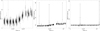 |
Fig. 1. MECS23 light curves of the source 4U 1702-429 for the observations A, B, and C in the left, central, and right panels, respectively. The bin time is 64 s. Three and two type-I X-ray bursts occurred during observations B and C, respectively. |
LECS exposure times are 7.1 ks, 19.4 ks, and 12.3 ks for observation A, B, and C, respectively. LECS light curves corresponding to observations A and C do not show type-I X-ray bursts, while the LECS light curve corresponding to observation B shows only the first type-I X-ray burst observed in the MECS23 light curve of the same observation. The exposure times of each instrument for the three observations are shown in Table 1.
Exposure times of the NFIs for each of the three observations of 4U 1702-429.
Since our aim is the study of the persistent emission of the source, we excluded the bursts detected from the light curves. Using the XSELECT tool, we determined the time intervals at which bursts occurred and excluded them (Table 2). The same operation was carried out on the background light curves to keep the same exposure time.
Time intervals excluded for removing bursts.
Once the time intervals of the bursts were excluded, we build the MECS23 hardness ratio (HR): we divided MECS data in the energy bands 1.6–3 keV and 3–10 keV and produced HR for each observation. We show the 1.6–3 keV light curves, the 3–10 keV light curves, and the corresponding HRs in Fig. 2 for observations A, B, and C. The HRs were relatively constant throughout the observations, and we extracted a spectrum of the persistent emission for each one of them.
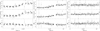 |
Fig. 2. Left panel: MECS23 light curves and HR for observation A. Central panel: MECS23 light curves and HR for observation B. Right panel: MECS23 light curves and HR for observation C. In each panel, from the top to the bottom: MECS23 light curve in the energy band 1.6–3 keV, in the energy band 3–10 keV, and the corresponding hardness ratio. The bin time is 256 s. |
We extracted MECS and LECS spectra using XSELECT, and grouped each one in order to have at least 25 photons for each energy channel. We used the hpproducts and pdproducts tools to obtain the HP and PDS background-subtracted spectra, cleaned of bursts. The PDS spectra were grouped adopting a logarithmic rebinning.
The combined XMM-Newton and INTEGRAL persistent spectrum of 4U 1702-429 used in this work was obtained as described by Iaria et al. (2016). The exposure times are 37 ks for the reflection grating spectrometers (RGS; den Herder et al. 2001), and 36 ks for the spectra collected by the two MOS charge-coupled devices (CCDs; MOS1 and MOS2, Turner et al. 2001) and by the pn CCDs (PN; Strüder et al. 2001) of the European Photon Imaging Camera (EPIC). The MOS1 and MOS2 spectra were combined, as were the RGS1 and RGS2 spectra. The exposure times of JEM-X2 (Lund et al. 2003) and IBIS/ISGRI (Ubertini et al. 2003; Lebrun et al. 2003) were 6 ks and 130 ks, respectively.
3. Spectral analysis
We used the XSPEC software package v12.9.1 to fit the spectra. For all observations we fitted the continuum direct emission with a model composed of a multicolour disc blackbody emission (diskbb in XSPEC, Mitsuda et al. 1984; Makishima et al. 1986) plus a thermal Comptonisation (nthComp in XSPEC, Zdziarski et al. 1996; Życki et al. 1999), in which the inp_type parameter was set to 1, indicating that the seed photons were emitted by the accretion disc; both the components were multiplied by the phabs component, which takes into account the photoelectric absorption by neutral matter in the ISM. We set the abundances to the values found by Wilms et al. (2000) and the photoelectric absorption cross-sections were set to the values obtained by Verner et al. (1996).
Furthermore, in our analysis we assumed a distance to the source of 5.5 kpc (Iaria et al. 2016) and a neutron star mass of 1.4 M⊙.
3.1. Re-analysis of the XMM-Newton/INTEGRAL spectrum
We re-analysed the XMM-Newton/INTEGRAL spectrum using the data in the energy ranges 0.6–2.0 keV for RGS12, 0.3–10 keV for MOS12, 2.4–10 keV for PN, 5–25 keV for JEM-X2, and 20–50 keV for ISGRI.
We initially fitted the XMM-Newton/INTEGRAL data using the same self-consistent model used by Iaria et al. (2016), in which the continuum emission was described as reported above. The inner disc temperature kTbb and the disc-blackbody normalisation were left free to vary, as well as the photon index Γ, the electron temperature kTe, and the seed photon temperature kTseed.
To fit the emission line in the Fe-K region we adopted the self-consistent reflection model rfxconv (Kolehmainen et al. 2011) in which we kept the iron abundance fixed to the solar one and left the ionisation parameter logξ of the reflecting matter in the accretion disc and the reflection fraction rel_refl free to vary. To take into account the relativistic smearing effects in the inner region of the accretion disc, we used the multiplicative rdblur component, in which we kept the outer radius fixed at the value of 1000 gravitational radii (Rg = GM/c2), while leaving the inclination angle θ of the binary system, the inner radius Rin at which the reflection component originates, and the power-law dependence of emissivity betor free to vary. The incident emission onto the accretion disc is provided by the Comptonisation component. We obtained best-fit results consistent with the results reported by Iaria et al. (2016) with a χ2(d.o.f.) of 2578(2247), but we observed large residuals between 3 and 4 keV. To fit these residuals, we added two relativistically broad lines with a fixed energy of 3.32 keV and of 3.9 keV (corresponding to the emission line of Ar XVIII and Ca XIX ions), respectively. We call this model
![Mathematical equation: $$ \begin{aligned}&\mathtt{Model\,1{:}}\;{\mathrm{edge}} *{\mathrm{edge}} *{\mathrm{phabs}} *\{ {\mathrm{diskbb}} + \\&{\mathrm{rdblur}} *({\mathrm{gauss}} + {\mathrm{gauss}} + {\mathrm{rfxconv}} *{\mathrm{nthComp}}[{\mathrm{inp}}\_{\mathrm{type}}=1])\}, \end{aligned} $$](/articles/aa/full_html/2019/01/aa32383-17/aa32383-17-eq2.gif)
and show the best-fit results in the second column of Table 3. From this model we obtained a χ2(d.o.f.) of 2559(2245) and Δχ2 = 19, with an F-test probability of chance improvement of 2.47 × 10⁻⁴ (corresponding to a significance of ∼3.8σ) which suggests that the addition of both the lines is statistically significant. The significances of the two lines associated with Ar XVIII and Ca XIX are ∼4σ and ∼3σ, respectively.
Best-fit values of the spectral models for XMM-Newton data.
We observed a variation in all the parameters of the continuum. In particular, we obtained a value of kTseed larger than kTbb suggesting that the seed photons are not emitted by the accretion disc only but a possible contribution of photons emitted by the neutron star surface is present. For this reason, we fitted the data with
![Mathematical equation: $$ \begin{aligned} \mathtt{Model\,2{:}}\;{\mathrm{phabs}} *\{ {\mathrm{diskbb}} + {\mathrm{nthComp}}[{\mathrm{inp}}\_{\mathrm{type}}=0]\}, \end{aligned} $$](/articles/aa/full_html/2019/01/aa32383-17/aa32383-17-eq34.gif)
in which the inp_type parameter set to 0 indicates seed photons emitted by NS, and we obtained a χ2(d.o.f.) of 2844(2252).
Large residuals remain in the Fe-K region and between 3 and 4 keV; to fit those we added three diskline (Fabian et al. 1989) components for which we kept fixed the energies of two out of three lines at 3.32 and 3.9 keV, while the energy of the third one was left free to vary. For the two lines with fixed energy, we tied the values of inclination angle, power law emissivity dependence, and blackbody radius to those of the third one. The outer radius of the reflecting region was set to 1000 Rg for each line. Finally, we imposed that the inner radius of the reflecting region had the same value of the inner radius of the accretion disc. The best-fit results, obtained by adding the three disc lines, showed a χ2(d.o.f.) of 2640(2246), with an F-test probability of chance improvement of 1.13 × 10⁻³³. Large residuals were still present at 0.8 keV and 8.8 keV, and for this reason we added two absorption edges fixing the energy threshold at 0.871 keV and 8.828 keV, associated with the presence of O VIII and Fe XXVI ions, respectively. We called this model
![Mathematical equation: $$ \begin{aligned}&\mathtt{Model\,3{:}}\;{\mathrm{edge}} *{\mathrm{edge}} *{\mathrm{phabs}} *\{ {\mathrm{diskline}} +\\&{\mathrm{diskline}} + {\mathrm{diskline}} +{\mathrm{diskbb}} + {\mathrm{nthComp}}[{\mathrm{inp}}\_{\mathrm{type}}=0]\}. \end{aligned} $$](/articles/aa/full_html/2019/01/aa32383-17/aa32383-17-eq35.gif)
We obtained a χ2(d.o.f.) of 2523(2244), with an F-test probability of chance improvement of 1 × 10⁻²² (corresponding to a significance much higher than 6σ) and a Δχ2 of 117 with respect to the previous model. We obtained a significance of 19σ, 4σ, and 6σ for the Ar XVIII, Ca XIX, and Fe XXVI emission lines, respectively. The energy of the smeared emission line in the Fe-K region is 6.81 ± 0.07 keV, which is compatible within 3σ with the rest frame value. The best-fit results are shown in the third column of Table 3.
Although Model 3 presented statistically good results, we decided to fit the data using also the self-consistent approach described above, which takes into account the reflection continuum. We kept fixed the outer radius in the rdblur component at the value of 1000 Rg and the power-law dependence of emissivity at the value of −2.5, consistent with the result of Model 3. In this case we imposed that the value of Rin be the same as that of Rdisc. Since the rfxconv model does not account for the emission lines associated to ionised Argon and Calcium, we added two Gaussian components with energies fixed at 3.32 and 3.9 keV, respectively. We call this model
![Mathematical equation: $$ \begin{aligned}&\mathtt{Model\,4{:}}\;{\mathrm{edge}} *{\mathrm{edge}} *{\mathrm{phabs}} *\{ {\mathrm{diskbb}} + \\&{\mathrm{rdblur}} *({\mathrm{gauss}} + {\mathrm{gauss}} + {\mathrm{rfxconv}} *{\mathrm{nthComp}}[{\mathrm{inp}}\_{\mathrm{type}}=0])\}. \end{aligned} $$](/articles/aa/full_html/2019/01/aa32383-17/aa32383-17-eq36.gif)
Using this self-consistent model we obtained a χ2(d.o.f.) of 2550(2245), with a large improvement with respect to Model 2 and a significance of 6σ for both Ar XVIII and Ca XIX emission lines. We show the comparison between the residuals obtained using Model 2 and Model 4 in Fig. 3; the best-fit values of the parameters are shown in the fourth column of Table 3.
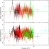 |
Fig. 3. Comparison between residuals obtained adopting Model 2 (top panel) and Model 4 (lower panel). The RGS12, MOS12, PN, JEM-X2, and ISGRI data are shown in black, red, green, blue, and cyan colour, respectively. |
Finally, we find that the total unabsorbed flux is 3.8 × 10⁻⁹ erg cm−2 s−1 in the 0.1–100 keV energy range; the corresponding luminosity is 1.5 × 1037 erg s−1.
3.2. The Beppo SAX spectra
We adopted the 0.12–4 keV, 1.8–10 keV, 7–25 keV, and 15–100 keV energy range for LECS, MECS, HPGSP, and PDS spectra, respectively. Hereafter we refer to the spectra obtained from observations A, B, and C as spectra A, B, and C.
Initially, we fitted the continuum emission with Model 2. Assuming that NH does not change with respect to XMM-Newton/INTEGRAL observations and considering the low statistics of the BeppoSAX/LECS data below 1 keV, we kept the value of equivalent hydrogen column associated with the interstellar matter fixed to 2.42 × 1022 cm−2, as obtained from best-fit values of Model 4 (see Table 3). Fitting the data we obtained a χ2(d.o.f.) of 472(477), 650(502), and 532(481) for spectra A, B, and C, respectively. The best-fit results are shown in the second, third, and fourth columns of Table 4.
Best-fit values of the spectral models for BeppoSAX data.
We observed that some residuals are present in the Fe-K region of the spectra A and C and these are slightly larger for spectrum B. For this reason we added a smeared reflection component to Model 2. We adopted the Compton reflection model described for the analysis of the XMM-Newton/INTEGRAL spectrum. The inclination angle was kept fixed to 38° as obtained from Model 4 (see Table 3). In this case, the inner radius Rin, the ionisation parameter logξ, and the reflection fraction rel_refl were left free to vary. We call this model
![Mathematical equation: $$ \begin{aligned}&\mathtt{Model\,5{:}}\;\mathrm{{phabs}} *\{ \mathrm{{diskbb}} +\\&\mathrm{{rdblur}} * \mathrm{{rfxconv}} * \mathrm{{nthComp}}[\mathrm{{inp}}\_{\rm {type}}=0]\}. \end{aligned} $$](/articles/aa/full_html/2019/01/aa32383-17/aa32383-17-eq48.gif)
For observation B we obtained a χ2(d.o.f.) of 558(499), and found the F-test probability of chance improvement for the addition of the reflection component to be 2.0 × 10⁻¹⁶. The Fe-K region of the spectrum does not show significant residuals anymore. The best-fit values of the parameters are shown in the sixth column of Table 4. The unfolded spectrum and the residuals are shown in the central panels of Figs. 4 and 5, respectively.
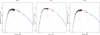 |
Fig. 4. Unfolded spectra of the three BeppoSAX observations fitted adopting Model 5. The LECS, MECS23, HPGSP, and PDS spectra are shown in black, red, green, and blue, respectively. |
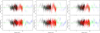 |
Fig. 5. Comparison between residuals obtained adopting Model 2 (top panels) and Model 5 (bottom panels) for observation A (on the left), observation B (in the middle) and observation C (on the right). The black, red, green and blue points represent the LECS, MECS23, HPGSP, and PDS data, respectively. |
Subsequently, we adopted the Model 5 to fit spectra A and C. For spectrum C, we obtained a χ2(d.o.f.) of 482(478) and an F-test probability of chance improvement of 3.1 × 10⁻¹⁰ (significance higher than 6σ). The ionisation parameter logξ and the relative reflection normalisation rel_refl are  and 0.2 ± 0.1, respectively, and they are compatible within 90% c.l. with the values obtained for spectrum B. The best-fit values of the parameters for spectrum C are shown in the seventh column of Fig. 4.
For spectrum A, we needed to fix the value of the ionisation parameter in order to lead the fit to convergence. We chose the best value logξ = 3.14 obtained from the contour plot, shown in Fig. 6. This two-dimensional distribution of the χ2 as a function of the ionisation and the reflection amplitude was obtained varying logξ between 2.1 and 4 and rel_refl between −0.6 and −0.01 simultaneously through the steppar tool in XSPEC. Moreover, the inner radius of the reflection region was kept fixed to the value of 24 km because the χ2 was insensitive to the variation of this parameter. The value of 24 km was obtained from Model 5 leaving Rin free to vary and keeping all the other parameters fixed. We obtained a χ2(d.o.f.) of 449(476) and the F-test gives a probability of chance improvement of 1.1 × 10⁻⁶, corresponding to a significance of ∼4.9σ.
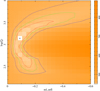 |
Fig. 6. Contour plot of χ2 changes for simultaneous variation of logξ and rel_refl parameters for spectrum A. The red, green; and blue lines indicate the contours at 68, 90, and 99% confidence level, respectively. The black cross indicates the best-fit values of logξ = 3.14 and rel_refl = 0.1. The orange-scale indicates the value of χ2 changes in the grid. |
The best-fit values of the parameters for spectrum A are shown in the fifth column of Table 4. The unfolded spectrum and the residuals are shown in the left and right panels of Figs. 4 and 5 for spectra A and C, respectively.
We found a total unabsorbed flux of 1.5 × 10⁻⁹ erg cm−2 s−1 for spectrum A, 2.1 × 10⁻⁹ erg cm−2 s−1 for spectrum B, and 1.3 × 10⁻⁹ erg cm−2 s−1 for spectrum C. Finally, the corresponding luminosities are 5.5 × 1036 erg s−1, 7.5 × 1036 erg s−1, and 4.8 × 1036 erg s−1, respectively.
4. Discussion
We re-analysed the observations of the NS-LMXB 4U 1702-429 taken with XMM-Newton/INTEGRAL in March 2010 and we analysed three BeppoSAX observations performed in February 1999, August 2000 and September 2000. The broadband analysis indicates that the addition of a smeared reflection component to the spectral model is statistically significant in the case of the XMM-Newton/INTEGRAL observation and observations B and C, and is marginally significant for observation A.
The smeared reflection component allowed us to constrain the inclination angle θ of the source, which is  deg. using the XMM-Newton/INTEGRAL spectrum.
The 0.1–100 keV unabsorbed luminosity is a factor of two to three larger during the XMM-Newton/INTEGRAL observation than that obtained from the three BeppoSAX observations (see previous section). Moreover, the electron temperature is  for the XMM-Newton/INTEGRAL spectrum while it is
  ,
,  , and
, and  for spectra A, B, and C, respectively. This suggests that the source was in a SS during the XMM-Newton/INTEGRAL observation and in a HS during the three BeppoSAX observations.
From Model 4 we obtain  for XMM-Newton/INTEGRAL spectrum, while Rdisc is
  , 12 ± 1 km, and 14 ± 3 km for spectra A, B, and C, respectively, adopting Model 5. We applied the correction factor to convert the inner radius Rdisc values into the realistic inner radius rdisc values. The relation between these two radii is rdisc ∼ f2Rdisc, where the colour correction factor f ≃ 1.7 for a luminosity close to 10% of Eddington luminosity (Shimura & Takahara 1995). We find that the rdisc values are
  ,
,  , 35 ± 3 km, and 40 ± 9 km for the XMM-Newton/INTEGRAL observation and for spectra A, B, and C, respectively. The rdisc values are compatible with each other within 90% c.l. for the three BeppoSAX spectra, while the value obtained from the XMM-Newton/INTEGRAL spectrum is larger by a factor of about two. We note that the behaviour of the disc blackbody radius is similar to that obtained by Di Salvo et al. (2015) for the prototype atoll source 4U 1705-44. In that case the authors observed an inner radius of the blackbody component close to 11 km in the HS and about 33 km in the SS. Furthermore, the obtained values of rdisc also seem to suggest that the spectrum of 4U 1702-429 is in a SS during the XMM-Newton/INTEGRAL observation, while it is in a HS during the three BeppoSAX observations.
This result could be explained assuming that the inner region of the accretion disc is occulted by an optically thick corona during the XMM-Newton/INTEGRAL observation. To verify the proposed scenario we estimated the optical depth τ of the Comptonising cloud using the relation provided by Zdziarski et al. (1996):
![Mathematical equation: $$ \begin{aligned} \Gamma = \left[\dfrac{9}{4} + \dfrac{1}{\tau \left(1+ \frac{\tau }{3} \right) \frac{kT_{\rm e}}{m_{\rm e}c^2}} \right]^ {1/2} - \dfrac{1}{2}\cdot \end{aligned} $$](/articles/aa/full_html/2019/01/aa32383-17/aa32383-17-eq59.gif)
We found that  during the XMM-Newton/INTEGRAL observation while
  ,
,  , and
, and  for spectra A, B, and C, respectively. Our results suggest that the corona is optically thick during the XMM-Newton/INTEGRAL observation, while the optical depth is much lower during the BeppoSAX observations. The obtained values of τ support the idea that the innermost region of the system is embedded in an optically thick corona in the SS, while the optically thin corona observed in the spectra A, B, and C allows us to look through at the innermost region.
Since the inner radius is between 30 and 50 km (for spectra A, B, and C) we might suppose that the accretion disc is truncated and does not reach the NS surface. This hypothesis is endorsed by the general idea that in a HS the accretion disc is truncated and, in the region near the NS, the hot inner corona can be identified with the boundary layer, whose interactions with the colder accretion disc cause the emptying of the innermost region (Różańska & Czerny 2000). Then the flow and the boundary layer become optically thinner and the thermal emission can be dominated by the neutron star, as suggested by the smallest value of the inner radius of the accretion disc obtained in HS (Barret & Olive 2002).
The two observed spectral states are identified by changes in the electron corona. We note that for the XMM-Newton/INTEGRAL spectrum the electron temperature kTe is about ten times smaller. Since τ ∝ NeR, where R is the size of the Comptonising region, an increase in the optical depth (τ is ten times larger during the XMM-Newton/INTEGRAL observation) can be associated with an increase in the electron density Ne of the corona. Therefore, an increase in the electron density entails an increase in the number of the electrons in the cloud, which is consistent with the observed increase in the flux associated with Comptonised component.
Assuming that the matter almost totally ionised in the accretion disc, we also estimated the electron density ne of the reflecting skin using the relation ξ = LX/(ner2), where LX is the unabsorbed incident luminosity between 0.1 and 100 keV, ξ is the ionisation parameter, and r is the inner radius of the disc where the reflection component originates. We find that for the XMM-Newton/INTEGRAL spectrum  cm−3; on the other hand, since we found only an upper limit for the reflecting radius for BeppoSAX observations, we obtain only a lower limit for the electron density: it is 1.7 × 1021 cm−3 for spectrum A, 1.6 × 1021 cm−3 for spectrum B, and 0.6 × 1021 cm−3 for spectrum C. Therefore, we estimated the seed-photon radius Rseed using the relation Rseed = 3 × 10⁴d[FCompt/(1 + y)]1/2(kTseed)−2 (in ’t Zand et al. 1999), where d is the distance to the source in units of kpc, y = 4kTe max[τ, τ2]/(mec2) is the Compton parameter, kTseed is the seed-photon temperature in units of keV, and FCompt is the bolometric flux of the Comptonisation component. Using the best-fit values (reported in Tables 3 and 4), we find that Rseed is 8 ± 2 km from the XMM-Newton/INTEGRAL spectrum, and it is
  ,
,  , and 10 ± 2 km from the BeppoSAX spectra A, B, and C, respectively. Although we cannot exclude that seed photons originate in the inner accretion disc, this suggests that during observations C and XMM/INTEGRAL the seed photons were mainly emitted from the NS surface, while the smallest values obtained from spectra A and B can be explained assuming that only an equatorial region of the NS surface injects photons in the electron corona.
Typical values of the reflection amplitude Ω/2π for NS-LMXB atoll sources are within 0.2–0.3 (Matranga et al. 2017b; Di Salvo et al. 2015; Egron et al. 2013; D’Aì et al. 2010). However, smaller reflection fractions are also observed for other systems, such as Ser X-1 (Matranga et al. 2017a; Cackett et al. 2010) and 4U 1820-30 (Cackett et al. 2010) and for AMSP SAX J1748.9-2021 (Pintore et al. 2016). We found typical values of Ω/2π for BeppoSAX observations B and C (0.4 ± 0.1 and 0.2 ± 0.1, respectively), whilst we obtained a reflection fraction of  for XMM-Newton/INTEGRAL spectrum, which agrees with the value obtained by Iaria et al. (2016). Since this parameter is a measure of the solid angle subtended by the reflector as seen from the Comptonising corona, our results suggest a slightly different geometry of the electron cloud between SS and HS. In particular, the value obtained for XMM-Newton/INTEGRAL observation could indicate a small subtended angle due, for instance, to a less efficient interaction between the corona and the accretion disc or a different geometry of the cloud with respect to a central spherical corona contiguous to an outer accretion disc (which is a typical representation). Finally, we found that rel_refl = 0.09 ± 0.04 for spectrum A, which is compatible with the value obtained for spectrum C, although the reflection component is unconstrained in this case and this does not represent a conclusive result.
In the case of this source the variation in the spectral state is likely caused by the changes occurring in the Comptonising corona, as suggested by Barret & Olive (2002) for 4U 1705-44. Indeed, the spectral component whose parameters show significant variation between the XMM-Newton/INTEGRAL analysis and the BeppoSAX analysis is the Comptonisation (see Tables 3 and 4).
In conclusion, we do not observe emission lines and absorption edges in the BeppoSAX spectra like those detected in the XMM-Newton/INTEGRAL spectrum because of the smaller effective area and poorer energy resolution of BeppoSAX/MECS with respect to the XMM/EPIC-PN.
4.1. BH-systems comparison
Binary systems hosting a neutron star show similar spectral characteristics with respect to black hole systems, and it would be very hard to distinguish between these two kinds of systems looking only at their spectra. In the BH-candidate systems the accreting matter may free fall into the compact object because close to the event horizon the gravitational force predominates the pressure forces. On the other hand, in the NS systems, the free fall of accreting matter is slowed down by the presence of the solid surface emitting a large part of the total flux and therefore radiation pressure forces should be predominant. Generally this means a mass accretion rate higher than for a NS system and possibly a hotter Comptonized component (Di Salvo et al. 2006).
In BH systems a correlation seems to be present between the softness (or hardness) of the spectrum and the value of the photon index; in particular, the steeper the power law, the softer the spectrum (Steiner et al. 2016). For NS systems this correlation does not always seem to be present: for example, in the case of 4U 1702-429, for the BeppoSAX data the photon index is higher than for the XMM-Newton/INTEGRAL spectrum, although the BeppoSAX spectra are harder than this one. Furthermore, as for BH systems the spectral variation is led by the variation in the flux of the seed photons in the corona and then in a variation in the flux of the outgoing Comptonised photons (Del Santo et al. 2008).
The emission lines observed in the spectra of NS systems turn out to be broadened and skewed like the lines detected in BH-system spectra, suggesting that in both the cases they are produced in the innermost region of the accretion disc, where the effects of the gravitational field of the compact object is stronger. However, both in HS and SS of NS systems, the broadening of the line is not as extreme as in the case of some black-hole X-ray binaries or AGNs (see e.g. Reis et al. 2009; Fabian et al. 2009).
The reflection component has a similar behaviour in BH and NS systems and turns out to be more evident in the SS than in the HS, at least in the standard X-ray range (2–10 keV), with the presence of stronger features (see e.g. Di Salvo et al. 2009, 2015; Egron et al. 2013 for NS systems and Steiner et al. 2016; Zdziarski 2002 for BH systems). In the case of the source 4U 1702-429 the comparison of the reflection features between SS and HS is difficult because of the low statistics at higher energy for BeppoSAX data, which do not allow us to observe the same emission lines observed in the XMM-Newton/INTEGRAL spectrum. We obtained incompatible values for the reflection fraction and the ionisation parameter, which suggests that the geometry of the system and the physical characteristics of the electron corona display a variation between the two observed spectral states.
5. Conclusions
We have performed a detailed broadband spectral analysis of the source 4U 1702-429 in the 0.3–60 keV energy range using an XMM-Newton/INTEGRAL observation and studying separately the data of three observations collected by BeppoSAX in the 0.1–100 keV energy range. Using a self-consistent reflection model, the main results of our analysis are the following:
-
The reflection fraction and the ionisation parameter of the reflection component are incompatible between the XMM-Newton/INTEGRAL spectrum and the BeppoSAX observations. Moreover, we observe an optically thin electron cloud with an electron temperature larger than 30 keV in the BeppoSAX spectra and a colder (∼3 keV) optically thick corona in the XMM-Newton/INTEGRAL spectrum. Furthermore, we find that the total unabsorbed bolometric flux is only twice larger in the case of the XMM-Newton/INTEGRAL observation with respect to BeppoSAX observations.
-
In the XMM-Newton/INTEGRAL spectrum we detect the presence of three emission lines due to the fluorescence emission from Ar XVIII, Ca XIX, and Fe XXV, and two absorption edges identified as the presence of O VIII and Fe XXVI in the accretion disc.
-
For the BeppoSAX observations the best-fit parameters describe a physical scenario of a source in a HS, whilst the XMM-Newton/INTEGRAL spectrum could be associated with a SS.
-
The inner radius of the accretion disc seems to be smaller in the HS (i.e. the disc is closer to the NS surface). This is probably due to the presence of an optically thinner corona than in SS, which allows us to observe the emission from the innermost region of the system. In particular, we might observe a higher contribution from the boundary layer near the NS surface, which is shielded instead from the optically thick corona during SS. This suggests that in SS the thermal component is probably well-fitted by a disc multicolour blackbody, while in HS two blackbody components might be a better description of the soft component: the first one to describe the accretion disc emission and the second one for the boundary layer emission (see e.g. Armas Padilla et al. 2017).
Further broadband observations are needed to confirm our scenario.
Acknowledgments
Part of this work is based on archival data and software provided by the Space Science Data Center – ASI. This research has made use of data and/or software provided by the High Energy Astrophysics Science Archive Research Center (HEASARC), which is a service of the Astrophysics Science Division at NASA/GSFC and the High Energy Astrophysics Division of the Smithsonian Astrophysical Observatory. The authors acknowledge financial contribution from the agreement ASI-INAF n. 2017-14-H.0. and from the agreement ASI- INAF I/037/12/0 and the support from the HERMES Project, financed by the Italian Space Agency (ASI) Agreement n. 2016/13 U.O. Part of this work has been funded using resources from the research grant “iPeska” (PI: Andrea Possenti) funded under the INAF national call Prin-SKA/CTA approved with the Presidential Decree 70/2016. S.M.M. thanks the research project “Stelle di neutroni come laboratorio di Fisica della Materia Ultradensa: uno studio multifrequenza” financed by Regione Autonoma della Sardegna (scientific project manager prof. Luciano Burderi) in which part of this work was developed. The authors thank Dr. Milvia Capalbi for her kind scientific and technical support. The authors would like to thank the anonymous referee for his/her helpful comments.
References
- Armas Padilla, M., Ueda, Y., Hori, T., Shidatsu, M., & Muñoz-Darias, T. 2017, MNRAS, 467, 290 [NASA ADS] [Google Scholar]
- Barret, D., & Olive, J.-F. 2002, ApJ, 576, 391 [NASA ADS] [CrossRef] [Google Scholar]
- Barret, D., Olive, J. F., Boirin, L., et al. 2000, ApJ, 533, 329 [NASA ADS] [CrossRef] [Google Scholar]
- Boella, G., Butler, R. C., Perola, G. C., et al. 1997, A&AS, 122, 299 [NASA ADS] [CrossRef] [EDP Sciences] [Google Scholar]
- Boirin, L., Méndez, M., Díaz Trigo, M., Parmar, A. N., & Kaastra, J. S. 2005, A&A, 436, 195 [NASA ADS] [CrossRef] [EDP Sciences] [Google Scholar]
- Cackett, E. M., & Miller, J. M. 2013, ApJ, 777, 47 [NASA ADS] [CrossRef] [Google Scholar]
- Cackett, E. M., Miller, J. M., Bhattacharyya, S., et al. 2008, ApJ, 674, 415 [NASA ADS] [CrossRef] [Google Scholar]
- Cackett, E. M., Altamirano, D., Patruno, A., et al. 2009, ApJ, 694, L21 [NASA ADS] [CrossRef] [Google Scholar]
- Cackett, E. M., Miller, J. M., Ballantyne, D. R., et al. 2010, ApJ, 720, 205 [NASA ADS] [CrossRef] [Google Scholar]
- Chiang, C.-Y., Cackett, E. M., Miller, J. M., et al. 2016, ApJ, 821, 105 [NASA ADS] [CrossRef] [Google Scholar]
- Christian, D. J., & Swank, J. H. 1997, ApJS, 109, 177 [NASA ADS] [CrossRef] [Google Scholar]
- D’Aì, A., di Salvo, T., Ballantyne, D., et al. 2010, A&A, 516, A36 [NASA ADS] [CrossRef] [EDP Sciences] [Google Scholar]
- Del Santo, M., Malzac, J., Jourdain, E., Belloni, T., & Ubertini, P. 2008, MNRAS, 390, 227 [NASA ADS] [CrossRef] [Google Scholar]
- den Herder, J. W., Brinkman, A. C., Kahn, S. M., et al. 2001, A&A, 365, L7 [NASA ADS] [CrossRef] [EDP Sciences] [Google Scholar]
- Díaz Trigo, M., Parmar, A. N., Boirin, L., et al. 2009, A&A, 493, 145 [NASA ADS] [CrossRef] [EDP Sciences] [Google Scholar]
- Díaz Trigo, M., Sidoli, L., Boirin, L., & Parmar, A. N. 2012, A&A, 543, A50 [NASA ADS] [CrossRef] [EDP Sciences] [Google Scholar]
- Di Salvo, T., Iaria, R., Méndez, M., et al. 2005, ApJ, 623, L121 [NASA ADS] [CrossRef] [Google Scholar]
- Di Salvo, T., Iaria, R., Robba, N., & Burderi, L. 2006, Chin. J. Astron. Astrophys. Suppl., 6, 183 [Google Scholar]
- Di Salvo, T., D’Aí, A., Iaria, R., et al. 2009, MNRAS, 398, 2022 [NASA ADS] [CrossRef] [Google Scholar]
- Di Salvo, T., Iaria, R., Matranga, M., et al. 2015, MNRAS, 449, 2794 [NASA ADS] [CrossRef] [Google Scholar]
- Done, C., Gierliński, M., & Kubota, A. 2007, A&ARv, 15, 1 [NASA ADS] [CrossRef] [EDP Sciences] [Google Scholar]
- Egron, E., Di Salvo, T., Motta, S., et al. 2013, A&A, 550, A5 [NASA ADS] [CrossRef] [EDP Sciences] [Google Scholar]
- Fabian, A. C., Rees, M. J., Stella, L., & White, N. E. 1989, MNRAS, 238, 729 [NASA ADS] [CrossRef] [Google Scholar]
- Fabian, A. C., Zoghbi, A., Ross, R. R., et al. 2009, Nature, 459, 540 [NASA ADS] [CrossRef] [PubMed] [Google Scholar]
- Frontera, F., Costa, E., dal Fiume, D., et al. 1997, A&AS, 122, 357 [NASA ADS] [CrossRef] [EDP Sciences] [Google Scholar]
- Galloway, D. K., Muno, M. P., Hartman, J. M., Psaltis, D., & Chakrabarty, D. 2008, ApJS, 179, 360 [NASA ADS] [CrossRef] [Google Scholar]
- Iaria, R., Lavagetto, G., D’Aí, A., di Salvo, T., & Robba, N. R. 2007, A&A, 463, 289 [NASA ADS] [CrossRef] [EDP Sciences] [Google Scholar]
- Iaria, R., D’Aí, A., di Salvo, T., et al. 2009, A&A, 505, 1143 [NASA ADS] [CrossRef] [EDP Sciences] [Google Scholar]
- Iaria, R., Di Salvo, T., Del Santo, M., et al. 2016, A&A, 596, A21 [NASA ADS] [CrossRef] [EDP Sciences] [Google Scholar]
- in ’t Zand, J. J. M., Verbunt, F., Strohmayer, T. E., et al. 1999, A&A, 345, 100 [NASA ADS] [Google Scholar]
- Kolehmainen, M., Done, C., & Díaz Trigo, M. 2011, MNRAS, 416, 311 [NASA ADS] [Google Scholar]
- Laor, A. 1991, ApJ, 376, 90 [NASA ADS] [CrossRef] [Google Scholar]
- Lebrun, F., Leray, J. P., Lavocat, P., et al. 2003, A&A, 411, L141 [NASA ADS] [CrossRef] [EDP Sciences] [Google Scholar]
- Lin, D., Remillard, R. A., & Homan, J. 2007, ApJ, 667, 1073 [NASA ADS] [CrossRef] [Google Scholar]
- Ludlam, R., Miller, J. M., Cackett, E., et al. 2016, AAS/Energy Astrophys. Div., 15, 120.14 [NASA ADS] [Google Scholar]
- Lund, N., Budtz-Jørgensen, C., Westergaard, N. J., et al. 2003, A&A, 411, L231 [NASA ADS] [CrossRef] [EDP Sciences] [Google Scholar]
- Makishima, K., Maejima, Y., Mitsuda, K., et al. 1986, ApJ, 308, 635 [NASA ADS] [CrossRef] [Google Scholar]
- Manzo, G., Giarrusso, S., Santangelo, A., et al. 1997, A&AS, 122, 341 [NASA ADS] [CrossRef] [EDP Sciences] [Google Scholar]
- Markwardt, C. B., Strohmayer, T. E., & Swank, J. H. 1999, ApJ, 512, L125 [NASA ADS] [CrossRef] [Google Scholar]
- Matranga, M., Di Salvo, T., Iaria, R., et al. 2017a, A&A, 600, A24 [NASA ADS] [CrossRef] [EDP Sciences] [Google Scholar]
- Matranga, M., Papitto, A., Di Salvo, T., et al. 2017b, A&A, 603, A39 [NASA ADS] [CrossRef] [EDP Sciences] [Google Scholar]
- Miller, J. M., Parker, M. L., Fuerst, F., et al. 2013, ApJ, 779, L2 [NASA ADS] [CrossRef] [Google Scholar]
- Mitsuda, K., Inoue, H., Koyama, K., et al. 1984, PASJ, 36, 741 [NASA ADS] [Google Scholar]
- Oosterbroek, T., Penninx, W., van der Klis, M., van Paradijs, J., & Lewin, W. H. G. 1991, A&A, 250, 389 [NASA ADS] [Google Scholar]
- Pandel, D., Kaaret, P., & Corbel, S. 2008, ApJ, 688, 1288 [NASA ADS] [CrossRef] [Google Scholar]
- Papitto, A., D’Aì, A., Di Salvo, T., et al. 2013, MNRAS, 429, 3411 [NASA ADS] [CrossRef] [Google Scholar]
- Parmar, A. N., Martin, D. D. E., Bavdaz, M., et al. 1997, A&AS, 122, 309 [NASA ADS] [CrossRef] [EDP Sciences] [Google Scholar]
- Parmar, A. N., Oosterbroek, T., Boirin, L., & Lumb, D. 2002, A&A, 386, 910 [NASA ADS] [CrossRef] [EDP Sciences] [Google Scholar]
- Pintore, F., Di Salvo, T., Bozzo, E., et al. 2015, MNRAS, 450, 2016 [NASA ADS] [CrossRef] [Google Scholar]
- Pintore, F., Sanna, A., Di Salvo, T., et al. 2016, MNRAS, 457, 2988 [NASA ADS] [CrossRef] [Google Scholar]
- Piraino, S., Santangelo, A., di Salvo, T., et al. 2007, A&A, 471, L17 [NASA ADS] [CrossRef] [EDP Sciences] [Google Scholar]
- Piraino, S., Santangelo, A., Kaaret, P., et al. 2012, A&A, 542, L27 [NASA ADS] [CrossRef] [EDP Sciences] [Google Scholar]
- Ponti, G., Bianchi, S., Muñoz-Darias, T., et al. 2018, MNRAS, 473, 2304 [NASA ADS] [CrossRef] [Google Scholar]
- Reis, R. C., Fabian, A. C., & Young, A. J. 2009, MNRAS, 399, L1 [NASA ADS] [CrossRef] [Google Scholar]
- Różańska, A., & Czerny, B. 2000, MNRAS, 316, 473 [NASA ADS] [CrossRef] [Google Scholar]
- Sanna, A., Hiemstra, B., Méndez, M., et al. 2013, MNRAS, 432, 1144 [NASA ADS] [CrossRef] [Google Scholar]
- Shaposhnikov, N., Titarchuk, L., & Laurent, P. 2009, ApJ, 699, 1223 [NASA ADS] [CrossRef] [Google Scholar]
- Shimura, T., & Takahara, F. 1995, ApJ, 445, 780 [NASA ADS] [CrossRef] [Google Scholar]
- Sidoli, L., Oosterbroek, T., Parmar, A. N., Lumb, D., & Erd, C. 2001, A&A, 379, 540 [NASA ADS] [CrossRef] [EDP Sciences] [Google Scholar]
- Steiner, J. F., Remillard, R. A., García, J. A., & McClintock, J. E. 2016, ApJ, 829, L22 [NASA ADS] [CrossRef] [Google Scholar]
- Strüder, L., Briel, U., Dennerl, K., et al. 2001, A&A, 365, L18 [NASA ADS] [CrossRef] [EDP Sciences] [Google Scholar]
- Swank, J. H., Becker, R. H., Pravdo, S. H., Saba, J. R., & Serlemitsos, P. J. 1976, IAU Circ., 3010 [Google Scholar]
- Titarchuk, L., Kazanas, D., & Becker, P. A. 2003, ApJ, 598, 411 [NASA ADS] [CrossRef] [Google Scholar]
- Turner, M. J. L., Abbey, A., Arnaud, M., et al. 2001, A&A, 365, L27 [NASA ADS] [CrossRef] [EDP Sciences] [Google Scholar]
- Ubertini, P., Lebrun, F., Di Cocco, G., et al. 2003, A&A, 411, L131 [NASA ADS] [CrossRef] [EDP Sciences] [Google Scholar]
- Verner, D. A., Ferland, G. J., Korista, K. T., & Yakovlev, D. G. 1996, ApJ, 465, 487 [NASA ADS] [CrossRef] [Google Scholar]
- Wilms, J., Allen, A., & McCray, R. 2000, ApJ, 542, 914 [NASA ADS] [CrossRef] [Google Scholar]
- Zdziarski, A. 2002, X-ray Binaries in the Chandra and XMM-Newton Era (with an Emphasis on Targets of Opportunity), 54 [Google Scholar]
- Zdziarski, A. A., Johnson, W. N., & Magdziarz, P. 1996, MNRAS, 283, 193 [NASA ADS] [CrossRef] [Google Scholar]
- Zhang, Z., Sakurai, S., Makishima, K., et al. 2016, ApJ, 823, 131 [NASA ADS] [CrossRef] [Google Scholar]
- Życki, P. T., Done, C., & Smith, D. A. 1999, MNRAS, 309, 561 [NASA ADS] [CrossRef] [Google Scholar]
All Tables
All Figures
|
Fig. 1. MECS23 light curves of the source 4U 1702-429 for the observations A, B, and C in the left, central, and right panels, respectively. The bin time is 64 s. Three and two type-I X-ray bursts occurred during observations B and C, respectively. |
| In the text | |
|
Fig. 2. Left panel: MECS23 light curves and HR for observation A. Central panel: MECS23 light curves and HR for observation B. Right panel: MECS23 light curves and HR for observation C. In each panel, from the top to the bottom: MECS23 light curve in the energy band 1.6–3 keV, in the energy band 3–10 keV, and the corresponding hardness ratio. The bin time is 256 s. |
| In the text | |
|
Fig. 3. Comparison between residuals obtained adopting Model 2 (top panel) and Model 4 (lower panel). The RGS12, MOS12, PN, JEM-X2, and ISGRI data are shown in black, red, green, blue, and cyan colour, respectively. |
| In the text | |
|
Fig. 4. Unfolded spectra of the three BeppoSAX observations fitted adopting Model 5. The LECS, MECS23, HPGSP, and PDS spectra are shown in black, red, green, and blue, respectively. |
| In the text | |
|
Fig. 5. Comparison between residuals obtained adopting Model 2 (top panels) and Model 5 (bottom panels) for observation A (on the left), observation B (in the middle) and observation C (on the right). The black, red, green and blue points represent the LECS, MECS23, HPGSP, and PDS data, respectively. |
| In the text | |
|
Fig. 6. Contour plot of χ2 changes for simultaneous variation of logξ and rel_refl parameters for spectrum A. The red, green; and blue lines indicate the contours at 68, 90, and 99% confidence level, respectively. The black cross indicates the best-fit values of logξ = 3.14 and rel_refl = 0.1. The orange-scale indicates the value of χ2 changes in the grid. |
| In the text | |
Current usage metrics show cumulative count of Article Views (full-text article views including HTML views, PDF and ePub downloads, according to the available data) and Abstracts Views on Vision4Press platform.
Data correspond to usage on the plateform after 2015. The current usage metrics is available 48-96 hours after online publication and is updated daily on week days.
Initial download of the metrics may take a while.