| Issue |
A&A
Volume 620, December 2018
|
|
|---|---|---|
| Article Number | A160 | |
| Number of page(s) | 6 | |
| Section | Celestial mechanics and astrometry | |
| DOI | https://doi.org/10.1051/0004-6361/201834118 | |
| Published online | 11 December 2018 | |
Determining the accuracy of VLBI radio source catalogs
1
School of Astronomy and Space Science, Key Laboratory of Modern Astronomy and Astrophysics (Ministry of Education), Nanjing University, 163 Xianlin Avenue, 210023 Nanjing, PR China
e-mail: liuniu@smail.nju.edu.cn
2
SYRTE, Observatoire de Paris, Université PSL, CNRS, Sorbonne Université, LNE, Paris, France
e-mail: sebastien.lambert@obspm.fr
Received:
22
August
2018
Accepted:
10
October
2018
Aims. We propose to estimate the accuracy of current very long baseline interferometry (VLBI) catalogs.
Methods. The difference of source position estimated from two decimation solutions was analyzed to estimate the scale factor and noise floor for the formal error of radio source positions by two different methods. In one method, we investigated the weighted root-square-mean (wrms) scatter of source positional differences versus the number of observed sessions; for the other one, we compared the wrms difference versus the formal error. Based on the estimated noise floor and scale factor, we determined the realistic error of radio source positions in the standard solution and compared it with that of Gaia DR2 and ICRF2 catalogs.
Results. The estimated scale factors from two methods are rather consistent, which is of ∼1.3 in both coordinates. As for the noise floor, it is estimated to be 20–25 μas for sources observed in at least ten sessions, and it could reduce down to ∼10 μas for sources which have been observed more than 1000 times. The inflated median formal error of our solution is of the same order as the Gaia DR2 catalog in declination and the direction of major axis of the error ellipse, but smaller by a factor of two in right ascension. With respect to the ICRF2 catalog, our solution yields an improved accuracy by a factor of about three.
Conclusions. Currently, the VLBI radio source catalog still provides source positions with the best accuracy which is about 20–25 μas. Moreover, the noise floor of VLBI catalogs could potentially reach 10 μas with more observations in the future.
Key words: astrometry / reference systems / catalogs
© ESO 2018
1. Introduction
Geodetic very long baseline interferometry (VLBI) measures positions of thousands of radio sources (quasars) since 1979.0. Thanks to its unreachable accuracy, the International Astronomical Union (IAU) adopted the International Celestial Reference Frame (ICRF) realized by VLBI to serve as the fundamental celestial reference frame (CRF) in 1998. The current version of ICRF is the second realization of the International Celestial Reference Frame (ICRF2) released in 2009. Fey et al. (2015) determined a noise floor (best positional accuracy) of the ICRF2 to be of 40 micro-arc second (μas) and mentioned that the stability of the ICRF axes is close to 10 μas.
The arrival of the Gaia Celestial Reference Frame (Gaia-CRF2; Gaia Collaboration 2016, 2018b) provides an independent CRF realization with a similar high accuracy to VLBI. The comparison in Gaia Collaboration (2018b) showed that the positional formal error for the ICRF3-prototype subset of the second data release of Gaia mission (Gaia DR2; Gaia Collaboration 2018a) is very close to but still worse than that of the prototype version of ICRF3 – the best VLBI solution at that time. However, several studies, for example, Ryan et al. (1993), and Herring et al. (2002), showed that the formal errors of VLBI products are generally too small and therefore should be scaled up. To represent the realistic error ξ, the usual way is to apply a scale factor s and then add a noise floor f in quadrature to the formal error σ, so that we can recalculate the inflated error as
After inflating the formal error, it is interesting to investigate whether the realistic error of VLBI positions for radio sources could still be better than that of the Gaia DR2. To answer this question, we need to determine the realistic accuracy of current VLBI radio source catalogs by estimating the noise floor and scale factor.
Determining the realistic errors is an important part of the compilation works for ICRF catalogs. For the first generation of ICRF (ICRF1), the realistic error of the radio source position was determined through intercomparison of several VLBI catalogs obtained with various analysis strategies and modeling options. After a series of tests, the scale factor and noise floor were estimated to be 1.5 and 250 μas, respectively (Ma et al. 1998). For ICRF2, the scale factor remained the same but noise floor reduced down to 40 μas, showing a large improvement in VLBI technique from ICRF1 (Fey et al. 2015). Several works concerning the internal accuracy of the VLBI catalogs have been published since the ICRF2 was released. Lambert (2014) checks the offsets of several VLBI astrometric radio catalogs with respect to the ICRF2 catalog and concluded that these radio catalogs showed no significant improvement compared to the ICRF2. Gordon et al. (2016) shows that the re-observation of the so-called VCS sources (VCS-II) reduced down the average positional uncertainties for the re-observed VCS sources by nearly a factor of five. These new observations lead to most of recent astrometric improvements with respect to the ICRF2 and hence possibly contribute significantly to reducing the noise floor of the next generation of ICRF (ICRF3; Gordon 2017). More recently, Frouard et al. (2018) compares a new VLBI solution made at the United States Naval Observatory with the ICRF2 catalog. The authors inflate the formal errors of source positions in their solution by the same way as done in the ICRF2 and find that the inflated median formal errors are smaller by ∼20%–25% compared to the ICRF2. At the 30th IAU General Assembly in August 2018, the new version of ICRF–ICRF3, consisted of radio source positions measured at the three bands (S/X, K, and X/Ka), was adopted. For the S/X catalog of ICRF3, the scale factor and the noise floor were reported to be 1.5 and 30 μas (Charlot 2018).
Here we intend to explore the possible methods to estimate the scale factor and noise floor in the VLBI catalog and thus investigate the VLBI internal accuracy. Section 2 describes our solutions used in this work. We introduce our methods in Sect. 3 as well as determine the scale factor and noise floor. With these results, in Sect. 4 we rescale the formal errors in our solution and compare them with that of Gaia DR2 and ICRF2 catalogs. Finally, we present our conclusions in Sect. 5.
2. The VLBI solutions
We ran a global VLBI solution for our analysis. The data were made up of 6362 VLBI sessions between August 1979 and April 2018, which are publicly accessible at the IVS Data Center1, part of the International VLBI Service for Geodesy and Astronomy (IVS; Nothnagel et al. 2017). We used the geodetic analysis software Calc/Solve (Ma et al. 1986) developed and maintained by the VLBI group at NASA/GSFC2 in a standard configuration. Source coordinate differences with respect to ICRF2 (Fey et al. 2015) were estimated as global parameters except for 39 sources that have a strong non-linear coordinate variation (so-called special handling sources in Fey et al. 2015). A no-net-rotation condition was applied to the coordinate of the 295 ICRF2 defining sources. Station coordinate differences with respect to the ITRF2014 (Altamimi et al. 2016) were estimated as global parameters with no-net-rotation and no-net-translation conditions applied to the positions and velocities of a group of 38 stations. All station positions were corrected for tridimensional displacements due to oceanic and atmospheric loadings using FES2004 (Lyard et al. 2006) and output from the Atmospheric Pressure Loading Service (APLO; Petrov & Boy 2004). Antenna thermal deformations were obtained in Nothnagel (2009). A priori dry zenith delays were estimated from local pressure values and then mapped to the elevation using the Vienna Mapping Function (Boehm et al. 2006). The modelings of intraday variations of the troposphere wet delay, clocks, and troposphere gradients were realized through continuous piecewise linear functions whose coefficients were estimated every ten minutes, 30 minutes, and six hours, respectively. A priori Earth orientation parameters were taken from the IERS EOP 14 C 043 data and the IAU 2000A/IAU 2006 nutation and precession models (Mathews et al. 2002; Capitaine et al. 2003). Offsets to the nutation, polar motion, and UT1 a priori together with polar motion and UT1 rates were estimated once per session. This standard solution will be referred to as OPA.
Besides the standard solution, we also ran two decimation solutions to determine the scale factor and noise floor for the formal error of radio source positions. These two solutions will be labeled as Decimation-A and Decimation-B. We first sorted all the 6362 VLBI sessions chronologically, then separated the even and odd sessions into two subsets. This was done for each well-defined session types (e.g., IVS-R1, IVS-R4, NEOS, CORE, amongst others). Such a selection ensured that these two subsets of different sessions were equivalent in terms of stations and sources observed. Moreover, the configurations for the two solutions were exactly the same as OPA. As a result, we could reasonably assume that these two solutions have the same precision, in other words, the same noise floor and scale factor, but are independent to some extend since they used different observations. Since the radio source positions are the only concern in this work, in the following sections the expression “VLBI solution” refers to the radio source catalog alone, rather than all the products.
Table 1 gives the statistical information of these three solutions. One can find that the two decimation solutions have almost the same precision in terms of the postfix rms, reduced-χ2 and median formal errors of radio source positions. It confirms our previous assumption that the decimation solutions have the same precision. Compared to the decimation solutions, the OPA solution yields a smaller median formal error by a factor of around 1.7 in both coordinates.
Statistics of the VLBI solutions.
There are 2754 common sources between the two decimation solutions. We removed 94 sources with fewer than three observations in either decimation solution, leaving a sample of 2660 common sources. To find the outliers, we computed the normalized separation with the contribution of the correlation between the right ascension (RA) and declination (Dec) using the formula of the X-statistics in Mignard et al. (2016). In addition, we used the semi-major axis of the error ellipse to characterize the positional uncertainty of a source, as done in Gaia Collaboration (2018b). Figure 1 plots these two quantities for 1391 VCS sources and 1269 other sources such as the defining sources and non-VCS sources in the ICRF2 catalog and new sources. The VCS and other sources shows a similar distribution of the normalized separation, which is evenly concentrated in the range 0.5–4. As for the positional uncertainty (semi-major axis of the error ellipse), most VCS sources have a positional uncertainty between 0.1 mas and 1 mas. This result is quite consistent with that in Gordon et al. (2016). The median normalized separation and positional uncertainty for VCS are 1.53 and 238 μas, respectively, while they are 1.63 and 101 μas for other sources. For the case of Gaussian error in source position, we can expect the normalized separation X to follow a Rayleigh distribution. For a sample of 2660 sources, the theoretical number of sources whose X is larger than X0 falls down below 1 when X0 = 3.97. As a result, sources with a normalized separation larger than 3.97 were removed from the sample. Besides, we also set an upper limit of 1 mas on the semi-major axis of the error and removed all sources beyond this limit. 2380 sources were kept in the sample after this procedure. Another consideration was given on the observational history of radio sources. That is, sources that have been observed in fewer than ten sessions totally in the decimation solutions will not be considered in the analysis. Finally, we obtained a “clean” sample of 709 common sources for a reliable evaluation of the scale factor and noise floor, among which only six VCS sources are included.
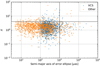 |
Fig. 1. Normalized separation between two decimation solutions as a function of the minimum semi-major axis of the error ellipse in the decimation solutions for VCS (blue asterisks) and other (brown triangles) sources. The horizontal line indicates the upper limit of X0 = 3.97 imposed on the individual normalized separation, while the vertical line shows the upper limit of 1 mas for the individual semi-major axis of the error ellipse, both for removing the outliers. |
3. Assessing the accuracy of solutions
3.1 Methods and results
Differences between source position estimates from two decimation solutions can be used to estimate the noise floor and scale factor. In the case of white noise measurements, the formal error of the radio source position is expected to decrease as  where N is the number of observations. If we have two solutions that are supposed to measure the same quantity, that is, the position of the same sources in this case, and that are also supposed to be of the same level of accuracy (e.g., because they have almost the same number of observations from equivalent VLBI networks), the position difference between the two solutions should tend toward zero when the number of observations increases. Here the wording “tend to zero” should be interpreted as “explained by the formal errors”. Statistically speaking, it means that the weighted root-mean-square (wrms) difference tends to zero as the number of observations increases or the wrms scatter is on the same order of the formal error. However, it is usually not the case because in the VLBI data reduction we assumed the distribution of measurement noise to be Gaussian-like and the modeling of the non-Gaussian errors, such as the station-dependent noise and modeling errors of troposphere parameters (e.g., see Gipson 2006; Romero-Wolf & Jacobs 2012), is not optimal. As pointed out in Ma et al. (2009), one of the motivations for inflating the formal errors and establishing a noise floor is to account for these non-Gaussian error sources.
Practically, we used two methods to determine the noise floor of the VLBI solution. One is to consider the noise floor as the minimum wrms scatter of the position differences as the number of the observations increases. Meanwhile, the scale factor s will be estimated as the standard deviation of the source position difference scaled by the combined formal error (root-sum-square of formal errors in two decimation solutions). This method is referred to as DSM. The main idea of the other method, is that if the combined formal error is under-estimated, the wrms scatter of the position differences will be larger than the error. A noise floor appears as a limit of the wrms scatter when the combined formal error decreases. We denoted the second method as SBL. Since we are interested in the noise floor of the two decimation solutions rather than their positional offset, and we assume that two solutions have the same level of noise, the wrms scatter and the combined formal error should both be scaled by  . For the sake of simplicity, the wrms and the combined formal error will implicitly refer to the ones scaled by
  in the remainder of this paper.
When we adopted the DSM method, the right ascension and declination component yielded a scale factor of 1.4 and 1.3, respectively. In order to determine the noise floor, we sorted the sources by the total number of sessions a source was observed in two decimation solutions and analyzed the wrms differences of source positions for subsets of every 50 sources in this ordered sequence. Figure 2 shows a decreasing tendency of the wrms scatter and median combined formal error as a function of the median number of sessions in the subset. The wrms scatter is generally larger than the formal error in right ascension, while for declination it occurs for the number of sessions larger than 100. One could see a minimum wrms scatter of about 8 μas in RA and 10 μas in Dec for sources that have been observed in about 1000 sessions. Compared with the ICRF2 catalog that shows a minimum wrms scatter of 15 μas for RA and 25 μas for Dec (Ma et al. 2009), our solutions show an improvement of a factor of nearly 2 for right ascension and 2.5 for declination. If the noise floor is measured by the minimum wrms, it could be ∼10 μas. This value, however, could be achieved for sources associated with a long observational history (e.g., being observed in more than 1000 sessions), which makes up only 8.4% of the clean sample. Compared to the reported noise floor for the ICRF3 which is 30 μas (Charlot 2018), this estimation looks like too optimistic. Another estimate is the wrms difference of the whole clean sample (709 sources), which is 20 μas for RA and 23 μas for Dec, respectively. As mentioned in the previous section, we removed the sources that have a low observational history (observed fewer than ten times). If we include these sources in the sample (2380 sources), the wrms difference for RA/Dec is 33/40 μas. The results are consistent with 30 μas, even though the wrms difference for all sources is larger. It is probably due to that different sessions or source sample were used in the ICRF3. Since the noise floor of the catalog should represent the noise of most sources, a conservative estimation of the noise floor could be 20 μas for RA and 23 μas for declination. We used the scale factor and noise floor obtained to inflate the formal errors according to Eq. (1) and plotted them in Fig. 2. We find that the inflated errors can account for the wrms scatters for most cases. We also note that for sources with number of observed sessions larger than 1000, the applied noise floor seems too large. It is, however, as expected since the applied wrms is too conservative for well-observed sources.
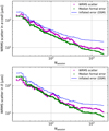 |
Fig. 2. Wrms scatter and median formal error of positional differences for subsets of every 50 sources binned by a sliding window as a function of the median number of sessions a source was observed in two decimation solutions. Also shown is the inflated median formal error inflated by the scale factor and noise floor of DSM. |
As for the SBL method, we sorted sources by their formal errors, binned them into subsets of every 50 sources, and calculated the wrms scatter and median combined formal error of position differences. Figure 3 presents the wrms scatter and median combined formal error for radio sources in each subset. We found a generally larger wrms scatter than the median combined formal error. Next we substituted the wrms scatter and median combined formal error for ξ and σ in Eq. (1) and performed the least square fitting. This yielded a scale factor of 1.2–1.3 and a noise floor of ∼10 μas in right ascension and declination. The estimated noise floor agrees with the minimum wrms in Fig. 2, implying that this method gives estimates of noise for a small subset of well-observed sources. We also note the large error of the noise floor estimate, which could lead to a noise floor of ∼20 μas in the worst case.
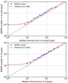 |
Fig. 3. Wrms scatter of source position differences as a function of the median formal error. Also shown for comparison is the inflated error using the scale factor and noise floor of SBL. |
To check our determination of the scale factor and noise floor, we then calculated the residual scale factor, that is, the standard deviation of the position differences scaled by the inflated errors. The closer to unity the residual scale factor is, the more realistic the scale factor and the noise floor is. Following such a philosophy, all the results are satisfactory both in right ascension and declination, showing a divergence of 0.1 from unity. Interestingly, the DSM method yielded a residual scale factor smaller than the unity while for the SBL it is slightly larger. From this point of view, the estimation from DSM might be over-estimated while the SBL method possibly under-estimates the scale factor and/or the noise.
All the results are summarized in Table 2. In short, the scale factor is estimated to be of about 1.3–1.4 for right ascension and 1.2–1.3 for declination; for noise floor, it is estimated to be lying between 20 μas and 25 μas in the two coordinates, showing an improvement of about 35% with respect to the ICRF2 catalog.
Scale factor and noise floor of formal errors.
3.2 Dependence on the number of observed sessions
In this section, we address the dependence of the scale factor on the number of sessions a source was observed and also check our results in Sect. 3.1. We grouped the sources similarly to the noise estimation of the DSM method (Sect. 3.1) and calculated the scale factor as the standard deviation of the normalized position differences. Figure 4 shows a mainly stable scale factor between 1.3 and 1.5 for right ascension and a general increasing scale factor in declination. We also rescaled the formal error using the results of DSM and SBL and calculated the residual scale factor. For both coordinates, the residual scale factor was reduced down to around 1.0 when the number of sessions is less than 100. More encouragingly, the increasing tendency of the scale factor in declination clearly vanished. In the case of Nsession ≥ 100, an obvious discrepancy between the results of DSM and SBL could be found. For the result of SBL, the residual scale factor was still consistent with the unity within 0.2, while the DSM method yielded a general decreasing trend from 1.0 to 0.5. Again, it suggests that for the sources with a rich observational history the noise floor is more close to 10 μas. This also indicates a promising future of the VLBI catalog which could reach the accuracy of 10 μas since new VLBI observations will be carried on continuously.
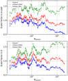 |
Fig. 4. Scale factors in right ascension and declination for subsets of 50 sources binned by a sliding window as a function of the median number of observed sessions. Also shown are the residual scale factors for DSM and SBL. |
3.3 Dependence on the declination
Since most VLBI sites are located in the northern hemisphere, the average formal error of radio source positions is generally better as the declination increases. As a result, we turned our interest to investigating the dependence of the scale factor and noise floor on the source declination. The scale factor (standard deviation of the normalized position differences) and wrms scatter were calculated for each 15° declination band.
As demonstrated in Fig. 5, the wrms scatter decreases with declination from nearly 55 μas to around 15 μas both in right ascension and declination, except for sources between −90° and −60°. The median wrms for declination bands in the south of the equator is 30/33 μas for RA/Dec while it is 16/19 μas in the north. It suggests that the noise level of position for sources in the southern hemisphere is about two times larger than that in the north. The right ascension shows a smaller wrms scatter compared to the declination, which is a chronic feature of VLBI. We note that for 555 sources (78% of the sample) locating in the north of 30° the wrms is the same as or better than 30 μas. This result agrees well with the reported noise floor of the ICRF3 (Charlot 2018). If one considers the peak of the distribution of numbers of source which is within 0–30° north, one could see a wrms lying between 20–25 μas for both coordinates, which is in good agreement with the estimation given by the DSM method.
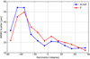 |
Fig. 5. Wrms scatter in right ascension and declination for each 15° declination band derived from source position differences between two decimation solutions. |
Figure 6 displays the scale factors for the 15 declination bands. For most declination bands, the scale factor in right ascension is quite uniform and stable around 1.4; for declination, the scale factor generally increases with the declination. Fey et al. (2015) showed a similar increasing scale factor as the declination both for right ascension and declination. The authors attributed this feature to the more observations for higher declination sources. To go further, we checked the residual scale factors using results of DSM and SBL (Table. 2). Contrary to the discrepancy shown in Fig. 4, these two methods show a general consistency within 0.1, even though SBL gives a larger residual scale factor. The residual scale factors in RA and Dec are well constrained within 0.8–1.0 for DSM and 1.0–1.2 for SBL for most declination bands. We note that for sources between 45–90° south the rescaling formal errors in declination are generally larger than the positional differences, indicating that the original declination formal errors for these sources may possibly be realistic.
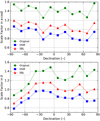 |
Fig. 6. Scale factor in right ascension and declination for each 15° declination band derived from source position differences between two decimation solutions. |
4. Comparison with ICRF2 and Gaia DR2 formal errors
In this section, we aim to compare the inflated formal error in the solution OPA by the scale factors and noise floors determined in Sect. 3.1, with the formal errors of the ICRF2 and Gaia DR2 catalogs. The OPA solution contains the positions of 4400 sources, with a median formal error of better than 100 μas in right ascension and ∼150 μas in declination (see Table 1). We inflated the formal errors of source position in OPA catalog with the results of DSM and SBL. For comparison, we used the ICRF2 catalog (Fey et al. 2015) and the gaiadr2.aux\_iers\_gdr2\_cross\_id catalog4, the latter containing the positions for the optical counterparts of 2820 VLBI sources at a reference epoch of J2015.5 (Gaia Collaboration 2018b) and labeled as Gaia DR2 for the sake of simplicity.
There are 2288 common sources among these three catalogs. Figure 7 reports the median formal errors in right ascension, declination, and the direction of the error ellipse major axis (EEMA) for these common sources. The inflated results from DSM and SBL yield a similar median formal error, which is ∼120–135 μas in right ascension and ∼190–220 μas in declination. One can notice that, after inflating the formal error, median errors in declination and EEMA of OPA are of the similar level as the Gaia DR2 but OPA provides a formal error that is better by a factor of about two in right ascension. Besides, OPA shows an improvement of a factor of ∼2.5 in right ascension, and of ∼3 in declination and EEMA with respect to the ICRF2 in terms of the median formal error. If we assume that the formal errors in ICRF2 and Gaia DR2, and inflated errors in OPA solution are realistic, we could conclude that current VLBI solutions still provide source positions with the best accuracy.
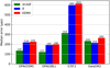 |
Fig. 7. Median error of the 2288 common sources among OPA solution, ICRF2 catalog, and Gaia DR2 catalog. EEMA represents the semi-major axis of error ellipse, which can be used to describe the positional formal error for a source. |
5. Concluding remarks
We proposed to estimate a realistic error of source positions in VLBI solution based on all the up-to-date VLBI observations. The scale factor is estimated to be of ∼1.3 in both coordinates. We found the noise floor to be of 20–25 μas for sources having been observed in more than ten sessions. If we take all the sources into consideration, the noise level could be worse. Nevertheless, this result shows an improved accuracy with respect to the ICRF2 and agrees well with the reported noise floor of the ICRF3 (Charlot 2018). For a small subset of well-observed sources (number of observed sessions larger than 1000), the noise floor of 10 μas could be reached, which shows a strong potential of the VLBI radio source catalog. Besides, the wrms noise is found to decrease from the southern to northern hemisphere, which is consistent with the result of ICRF2 (Fey et al. 2015). Typically, the positional accuracy in the northern hemisphere is about two times better than in the south. Taking the scale factor and noise floor into consideration, our solution shows a similar accuracy level to that of Gaia DR2 in declination but better by a factor of two in the right ascension. Our comparison also shows that nowadays the VLBI catalogs have been improved with respect to the ICRF2 catalog by a factor of three.
Acknowledgments
We thank an anonymous referee for their careful review and useful suggestions, which help improve the manuscript. N.L. was supported by the China Scholarship Council (CSC) for the joint doctoral training program at the SYRTE (Systèmes de Référence Temps-Espace) Department of the Paris Observatory (File No. 201706190125). N.L. is also funded by the National Natural Science Foundation of China (NSFC) under grant No. 111473013. This work has made use of data from the European Space Agency (ESA) mission Gaia (https://www.cosmos.esa.int/gaia), processed by the Gaia Data Processing and Analysis Consortium (DPAC, https://www.cosmos.esa.int/web/gaia/dpac/consortium). Funding for the DPAC was provided by national institutions, in particular the institutions participating in the Gaia Multilateral Agreement. This research has made use of NASA’s Astrophysics Data System. This research also made use of Matplotlib, an open-source 2D graphics package for Python (Hunter 2007).
Data publicly available at http://iers.obspm.fr/eop-pc
References
- Altamimi, Z., Rebischung, P., Métivier, L., & Collilieux, X. 2016, J. Geophys. Res. (Solid Earth), 121, 6109 [NASA ADS] [CrossRef] [Google Scholar]
- Boehm, J., Werl, B., & Schuh, H. 2006, J. Geophys. Res. (Solid Earth), 111, B02406 [NASA ADS] [CrossRef] [Google Scholar]
- Capitaine, N., Wallace, P. T., & Chapront, J. 2003, A&A, 412, 567 [NASA ADS] [CrossRef] [EDP Sciences] [Google Scholar]
- Charlot, P. 2018, in The Third Realization of the International Celestial Reference Frame, 30th IAU General Assembly [Google Scholar]
- Fey, A. L., Gordon, D., Jacobs, C. S., et al. 2015, AJ, 150, 58 [NASA ADS] [CrossRef] [Google Scholar]
- Frouard, J., Johnson, M. C., Fey, A., Makarov, V. V., & Dorland, B. N. 2018, AJ, 155, 229 [NASA ADS] [CrossRef] [Google Scholar]
- Gaia Collaboration (Prusti, T., et al.) 2016, A&A, 595, A1 [NASA ADS] [CrossRef] [EDP Sciences] [Google Scholar]
- Gaia Collaboration (Brown, A. G. A., et al.) 2018a, A&A, 616, A1 [NASA ADS] [CrossRef] [EDP Sciences] [Google Scholar]
- Gaia Collaboration (Mignard, F., et al.) 2018b, A&A, 616, A14 [NASA ADS] [CrossRef] [EDP Sciences] [Google Scholar]
- Gipson, J. M. 2006, in IVS 2006 General Meeting Proceedings, Concepción, Chile, March 2012, eds. D. Behrend, & K. Baver, 231 [Google Scholar]
- Gordon, D. 2017, J. Geod., 91, 735 [NASA ADS] [CrossRef] [Google Scholar]
- Gordon, D., Jacobs, C., Beasley, A., et al. 2016, AJ, 151, 154 [NASA ADS] [CrossRef] [Google Scholar]
- Herring, T. A., Mathews, P. M., & Buffett, B. A. 2002, J. Geophys. Res. (Solid Earth), 107, 2069 [NASA ADS] [CrossRef] [Google Scholar]
- Hunter, J. D. 2007, Comput. Sci. Eng., 9, 90 [NASA ADS] [CrossRef] [Google Scholar]
- Lambert, S. 2014, A&A, 570, A108 [NASA ADS] [CrossRef] [EDP Sciences] [Google Scholar]
- Lyard, F., Lefevre, F., Letellier, T., & Francis, O. 2006, Ocean Dyn., 56, 394 [NASA ADS] [CrossRef] [Google Scholar]
- Ma, C., Clark, T. A., Ryan, J. W., et al. 1986, AJ, 92, 1020 [NASA ADS] [CrossRef] [Google Scholar]
- Ma, C., Arias, E. F., Eubanks, T. M., et al. 1998, AJ, 116, 516 [NASA ADS] [CrossRef] [Google Scholar]
- Ma, C., Arias, E. F., Bianco, G., et al. 2009, IERS Technical Note, 35 [Google Scholar]
- Mathews, P. M., Herring, T. A., & Buffett, B. A. 2002, J. Geophys. Res. (Solid Earth), 107, 2068 [NASA ADS] [CrossRef] [Google Scholar]
- Mignard, F., Klioner, S., Lindegren, L., et al. 2016, A&A, 595, A5 [NASA ADS] [CrossRef] [EDP Sciences] [Google Scholar]
- Nothnagel, A. 2009, J. Geod., 83, 787 [NASA ADS] [CrossRef] [Google Scholar]
- Nothnagel, A., Artz, T., Behrend, D., & Malkin, Z. 2017, J. Geod., 91, 711 [NASA ADS] [CrossRef] [Google Scholar]
- Petrov, L., & Boy, J.-P. 2004, J. Geophys. Res. (Solid Earth), 109, B03405 [NASA ADS] [CrossRef] [Google Scholar]
- Romero-Wolf, A., & Jacobs, C. S. 2012, in IVS 2012 General Meeting Proceedings. Madrid, Spain, March 2012, eds. D. Behrend, & K. Baver, 231 [Google Scholar]
- Ryan, J., Clark, T., Ma, C., et al. 1993, Geodyn. Ser, 23, 37 [Google Scholar]
All Tables
All Figures
|
Fig. 1. Normalized separation between two decimation solutions as a function of the minimum semi-major axis of the error ellipse in the decimation solutions for VCS (blue asterisks) and other (brown triangles) sources. The horizontal line indicates the upper limit of X0 = 3.97 imposed on the individual normalized separation, while the vertical line shows the upper limit of 1 mas for the individual semi-major axis of the error ellipse, both for removing the outliers. |
| In the text | |
|
Fig. 2. Wrms scatter and median formal error of positional differences for subsets of every 50 sources binned by a sliding window as a function of the median number of sessions a source was observed in two decimation solutions. Also shown is the inflated median formal error inflated by the scale factor and noise floor of DSM. |
| In the text | |
|
Fig. 3. Wrms scatter of source position differences as a function of the median formal error. Also shown for comparison is the inflated error using the scale factor and noise floor of SBL. |
| In the text | |
|
Fig. 4. Scale factors in right ascension and declination for subsets of 50 sources binned by a sliding window as a function of the median number of observed sessions. Also shown are the residual scale factors for DSM and SBL. |
| In the text | |
|
Fig. 5. Wrms scatter in right ascension and declination for each 15° declination band derived from source position differences between two decimation solutions. |
| In the text | |
|
Fig. 6. Scale factor in right ascension and declination for each 15° declination band derived from source position differences between two decimation solutions. |
| In the text | |
|
Fig. 7. Median error of the 2288 common sources among OPA solution, ICRF2 catalog, and Gaia DR2 catalog. EEMA represents the semi-major axis of error ellipse, which can be used to describe the positional formal error for a source. |
| In the text | |
Current usage metrics show cumulative count of Article Views (full-text article views including HTML views, PDF and ePub downloads, according to the available data) and Abstracts Views on Vision4Press platform.
Data correspond to usage on the plateform after 2015. The current usage metrics is available 48-96 hours after online publication and is updated daily on week days.
Initial download of the metrics may take a while.