| Issue |
A&A
Volume 620, December 2018
|
|
|---|---|---|
| Article Number | A129 | |
| Number of page(s) | 9 | |
| Section | Astrophysical processes | |
| DOI | https://doi.org/10.1051/0004-6361/201834000 | |
| Published online | 07 December 2018 | |
Modelling the disc atmosphere of the low mass X-ray binary EXO 0748-676
1
SRON Netherlands Institute for Space Research, Sorbonnelaan 2, 3584 CA
Utrecht, The Netherlands
e-mail: This email address is being protected from spambots. You need JavaScript enabled to view it.
2
ESO, Karl-Schwarzschild-Strasse 2, 85748
Garching bei Munchen, Germany
Received:
1
August
2018
Accepted:
13
September
2018
Abstract
Low mass X-ray binaries exhibit ionized emission from an extended disc atmosphere that surrounds the accretion disc. However, the atmosphere’s nature and geometry is still unclear. In this work we present a spectral analysis of the extended atmosphere of EXO 0748-676 using high-resolution spectra from archival XMM-Newton observations. We model the spectrum that is obtained during the eclipses. This enables us to model the emission lines that come only from the extended atmosphere of the source, and study its physical structure and properties. The RGS spectrum reveals a series of emission lines consistent with transitions of OVIII, OVII, NeIX and NVII. We perform both Gaussian line fitting and photoionization modelling. Our results suggest that there are two photoionization gas components that are out of pressure equilibrium with respect to each other. One has an ionization parameter of log ξ ∼ 2.5 and a large opening angle, and one has log ξ ∼ 1.3. The second component possibly covers a smaller fraction of the source. From the density diagnostics of the OVII triplet using photoionization modelling, we detect a rather high density plasma of > 1013 cm−3 for the lower ionization component. This latter component also displays an inflow velocity. We propose a scenario where the high ionization component constitutes an extended upper atmosphere of the accretion disc. The lower ionization component may instead be a clumpy gas created from the impact of the accretion stream with the disc.
Key words: techniques: spectroscopic / binaries: eclipsing / X-rays: binaries / X-rays: individuals: EXO 0748-676
© ESO 2018
1. Introduction
Low mass X-ray binaries display remarkable physical phenomena such as accretion, winds, plasma heating, time variability and magnetic fields. An accretion disc of an X-ray irradiating plasma encircles the central compact source of the system. Some of these systems present a thickened accretion disc with material that extends above the disc midplane, the so-called accretion disc corona (ADC or hereafter extended disc atmosphere). The nature and exact geometry of this extended atmosphere is not yet fully understood.
To this end, different theoretical models predict the existence of a disc atmosphere. White & Holt (1982) studied the accretion disc corona and predicted that it is probably generated by evaporation of hot material from the surface of the accretion disc. Later, Miller & Stone (2000) using magnetohydrodynamic (MHD) models showed that an initially weak magnetic field in the core of the disc can be amplified by MHD turbulence driven by magnetorotational instabilities. This field rises out of the disc through buoyancy, creating a magnetised heated corona above the disc at 2–5 scale heights and a corona temperature of ∼108 K. Jimenez-Garate et al. (2002) modelled both the accretion disc atmosphere and the corona, photoionized by a central X-ray source. They found that the vertical scale height of the accretion disc atmosphere is enlarged by illumination heating. In this case the atmosphere is orders of magnitude less dense than the disc itself.
Observational studies have also revealed the existence of an extended atmosphere for a number of sources. Using high-resolution X-ray spectroscopy it is possible to identify emission and absorption lines within the disc plasma and around it. Cottam et al. (2001a) studied the XMM-Newton RGS (Reflection Grating Spectrometer) spectrum of EXO 0748-676 and found emission and absorption features (OVIII, OVII, NeIX, NVII) from an extended, oblate structure above the accretion disc. Further, Jimenez-Garate et al. (2003) examined the Chandra spectrum of the same source and found photoionized plasma located above the disc midplane. Also insights have been gained from the spectrum of other accretion disc corona (ADC) sources. Sources 4U 1822-37 (Cottam et al. 2001b), 2S 0921-63 (Kallman et al. 2003) and Hercules X-1 (Jimenez- Garate et al. 2005) have been studied using Chandra observations. For all these sources spectral signatures of an extended disc atmosphere were found. Noticeably, all the systems above are at high inclination angles.
Furthermore, the light curve of low mass X-ray binaries can reveal events such as dips, bursts, and eclipses. Dips and eclipses are shown in the light curve as an abrupt drop in the count-rate (see Fig. 1). Eclipses are caused when the companion star is passing in front of the compact object and hides the emission of the disc, while the dips can be created due to over-densities from the impact of the accretion stream and the disc (Jimenez-Garate et al. 2002). It was found that only a group of low mass X-ray binaries with high-inclination (i ∼ 70 ° −90°) present dips and eclipses (Frank et al. 1987; Diaz Trigo et al. 2006). Among the 13 listed low mass x-ray binaries (LMXBs) with high-inclination, only a few of them show eclipses, for example EXO 0748-676 (Parmar et al. 1986) and MXB 1659-298 (Sidoli et al. 2001).
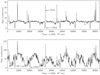 |
Fig. 1. Upper panel: light curve of a single observation showing the eclipses and bursts in the hard band (5–10 keV). Lower panel: light curve for the same observation including dips, eclipses and bursts in the soft band (0.3–5 keV). Obs. ID: 0160760201. |
EXO 0748-676 is an LMXB discovered in 1985 by the European X-ray Observatory Satellite (EXOSAT). This source was used as a calibration source of XMM-Newton satellite and it has been observed and studied extensively by different satellites (Parmar et al. 1991; Hertz et al. 1995; Hertz et al. 1997; Thomas et al. 1997; Church et al. 1998; Jimenez-Garate et al. 2003; Sidoli et al. 2005; Wolff et al. 2005; van Peet et al. 2009).
Parmar et al. (1986) discovered periodic intensity dips. Eclipses of this source display a period of 3.82 h lasting 8.3 min. The mass of the companion is reported to be 0.08 M⊙ < Mc < 0.45 M⊙ and the inclination of the system is 75 ° < i < 83° (Parmar et al. 1986). The radial velocity is 20 km s−1 (Duflot et al. 1995). The distance of the source was derived to be [5.8 ± 0.9 kpc] or [7.7 ± 0.9 kpc] depending on whether the X-ray bursts of the source are hydrogen-dominated or helium-dominated respectively (Wolff et al. 2005). Here, we use the average value of 6.8 kpc.
In this work, we have analysed the XMM-Newton data of EXO 0748-676 during the eclipses. This is the first time that the spectrum from only the extended atmosphere of the disc is being studied for this source. In that way we can understand the emission that comes from the upper disc atmosphere and also its geometry. In previous studies, the density of the plasma has been derived by comparing line ratios of the OVII triplet with theoretical calculations (see Porquet & Dubau 2000). In our study we constrain the density directly using photoionization modelling in SPEX as described in Sect. 3. This paper is organised as follows. In Sect. 2 we present the data and the XMM-Newton data reduction and we explain the methodology used to obtain the RGS spectrum of the eclipses. In Sect. 3 we present the Gaussian line fitting and the photoionization modelling of the eclipsed spectrum. Finally in Sect. 4 we discuss the results, proposing a geometry for the X-ray emitting gas.
2. XMM-Newton data reduction
We use data from european photon imaging camera (EPIC) with the pn (Struder et al. 2001) and MOS (Turner et al. 2001) cameras and the RGS spectrometer (den Herder et al. 2001), taken from the XMM-Newton public archive1. We reduce the data using the Science Analysis Software, SAS (ver. 16). First, we filter the EPIC event lists for flaring particle background. We exclude the observations with flaring particle background exceeding 0.4 counts/s for pn and 0.35 for MOS.
To extract the light-curve we use a circular aperture (R ∼ 30″) around the source. For the background we use a circular aperture of the same size away from the source but within the same chip. We selected energies between 5 and 10 keV. This allowed us to clearly identify the eclipse events. At softer energies the contribution of the dipping events to the light curve becomes relevant, possibly confusing the selection. The light curve of the source is corrected for various effects on the detection efficiency such as vignetting, quantum efficiency and bad pixels, using the SAS task epiclccorr. An example of a corrected light curve is shown in Fig. 1. In the upper panel we see the light curve of the eclipses and bursts with a 5 < E (keV) < 10 energy selection. In the lower panel we present also the dipping events, obtained in the energy range 0.3–5 keV, and we will discusse them in Sect. 4.1.2. We call the periods outside these events “persistent emission”.
We use in total 11 observations obtained in three different years, presented in Table 1. Depending on the availability of the data and the quality of the light curve, we use the EPIC-pn or EPIC-MOS data to obtain the good time intervals (GTI) for the emission during the eclipses. We use these GTIs to extract the RGS spectrum at the time of the eclipses. We choose the best observations according to the quality of the light curves: the count rate (counts/sec) of the persistent emission in the light curve should be at least two times higher than the eclipses. After that, we process the RGS data using the SAS task rgsproc. We also use a geometrical binning of a factor of three, which provides a bin size of about 1/3 of the RGS resolution.
Log of XMM-Newton observations used in this paper.
The eclipsed RGS spectra from different years do not present significant variability within the errors. Therefore, we combine the observations using the SAS task rgscombine to obtain a better signal-to-noise ratio. We also use a single EPIC-pn observation to create the spectrum of the EPIC-pn persistent emission and to obtain the continuum parameters. This is useful in order to obtain the correct spectral energy distribution (SED) of the illuminating source which will be discussed in Sect. 3.
3. Modelling the eclipsed spectrum
We fit the combined RGS spectrum using the X-ray fitting package SPEX (Kaastra et al. 1996, ver. 3.04). We perform a time averaged analysis of the spectrum. In Fig. 2 we present the eclipsed spectrum of the source obtained as described in Sect. 2. The observed continuum is extremely low due to the fact that the persistent continuum from the disc and the neutron star is blocked during the eclipse. From the spectrum we can clearly see interesting features such as the emission lines in OVIII (18.97 Å) and the OVII triplet (21.6–22.1 Å). For a detailed study of the spectrum we perform a Gaussian line detection and then we model the eclipsed spectrum of the source using a global modelling.
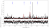 |
Fig. 2. Eclipsed spectrum of EXO 0748-676 with Gaussian modelling and residuals. The line at 23 Å corresponds to a bad pixel. |
3.1. Line detection
First, we apply an RGS line detection in the 7–37 Å wavelength range following the method described in Pinto et al. (2016). This will help us to identify fainter lines in our low flux spectrum. We scan the spectrum using Gaussians (component gaus in SPEX) in order to identify the lines with the highest significance. We apply a scanning step of 0.025 Å and fix the width of the Gaussian line at 0.005 Å. In Fig. 3 we present the result from the line scanning, where the ΔCstat is multiplied by the sign of the Gaussian normalisation. The red line indicates the level of 3σ detection. From the scan we can clearly see the lines at 18.97 Å and at (21.6–22.1) Å, which correspond to OVIII and OVII respectively, and present the highest significance. Also, with lower significance level (but > 3σ), we observe the NeIX line at 13.4 Å and NVII at 24.7 Å.
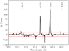 |
Fig. 3. Gaussian line scanning to detect the strongest lines. The red dashed lines correspond to the 3σ detection level. The very narrow absorption-like features correspond to bad pixels. |
3.2. Gaussian line fitting
We now apply a Gaussian line fitting to parametrise our emission lines in a model independent way and determine the kinematics of our spectrum. We begin with the simple approach of a power-law continuum and Gaussian line profiles. In this way we can obtain the strength of the lines and their velocities. We use a power-law continuum model for the continuum and the hot model in SPEX in order to take into account the Galactic absorption. For the column density we use the Galactic value 3.5 × 1021 cm−2 (Kalberla et al. 2005). In Table 2 we present the results of the fitting and in Fig. 2 we present the best fit.
Gaussian modelling parameters of the emission lines detected in the RGS spectrum.
The width of the lines in some cases could not be resolved. For this reason we couple the widths of the forbidden and the recombination lines to the width of the intercombination line for each of our triplets, OVII and NeIX. Also we keep the theoretical values for the wavelength in most of our lines but we apply a redshift component in SPEX for these lines to take into account a possible line shift. We apply different redshift for the OVII and NeIX triplets. We observe our lines slightly redshifted. In Table 2 we present the velocity shift (vflow) and broadening (σ) for each line. The velocity shifts of the lines are comparable. Especially the low ionization (OVII) and high ionization (OVIII) lines present the same kinematics. Within the errors, a moderate inflow is detected.
From the flux of the lines in the OVII triplet, we calculate the G and R ratios. These ratios are plasma diagnostics and can be used to identify the photoionized plasma (Liedahl 1999; Mewe & Schrijver 1978). The G ratio is sensitive to the electronic temperature while the R ratio is sensitive to the electronic density (Gabriel & Jordan 1969) and they are given by
 (1)
(1)
 (2)
(2)
where f, i, and r represent the flux of the forbidden, intercombination, and resonance line, respectively. The G ratio is ∼ 4, which indicates photoionized gas (Porquet & Dubau 2000). The R ratio is ∼0.02 indicating a high electron density > 1012 cm−3 (Fig. 8 of Porquet & Dubau 2000).
3.3. Photoionization modelling
Next, we perform a detailed spectral analysis using a photoionization model. We apply the models for the RGS wavelength range, 7–35 Å. In order to fit the emission features we use the pion model in SPEX2 (see Mehdipour et al. 2016). Pion is a photoionization plasma model where the photoionization equilibrium is calculated self-consistently.
3.3.1. Spectral energy distribution
To obtain the correct spectral energy distribution (SED) of the central source we use the following approach. During the eclipses the ionizing continuum is shielded and is not visible in the eclipsed spectrum. Thus, we fit the EPIC-pn spectrum of a single observation, during the persistent phase, to obtain the parameters of the ionizing continuum. The best fit of the persistent emission is shown in Fig. 4. We apply a power law and a black body. For a better fit of the absorption and emission features we also add a hot component for the Galactic absorption. We also use a xabs component. Xabs is a photoionized absorption model and calculates the transmission of a slab of material. It is needed to fit the ionized gas seen in the persistent spectrum of this source, as described in van Peet et al. (2009). Xabs is a fast fitting model that contains only absorption lines while pion contains also lines in emission. Thus, it is useful to fit the pn spectrum with xabs where we cannot see the emission lines because of the moderate resolution of the instrument. The parameters of the fit are listed in Table 3.
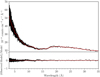 |
Fig. 4. Best fit of the EPIC-pn persistent spectrum and residuals (Obs ID: 0160761301). |
Continuum parameters of the spectrum during the persistent emission and the power-law parameters resulting from the eclipsed spectrum.
The emission lines that are present in the “eclipsed” RGS spectrum are photoionized by the continuum that is seen during the “persistent” phase. Therefore, for our pion modelling we use the continuum model that we derived from the EPIC-pn spectrum taken during the persistent phase. This continuum is of course different from the low-level observed continuum during the eclipsed phase. Thus, in our SPEX modelling of the eclipsed RGS spectrum, we prevent the persistent continuum from being observed, which is done by incorporating an etau model. We note that additional etau2 components are used to create the low-energy and high-energy exponential cut-off of the power-law component of the persistent continuum. A high-energy cut-off was applied at 100 keV and a low energy at 13.6 eV.
3.3.2. Fitting the eclipsed emission
We fit the following parameters of the pion model in SPEX. First, we fit the ionization parameter ξ = L/nH ⋅ r2 where L is the source luminosity and r the distance from the ionizing source. The hydrogen column density NH in cm−2 and the plasma density nH in cm−3 are also fitted. Further we fit the parameter Ω/4π, which gives the opening angle of our plasma material divided by 4π, the velocity shift vflow, and the broadening σ in km s−1.
The OVIII line prevents the OVII from being properly fitted when only one photoionization component is applied. For this reason, we need two pion components with different ionization parameters to fit the highly ionized and the weakly ionized lines (hereafter, component A and B respectively). A comparison between the modelling with one and two pion components is presented in Fig. 5, lower panel.
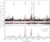 |
Fig. 5. Upper panel: best fit spectrum of EXO 0746-676 using 2 pion components. The feature at 23 Å corresponds to a bad pixel. Middle panel: residuals. Lower panel: pion emission components. The combination of 2 components can fit best both OVII and OVIII. |
The best fit is shown in Fig. 5 and the best-fit parameters for the two photoionization components in Table 4. The OVII triplet (component B) is very sensitive to the density of the plasma. In our model, we applied a density grid starting from a low value of ∼1 cm−3 to see the effect of using lower and higher densities. In Fig. 6 we present the zoom-in of the OVII region using the models with different density. The best fit to the data gives a rather high density of 2 × 1013 cm−3 for component B (upper limit). Also in our case, the OVII intercombination line seems to be the strongest and the forbidden line seems to be suppressed, which is what we expect for a high density gas (Porquet & Dubau 2000). On the other hand, for component A we cannot constrain a value of density due to poor signal-to-noise around the NeIX region. The OVIII and NeIX lines are not affected by the density changes. For this reason the densities of components A and B are coupled. We observe a net gas velocity of ∼ + 800 km s−1 (from component B) which indicates an inflowing gas towards the disc. For component A the velocity cannot be constrained. We derive a different ionization parameter and opening angle (Ω) for the two components. In our spectrum, we also detect the OVII and OVIII radiative recombination continuum feature (RRC) at 16.75 Å and 14.20 Å respectively. These narrow features are an indication of photoionized gas (van Paradijs & Bleeker 1998; Jimenez-Garate et al. 2003). Furthermore, knowing the ionization parameter and the density, we calculate the emission measure (EM) for the two photoionization components (see Tables 4 and 5). Knowing the distance from the ionization source from the equation:
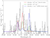 |
Fig. 6. OVII spectral range and model calculation with different densities. The best fit is given from the higher density value, displayed in red. |
Best-fit parameters of the pion photoionization model components fitted to the stacked XMM-Newton data.
 (3)
(3)
we then calculate the emission measure using the formula (see e.g. Mao et al. 2017)
 (4)
(4)
where nH, NH, and ne are the density, the column density and the electron density, respectively and Ω is the opening angle.
3.3.3. Testing for alternative models
Here, we test whether collisional-ionization equilibrium provides a better description of the data. Therefore, we fitted our eclipsed spectrum with the cie model in SPEX, which fits the spectrum of plasma in a collisionally equilibrium state. We use the same continuum (as described in Sect. 3.3.1) and fit two cie components. We also add a reds component in SPEX to take into account the possible redshift of the lines. We found a different plasma temperature for each cie component, 5 keV and 0.15 keV, respectively. In this model, we notice that the forbidden line is strong and the intercombination is suppressed, which does not represent our case. We conclude that a low-density collisionally ionized gas is not valid in this case. We test also a high-density collisionally-ionized gas, which also does not fit better in our spectrum (C-stat/Exp. C-stat = 1842/1067). Furthermore, in the cie model, one can test the case of non-equilibrium plasma. We let free the parameter rt (the ratio of ionization balance to electron temperature). The electron density for both components is ∼3 × 1013 cm−3. In this case, the intercombination line becomes stronger than the resonance and the forbidden is suppressed, but we still do not obtain a better fit than the photoionized case, as we see in Fig. 7 (C-stat/Exp. C-stat = 1738/1067). Lastly, we tested the possibility of a more complicated model which is the combination of a collisionally ionized component and a photoionization component, in order to reduce our residuals. It still does not improve our fit so we conclude that the best-fit model that represents our case is photoionization modelling.
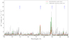 |
Fig. 7. Modelling the eclipsed spectrum of EXO 0748-676 with collisionally ionized gas and comparison to the best-fit photoionized gas. In both cases we have a high-density gas. |
3.4. Are the two photoionization components thermally stable?
A photoionized plasma can be unstable at some ionization states. We test whether our photoionization components are in pressure equilibrium. This can be tested by creating a stability curve (called also S-curve or cooling curve). The stability curve shows the change in the electron temperature as a function of the pressure form of the ionization parameter Ξ, introduced by Krolik et al. (1981), which is defined as the radiation pressure divided by the gas pressure.
We produce the S-curves as follows. We first create a grid of electron temperatures and ionization parameter ξ according to our photoionization modelling and the SED in SPEX. Further we calculate the pressure, Ξ. The parameter Ξ gives the ionization equilibrium and can be expressed as Ξ = F/nH ⋅ c ⋅ kT, where nH is the hydrogen density in cm−3, k is the Boltzmann constant, and T the gas temperature. Since F = L/4 ⋅ π ⋅ r2 and ξ = L/nH ⋅ r2, Ξ can be written as
 (5)
(5)
In Fig. 8 we present the stability curve. We also overplot with empty and filled circles the location of our photoionization components A and B, respectively. The two components are not in pressure equilibrium. Component B is cooler and it belongs to a thermally stable part of the curve. Component A is hotter and it may reside on a thermally unstable branch, although from the position of the component on the curve this is difficult to constrain.
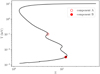 |
Fig. 8. Thermal stability curve of the photoionization modelling. The two components are not in pressure equilibrium. |
4. Discussion
In this work, we performed a spectroscopic study of the eclipsed spectrum of the low mass X-ray binary EXO 0748-676. We fit the spectrum using both Gaussian line modelling and photoionization modelling. By modelling the eclipsed spectrum we isolate only the material that comes from the area that surrounds the disc, from which we confirm the existence of an upper extended disc atmosphere.
4.1. Geometry of the system
4.1.1. The observed two-phase gas
In our analysis we performed photoionization modelling using two components in order to fit both the lower (OVII) and higher ionization (OVIII) lines (see Fig. 5). The Gaussian line fitting and G ratio indicate the existence of photoionized emission from the upper disc atmosphere. Also, with our global modelling, we found narrow radiative recombination continuum (RRC) features in the spectrum. The RRC emission features in the spectrum show that photoionization is the dominant ionizing mechanism in the plasma. Thus, we support our initial assumption for using photoionization modelling.
From the stability curve (see Sect. 3.4) we see that we have a two-phase gas out of pressure equilibrium. This may suggest that components A and B (see Table 4) are independent gas components. Looking at the fitting parameters in Table 4, the two components have different ionization (ξ) and opening angle (Ω). The higher ionization component (A) comes from a region with an opening angle of 2 ⋅ π while the lower ionization one (B) comes from a region two orders of magnitudes smaller. We also find a rather high density for component B (∼1013 cm−3) while for component A the density could not be determined due to poor signal-to-noise around the NeIX region. Component B seems to be also inflowing. For component A the velocity cannot be constrained.
4.1.2. The structure of the atmosphere
In Fig. 9 we present an illustration that shows the position of the two-phase gas and the shape of the upper atmosphere which most likely fit to our case. From our observational results we see a two-phase gas covering a different area along the line of sight. The emission measure for the lower ionization component (B) is smaller than that of the higher one (A) (see Table 5). From the definition of the emission measure (EM = ∫nenHdV), we can conclude that the gas of component B is coming from a small volume that is consistent with the small value of Ω, while component A is covering a broader area.
 |
Fig. 9. Illustration of EXO 0748-676 with the clumps in the extended atmosphere. Symbols A and B show the emission regions of our two photoionization components. A is the hotter component while B is the cooler one. The components in the figure are not to scale. |
Calculated parameters according to the best-fit parameters of the pion photoionization model components fitted to the stacked XMM-Newton data.
A likely scenario that explains the above results is the following. The high ξ and larger Ω material comes from the extended atmosphere that is located above the accretion disc. This atmosphere can be created by illumination that comes from the disc which is heated by the central X-ray source (see Jimenez-Garate et al. 2003).
The material that we see during the eclipse, and refer to as component B, can be related to the material impinging on the disc. Interestingly, the eclipses systematically come during the dipping event, almost at the end of it (see Fig. 1, lower panel). This applies to all our observations. Most dips are observed to be over-densities above the disc region (at the outer disc edge), which has been thickened as an effect of the impact with the accretion stream (White & Swank 1982; Frank et al. 1987). Diaz Trigo et al. 1987 found that in the low mass X-ray binary system XB 1254-690, the gas in the line of sight causing the dips is clumpy. Clumps have also been suggested to explain the phenomenology seen in Her X-1 (Schandl 1996) or to explain the high optical luminosity of supersoft X-ray sources (Suleimanov et al. 2003). In our case, the lower ξ gas with the small volume may come from a clumpy region above the disc. This emission could come from a clumpy gas that may have been created due to pressure instabilities during the impact of the accretion stream and the disc. The clumps seem to have a rather high density (∼1013 cm−3) and also they might have an inflowing velocity. This geometrical picture can explain also our findings for a two-phase gas.
The atmosphere (component A in Fig. 9) is most likely extended in the outer region of the disc. We can explain the existence of an extended corona in the frame of X-ray irradiation of the upper layers of an accretion disc (see e.g. Jimenez-Garate et al. 2002). In this context, in the inner region of the accretion disc, close to the neutron star, viscous heating is the dominant heating mechanism. The outer region of the accretion disc is dominated by external illumination and thus radiative heating exceeds viscous heating. The X-ray field of the neutron star photoionizes and heats the gas. Additional heating also is provided by the illumination from the accretion stream. The gas tends to move towards a situation of hydrostatic equilibrium, convection is suppressed and the disc increases the scale height. For this reason the geometry of the extended atmosphere is more extended in the outer part of the disc.
4.2. Comparison with previous results
We compare the spectroscopic results of EXO 0748-676 with results from other sources that present an extended accretion disc corona. Kallman et al. (2003) analysed Chandra observations from the high-inclination ADC source 2S 0921-63. From the density diagnostics in OVII line, they constrain a density for the ADC of 109 − 1011 cm−3 and the ionization parameter, log ξ = 2.
Cottam et al. (2001b) found from the Chandra spectrum of the ADC source 4U 1822-37 an opening angle of  which, according to the authors, constrains an extended area around the source. Also they derive an electron density of 1011 cm−3. Jimenez- Garate et al. (2005), for the ADC source Hercules X-1, obtained using the R-ratio a high density of 1013 cm−3, similar to the value obtained here. According to the authors, this density is consistent also with predicted atmospheric models. Also, in both sources, the presence of the RRC emission features is evident.
Cottam et al. (2001a) studied the XMM-Newton spectrum during the persistent emission intervals of EXO 0748-67 and found emission lines from OVII, OVIII, NeIX, and NeVII. They conclude that these features are coming from the extended atmosphere above the disc. They estimate the density using the line ratios and they found a lower limit for OVII and NeIX of 2 × 1012 cm−3 and 7 × 1012 cm−3. They also found the velocity broadening of the Lyα of OVIII ∼ 1400kms−1 and a systemic velocity of the emitting plasma < 300 km s−1.
Jimenez-Garate et al. (2003) analysed the persistent Chandra spectrum of EXO 0748-676 and confirmed the existence of an upper atmosphere around the disc. They found the upper atmosphere to extend 8 ° −15° with respect to the disc midplane. Furthermore, the density measured from the OVII lines is ∼1011 cm−3 and there is a mean broadening of the brightest lines of ∼700 km s−1. Their lines seem to be at rest, while our modelling shows a slight redshift. It has to be noted that in this case the authors studied the total emission of the disc in the persistent interval while in our case we get the emission only from the upper disc atmosphere and at a specific time interval of the accretion event.
5. Summary
In this study we have analysed the XMM-Newton RGS spectrum of the low mass X-ray binary EXO 0748-676 during the eclipses. This allowed us to study for the first time the gas coming only from the upper disc atmosphere. In our work, we modelled the emission lines using Gaussian line fitting to estimate the gas velocity and line shift in a model-independent way. Furthermore, we used photoionization modelling and constrained the density and the structure of the atmosphere. Our conclusions are the following:
-
We confirm the existence of an extended atmosphere above the accretion disc of EXO 0748-676. We detect OVII and OVIII lines with high significance but also NeIX and NVII lines. We measure positive velocity shifts for the strongest lines, which gives evidence for inflowing gas towards the central source.
-
From the line ratios of the OVII triplet and the photoionization modelling, we estimate the density of the gas and we obtain a rather high value of ∼1013 cm−3.
-
In our modelling we use two photoionization components. Our thermal stability analysis shows that the two components are out of equilibrium with each other. This means that we probably observe two distinct gas components. One displays smaller opening angle and comes most likely from clumps created from the impact of the accretion stream with the disc, inflowing towards the source. The other belongs to the atmosphere and from our modelling we find that it covers an area of at most 2π.
-
The results support the scenario that the extended disc atmosphere is created due to the heating of the outer part of the disc from the central compact source and the accretion stream and it is most likely photoionized.
Acknowledgments
The authors thank the anonymous referee for the useful comments. IP, DR, and EC are supported by the Netherlands Organisation for Scientific Research (NWO) through The Innovational Research Incentives Scheme Vidi grant 639.042.525. The Space Research Organization of the Netherlands is supported financially by the NWO. We would like to thank R. Waters for constructive suggestions on the manuscript and C. Done for useful discussions on the shape of the disc atmosphere. We also thank I. Urdampilleta for providing help with python and C. Pinto for advice on the line detection.
References
- Church, M. J., Bałucińska-Church, M., Dotani, T., & Asai, K. 1998, ApJ, 504, 516 [NASA ADS] [CrossRef] [Google Scholar]
- Cottam, J., Kahn, S. M., Brinkman, A. C., den Herder, J. W., & Erd, C. 2001a, A&A, 365, L277 [NASA ADS] [CrossRef] [EDP Sciences] [Google Scholar]
- Cottam, J., Sako, M., Kahn, S. M., & Paerels, F. 2001b, ApJ, 557, L101 [NASA ADS] [CrossRef] [Google Scholar]
- den Herder, J. W., Brinkman, A. C., Kahn, S. M., et al. 2001, A&A, 365, L7 [NASA ADS] [CrossRef] [EDP Sciences] [Google Scholar]
- Diaz Trigo, M., Parmar, A. N., Boirin, L., et al. 1987, A&A, 178, 137 [Google Scholar]
- Diaz Trigo, M., Parmar, A. N., Boirin, L., Mendez, M., & Kaastra, J. S. 2006, A&A, 445, 179 [NASA ADS] [CrossRef] [EDP Sciences] [Google Scholar]
- Duflot, M., Figon, P., & Meyssonnier, N. 1995, A&A, 114, 269 [Google Scholar]
- Frank, J., King, A. R., & Lasota, J. P. 1987, A&A, 178, 137 [NASA ADS] [Google Scholar]
- Gabriel, A. H., & Jordan, C. 1969, MNRAS, 145, 241 [NASA ADS] [CrossRef] [Google Scholar]
- Gottwald, M., Haberl, F., Parmar, A. N., & White, A. E. 1986, ApJ, 308, 213 [NASA ADS] [CrossRef] [Google Scholar]
- Hertz, P., Wood, K. S., Cominsky, L. 1995, ApJ, 438, 385 [NASA ADS] [CrossRef] [Google Scholar]
- Hertz, P., Wood, K. S., & Cominsky, L. 1997, ApJ, 486, 1000 [NASA ADS] [CrossRef] [Google Scholar]
- Jimenez-Garate, M. A., Raymond, J. C., & Liedahl, D. A. 2002, ApJ, 581, 1297 [NASA ADS] [CrossRef] [Google Scholar]
- Jimenez-Garate, M. A., Schulz, N. S., & Marshall, H. L. 2003, ApJ, 590, 432 [NASA ADS] [CrossRef] [Google Scholar]
- Jimenez-Garate, M. A., Raymond, L. C., Liedahl, D. A., & Hailey, C. J. 2005, 625, 931 [Google Scholar]
- Kaastra, J. 2017, A&A, 605, A51 [NASA ADS] [CrossRef] [EDP Sciences] [Google Scholar]
- Kaastra, J. S., Mewe, R., & Nieuwenhuijzen, H. 1996, UV and X-ray Spectroscopy of Astrophysical and Laboratory Plasmas, 411 [Google Scholar]
- Kalberla, P. M. W., Burton, W. B., Hartman D., Arnal, E. M., & Bajaja, E. 2005, A&A, 440, 775 [NASA ADS] [CrossRef] [EDP Sciences] [Google Scholar]
- Kallman, T. R., Anglelini, L., Borson, B., & Cottam, J., 2003, ApJ, 583, 861 [NASA ADS] [CrossRef] [Google Scholar]
- Krolik, J. H., McKee, C. F., & Tarter, C. B. 1981, ApJ, 249, 422 [NASA ADS] [CrossRef] [Google Scholar]
- Liedahl, D. A. 1999, in X-ray Spectroscopy and Astrophysics (Berlin: Springer), eds. J. A. van Paradijs, & J. A. M. Bleeker, Proc. EADN School, 189 [Google Scholar]
- Mao, J., Kaastra J. S., Mehdipour M., et al. 2017, A&A, 612, A18 [Google Scholar]
- Mehdipour, M., Kaastra, J., & Kallman, T. 2016, A&A, 596, A65 [NASA ADS] [CrossRef] [EDP Sciences] [Google Scholar]
- Mewe, R., & Schrijver, J. 1978, A&A, 65, 99 [NASA ADS] [Google Scholar]
- Miller, K. A., & Stone, J. M. 2000, ApJ, 534, 398 [NASA ADS] [CrossRef] [Google Scholar]
- Parmar, A. N., White, N. E., Giommi, P., & Gottwald, M. 1986, ApJ, 308, 199 [NASA ADS] [CrossRef] [Google Scholar]
- Parmar, A. N., Smale, A. N., Verbunt, F., & Corbet, R. H. D. 1991, ApJ, 366, 253 [NASA ADS] [CrossRef] [Google Scholar]
- Pinto, C., Middleton, M. J., & Fabian, A. C. 2016, Nature, 533, 64 [NASA ADS] [CrossRef] [Google Scholar]
- Porquet D., & Dubau J. 2000, A&AS, 143, 495 [NASA ADS] [CrossRef] [EDP Sciences] [Google Scholar]
- Schandl, S. 1996, A&A, 307, 95 [NASA ADS] [Google Scholar]
- Sidoli, L., Oosterbroek, T., Parmar, A. N., Lumb, D., & Erd, C. 2001, A&A, 379, 570 [Google Scholar]
- Sidoli, L., Parmar, A. N., & Oosterbroek, T. 2005, A&A, 429, 291 [NASA ADS] [CrossRef] [EDP Sciences] [Google Scholar]
- Struder, L., Briel, U., Dennerl, K., et al. 2001, A&A, 365, L18 [NASA ADS] [CrossRef] [EDP Sciences] [Google Scholar]
- Suleimanov, V., Meyer, F., & Meyer-Hofmeister, E. 2003, A&A, 401, 1009 [NASA ADS] [CrossRef] [EDP Sciences] [Google Scholar]
- Thomas, B., Corbet, R., Smale, A. P., Asai, K., & Dotani, T. 1997, ApJ, 480, L21 [NASA ADS] [CrossRef] [Google Scholar]
- Turner, M. J. L., Abbey, A. A., & Arnaud, M. 2001, A&A, 365, L27 [NASA ADS] [CrossRef] [EDP Sciences] [Google Scholar]
- van Paradijs, J., & Bleeker, J. A. M. 1998, EADN School X Amsterdam (The Netherlands: Springer) [Google Scholar]
- van Peet, J. C. A., Costantini, E., Mendez, M., Paerels, F. B. S., & Cottam, J. 2009, A&A, 497, 805 [NASA ADS] [CrossRef] [EDP Sciences] [Google Scholar]
- White, N. E., & Holt, S. S. 1982, ApJ, 257, 318 [NASA ADS] [CrossRef] [Google Scholar]
- White, N. E., & Swank, J. H. 1982, ApJ, 253, L61 [NASA ADS] [CrossRef] [Google Scholar]
- Wolff, M. T., Becker, P. A., Ray, P. S., & Wood, K. S. 2005, ApJ, 632, 1099 [NASA ADS] [CrossRef] [Google Scholar]
All Tables
Gaussian modelling parameters of the emission lines detected in the RGS spectrum.
Continuum parameters of the spectrum during the persistent emission and the power-law parameters resulting from the eclipsed spectrum.
Best-fit parameters of the pion photoionization model components fitted to the stacked XMM-Newton data.
Calculated parameters according to the best-fit parameters of the pion photoionization model components fitted to the stacked XMM-Newton data.
All Figures
|
Fig. 1. Upper panel: light curve of a single observation showing the eclipses and bursts in the hard band (5–10 keV). Lower panel: light curve for the same observation including dips, eclipses and bursts in the soft band (0.3–5 keV). Obs. ID: 0160760201. |
| In the text | |
|
Fig. 2. Eclipsed spectrum of EXO 0748-676 with Gaussian modelling and residuals. The line at 23 Å corresponds to a bad pixel. |
| In the text | |
|
Fig. 3. Gaussian line scanning to detect the strongest lines. The red dashed lines correspond to the 3σ detection level. The very narrow absorption-like features correspond to bad pixels. |
| In the text | |
|
Fig. 4. Best fit of the EPIC-pn persistent spectrum and residuals (Obs ID: 0160761301). |
| In the text | |
|
Fig. 5. Upper panel: best fit spectrum of EXO 0746-676 using 2 pion components. The feature at 23 Å corresponds to a bad pixel. Middle panel: residuals. Lower panel: pion emission components. The combination of 2 components can fit best both OVII and OVIII. |
| In the text | |
|
Fig. 6. OVII spectral range and model calculation with different densities. The best fit is given from the higher density value, displayed in red. |
| In the text | |
|
Fig. 7. Modelling the eclipsed spectrum of EXO 0748-676 with collisionally ionized gas and comparison to the best-fit photoionized gas. In both cases we have a high-density gas. |
| In the text | |
|
Fig. 8. Thermal stability curve of the photoionization modelling. The two components are not in pressure equilibrium. |
| In the text | |
|
Fig. 9. Illustration of EXO 0748-676 with the clumps in the extended atmosphere. Symbols A and B show the emission regions of our two photoionization components. A is the hotter component while B is the cooler one. The components in the figure are not to scale. |
| In the text | |
Current usage metrics show cumulative count of Article Views (full-text article views including HTML views, PDF and ePub downloads, according to the available data) and Abstracts Views on Vision4Press platform.
Data correspond to usage on the plateform after 2015. The current usage metrics is available 48-96 hours after online publication and is updated daily on week days.
Initial download of the metrics may take a while.