| Issue |
A&A
Volume 618, October 2018
|
|
|---|---|---|
| Article Number | A48 | |
| Number of page(s) | 12 | |
| Section | Stellar structure and evolution | |
| DOI | https://doi.org/10.1051/0004-6361/201833498 | |
| Published online | 11 October 2018 | |
- Top
- Abstract
- 1. Introduction
- 2. Stellar sample and observational data
- 3.
 : The magnetic activity related part of the Ca II H&K emission
 - 4. Empirical and theoretical convective turnover times
- 5. Magnetic activity related Ca II H&K emission and Rossby number
- 6. Summary and conclusions
- Acknowledgments
- Appendix A:
- References
- List of tables
- List of figures
Revisiting the connection between magnetic activity, rotation period, and convective turnover time for main-sequence stars
1
Hamburger Sternwarte, Universität Hamburg, Gojenbergsweg 112, 21029 Hamburg, Germany
e-mail: This email address is being protected from spambots. You need JavaScript enabled to view it.
2
Department of Astronomy, University of Guanajuato, Mexico
Received:
25
May
2018
Accepted:
5
July
2018
Abstract
The connection between stellar rotation, stellar activity, and convective turnover time is revisited with a focus on the sole contribution of magnetic activity to the Ca II H&K emission, the so-called excess flux, and its dimensionless indicator R+HK in relation to other stellar parameters and activity indicators. Our study is based on a sample of 169 main-sequence stars with directly measured Mount Wilson S-indices and rotation periods. The R+HK values are derived from the respective S-indices and related to the rotation periods in various B–V-colour intervals. First, we show that stars with vanishing magnetic activity, i.e. stars whose excess flux index R+HK approaches zero, have a well-defined, colour-dependent rotation period distribution; we also show that this rotation period distribution applies to large samples of cool stars for which rotation periods have recently become available. Second, we use empirical arguments to equate this rotation period distribution with the global convective turnover time, which is an approach that allows us to obtain clear relations between the magnetic activity related excess flux index R+HK, rotation periods, and Rossby numbers. Third, we show that the activity versus Rossby number relations are very similar in the different activity indicators. As a consequence of our study, we emphasize that our Rossby number based on the global convective turnover time approaches but does not exceed unity even for entirely inactive stars. Furthermore, the rotation-activity relations might be universal for different activity indicators once the proper scalings are used.
Key words: stars: atmospheres / stars: activity / stars: chromospheres / stars: late-type
© ESO 2018
1. Introduction
Magnetic activity of late-type, solar-like stars is usually discussed in the context of the so-called rotation-age-activity paradigm. The intimate relation between stellar rotation and age was realized and described in the landmark paper by Skumanich (1972), who also pointed out the connection between rotation and chromospheric activity as seen in the cores of the Ca II H&K lines. Early evidence for such a correlation between chromospheric activity and stellar age had been presented by Wilson (1963), and much later, Donahue (1998) published the first relation describing the connection between stellar age and Ca II H&K flux excess  , yet it is a common paradigm that rotation is the essential factor governing all facets of magnetic activity.
As a consequence, numerous studies of activity phenomena of late-type stars in various spectral bands and their dependence on rotation were carried out starting in the 1980s. Another landmark study in this context was the paper by Noyes et al. (1984), who demonstrated that at least the chromospheric activity of late-type stars could be best understood in terms of the so-called Rossby number, i.e. the ratio of stellar rotation period to convective turnover time. The introduction of the Rossby number and hence the convective turnover time turned out to be an important step for the understanding of the correlation between the rotation and activity. However, the precise meaning of this convective turnover time is less clear. The first empirical definitions of the convective turnover time made use of the Ca II H&K excess flux (Noyes et al. 1984), while in the last decade the X-ray flux has often been used for an empirical definition (Pizzolato et al. 2003).
In this paper we focus on the purely magnetic activity related fraction of Ca II H&K chromospheric emission (sometimes referred to as flux excess) and revisit the correlation between the respective index and rotation; the index was introduced by Mittag et al. (2013) to be distinguished from the former index, which includes photospheric and basal contributions. By explicitly separating the photospheric and basal flux contributions to the chromospheric Ca II H&K emission and separating out the magnetic activity related component, we can draw a clearer picture of how activity relates to rotation and convective turnover time. We specifically define a new, empirical convective turnover time, which we then use to calculate the Rossby number of given star. With this Rossby number, the correlation between rotation and activity is revisited. When comparing main-sequence stars with different masses and hence different B–V-colours, we must consider the B–V dependence in the relation between the stellar rotation and activity. Our paper is organized as follows: In Sect. 2 we define the sample of stars to be studied, in Sect. 3 we show how the magnetic activity related part of the observed chromospheric emission can be extracted, and in Sect. 4 we introduce theoretical and empirical convective turnover times and compare the two concepts. We proceed to show in Sect. 4.2.2 that there is a well-defined upper envelope period distribution for very large samples of late-type stars with measured rotation periods and that this period envelope agrees very well with theoretical convective turnover times. Using these convective turnover times, we can compute Rossby numbers and relate in Sect. 5.2 activity measurements in various chromospheric and coronal activity indicators to each other.
2. Stellar sample and observational data
For our analysis we used 169 stars selected from a variety of catalogues to obtain a sample of solar-like main-sequence stars with measured rotation periods and chromospheric emission. More specifically, our main selection criteria are, first, that the B–V colour index of the star be in the range 0.44 < B–V < 1.6, and both the rotation period and the SMWO (Vaughan et al. 1978) must have been directly measured. To assess whether a star is a main-sequence star, its location in the Hertzsprung–Russell diagram is estimated using the visual magnitude and the parallax from the Hipparcos catalogue (ESA 1997). As a threshold to define an object as a subgiant or main-sequence star, we used the mean absolute visual magnitude difference between the subgiant and main-sequence stars (which depends on the B–V-colour).
As far as SMWO values are concerned, we prefer the mean SMWO values as listed in Baliunas et al. (1995) whenever available, assuming a general error of 0.001. These values are the most precise published average SMWO values. If a star is not listed in Baliunas et al. (1995), we extracted different SMWO values from different catalogues and average these values. For the errors of these averaged SMWO values, we used the standard error of the mean. For the objects HD 36705, HD 45081 and HD 285690 only one measured S-index was found, therefore for these objects a general error of 0.02 was assumed (Mittag et al. 2013).
In Table A.1 we list the stars selected for our study, with the B–V colour index, the used SMWO-value, and the rotational period. Also, for stars taken from the catalogue by Wright et al. (2011), the adopted value of LX/Lbol value is provided.
3. : The magnetic activity related part of the Ca II H&K emission
3.1. Calculation of the index
To investigate the rotation-activity connection we used the chromospheric flux excess, i.e. the purely activity related part of the chromospheric Ca II H&K flux FHK, in the past often referred to as excess flux. For this purpose, we first had to convert the measured SMWO index into physical surface fluxes FHK, which still contain three contributions, i.e. emission from the photosphere, a so-called basal flux present even in the total absence of magnetic activity, and finally, the magnetic activity related emission in the line cores of the Ca II H&K absorption lines. Middelkoop (1982) and Rutten (1984) were the first to propose a method to convert the SMWO index into an absolute flux. To estimate the true chromospheric flux excess, i.e. the flux without any photospheric contribution, the photospheric flux component must be removed. To do so, Linsky et al. (1979), and later Noyes et al. (1984) introduced the index by defining
 (1)
(1)
where FHK denotes the flux in the Ca II H&K lines, Fphot the photospheric flux contribution in the spectral range of the Ca II H&K lines, and Fbol the bolometric stellar flux.
In a second step, we must subtract those contributions to the chromospheric Ca II H&K flux FHK that are not related to magnetic activity. This issue was addressed by Mittag et al. (2013), who defined a new chromospheric flux excess index, or purely magnetic activity index , through
 (2)
(2)
where the quantities FHK, Fphot, and Fbol have the same meaning as in Eq. (1). In addition, Fbasal denotes the so-called basal chromospheric flux in the Ca II H&K lines (Schrijver 1987), which is present in all stars, even in the most inactive stars, and cannot be related to any form of dynamo-driven magnetic activity.
In this index, both the photospheric flux component and basal chromospheric flux are subtracted as precisely as possible using PHOENIX model atmospheres (Hauschildt et al. 1999) to quantify the photospheric line core fluxes and modern measurements of the basal flux. Consequently, the index ought to represent the genuine, magnetic activity related chromospheric flux excess, i.e. the pure contribution of magnetic activity to the chromospheric Ca II H&K emission. For this reason, we only used the index and calculated its values following Mittag et al. (2013), who give a detailed description of the chosen approach.
3.2. How well does the index represent magnetic activity?
To demonstrate the usefulness of our pure representation of magnetic activity in the Ca II H&K emission using the index, we show how well this index relates the Ca II H&K fluxes to the X-ray fluxes in a sample of late-type stars; X-ray emission, in turn, is thought to be the most direct proxy for magnetic activity that is not contaminated by any photospheric contributions.
Maggio et al. (1987), Schrijver et al. (1992), and Hempelmann et al. (2006) among others studied the correlation between the Ca II H&K flux excess and X-ray activity. Using the catalogue compiled by Wright et al. (2011), we selected 156 stars with measured rotational periods and X-ray fluxes for which data is also available, albeit the X-ray and Ca II measurements were not performed simultaneously. In Fig. 1 we plot  index data versus log LX/Lbol (all taken from Wright et al. 2011) and recognize a clear correlation between these quantities. To estimate the significance of this correlation we use Spearman’s ρ and obtain a correlation coefficient of 0.76 with a significance of 5.64 × 10⁻³¹. Finally, we determine the linear regression via a least-squares fit between both indicators and find
 (3)
(3)
with a standard deviation of 0.4; this relation is also plotted in Fig. 1 as a solid line. We note that the slope of the relation is different from unity; the index values span about two orders of magnitude; the LX/Lbol ratios span about four orders of magnitude. We also note that the Sun, indicated with a red dot in Fig. 1, fits perfectly to the observed distribution. We note that the solar S-index values were taken from Baliunas et al. (1995) and the X-ray related values were taken from Wright et al. (2011).
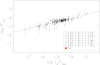 |
Fig. 1 Log |
4. Empirical and theoretical convective turnover times
4.1. Physical meaning and empirical origins of the convective turnover time
Naively one expects to find a clear correlation between the mean activity and rotation period. Yet, in their study of chromospheric emission Noyes et al. (1984) pointed out that there is no such one-to-one relationship between the (logarithm of the) index and the (logarithm of the) rotation period P. However, by considering the colour and thus mass dependent Rossby number RO, defined as the ratio of the rotation period (P) to convective turnover time (τc), i.e. RO = P/τc, Noyes et al. (1984) were able to demonstrate that the scatter in the rotation-activity relations can be significantly reduced and that the desired tight correlation between activity and rotation can indeed be produced.
Noyes et al. (1984) empirically introduced the convective turnover time τc,days, using the following representation by a function of stellar colour:
 (4)
(4)
for x > 0, and
 (5)
(5)
for x < 0, with x being defined as
 (6)
(6)
and found that the relation
 (7)
(7)
with y being defined as
 (8)
(8)
results in minimal scatter in a versus RO diagram.
In this fashion, the convective turnover time appears to provide the missing link between rotation period and activity, and its concept absorbs the colour and mass dependence to provide unique activity-rotation relations. Noyes et al. (1984) also used mixing length theory calculations in an attempt to determine the convective turnover time versus spectral type from first principles.
Inspecting Eq. (7), we note that the parameter used by Noyes et al. (1984) still includes the basal flux, hence does not vanish for a star with low activity near the basal flux level. This raises the question of what the activity-rotation relations look like at such low activity levels. An inspection of Table 1 in Noyes et al. (1984) shows that the smallest reported value of (i.e. for the star HD 13421) is ≈6 × 10⁻⁶ or y ≈ −0.205. Evaluating Eq. (7) with this value, we find a ratio of rotation period over convective turnover time (defined according to the definition by Noyes et al. 1984) of ≈2.5. Such stars at the basal flux level, thus virtually without activity, should then all have periods about ≈2.5 longer than their convective turnover time (again using the definition by Noyes et al. 1984).
Results of the convective turnover time estimation for each B–V bin.
Rutten (1987) investigated the relationship between the Ca II flux excess (which he called  ) and the rotation period in small B–V intervals and found a good correlation between these quantities. This fact was used by Stepien (1989) to empirically define a convective turnover time. However, he then rescaled his initial relation by a factor of ≈2.7 to match the convective turnover time defined by Noyes et al. (1984). Another empirically defined convective turnover time was introduced by Pizzolato et al. (2003), who used X-ray data, yet followed the same procedure as Stepien (1989). The thus determined convective turnover time was also rescaled to the convective turnover time for the Sun, which was assumed to be 12.6 days. Nevertheless, from Pizzolato et al. (2003, Figs. 10 and 11), we estimate a logarithmic shift of ≈0.8, which corresponds to a scaling factor of ≈6.3 for the scaled and unscaled determined turnover times.
A theoretical global convective turnover time was introduced by Kim & Demarque (1996), who argued that this should be considered as the true convective turnover time; the same authors denote the definition given by Noyes et al. (1984) as the local convective turnover time because for this relation only one-half of the mixing length is used. Obviously, local and global convective turnover time differ only by a factor (Kim & Demarque 1996).
This can be confirmed by comparing the theoretical values for the local and global convective turnover times computed by Landin et al. (2010). According to their calculations we find that this factor between local and global convective turnover times is, on average, ≈2.4 for ages larger than 100 Myears, where a constant age dependency may be assumed. The factor of 2.4 is very much comparable with the factor of 2.5 that we find from our above discussion of rotation periods of inactive stars and also with the factor derived above by Stepien (1989). Consequently, we may indeed assume that the aforementioned envelope of the period versus B–V distribution is given by the global convective turnover time (thereafter, referred to as convective turnover time τc).
4.2. Rotation periods of inactive stars and the global convective turnover time
4.2.1. Basal flux timescale
From the above discussion it clearly appears advantageous to use an activity measure that explicitly excludes the basal flux as does the index. Because of its definition as a purely activity related quantity, it should vanish for completely inactive stars. We are therefore led to describe the activity-rotation relationship in the form
![Mathematical equation: $$ \begin{eqnarray} \label{general_a-r-relation} \log P [{\rm day}] = \log \tau_{\rm c}(B{-}V)~[{\rm day}] + f(R^{+}_{\rm HK}), \end{eqnarray} $$](/articles/aa/full_html/2018/10/aa33498-18/aa33498-18-eq13.gif) (9)
(9)
where the quantity τc is a colour-dependent timescale interpreted – for the time being – as the rotation period of a star without any magnetic activity and  is – again for the time being – an arbitrary function, which is zero when becomes zero.
We next consider only less active stars with small flux excesses (i.e.  ) and therefore linearly approximate the function introduced in Eq. (9) through
 (10)
(10)
with some constant A, universally valid for all types of cool main-sequence stars.
Following Stepien (1989), we then subdivide our sample stars into smaller colour ranges listed in Table 1. The same table also provides the number of stars in each colour bin; we note that we use overlapping bins to ensure the availability of a sufficient number of stars in each colour bin with the consequence that our fit results are not independent. For each of the bins listed in Table 1 we then perform a linear regression via a least-squares fit between the  -values and the logarithmic rotation periods, where the slopes of these regressions are the inverse values of the slope A in Eq. (10). In Fig. 2 we plot the data and the so determined linear regressions for those B–V ranges with more than ten objeclues of A are averaged and we obtain a general slope A of −0.15 with a standard deviation of 0.02. With this slope A the logarithmic basal flux timescales τc,B–V bin(B–V) are estimated for each B–V colour bin listed in Table 1.
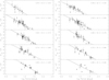 |
Fig. 2 Pure activity flux excess index |
In Fig. 3 we plot for our whole sample the measured (logarithmic) rotation periods versus B–V-colour and additionally the derived basal timescales τc,B–Vbin as listed in Table 1. We also plot the global convective turnover times for stars with an age of 4.55 Gyrs derived by (Landin et al. 2010, see Table 2) as diamonds and to guide the eye the points are connected by a dashed line; we note in this context that the global convective turnover times derived by (Landin et al. 2010, see Table 2) change only a little between ages 0.2 to 15 Gyr.
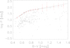 |
Fig. 3 Logarithm of the rotation periods vs. B–V. The red data points shown our τc,B−Vbin with error. The diamonds linked with a dashed line show the global convective turnover times derived by Landin et al. (2010). The black solid line shows the τc from Eqs. (11) and (12). |
Figure 3 demonstrates that, first, the colour dependent basal flux timescales τc,B–Vbin provide an upper envelope of the observed period distribution of our sample stars, and second that the global convective turnover times calculated by Landin et al. (2010) appear to agree reasonably well with this upper period envelope. We are therefore led to identify, based on this empirical result, the basal flux timescale τc,B–Vbin with the rotation periods of least active stars, and furthermore, that timescale with the global convective turnover time.
We now use this result to describe the latter empirically. For practical reasons we use a simple linear fit to our values of τc,B–Vbin and obtain our final expression for the dependence of the convective turnover time τc versus B–V-colour in the form
 (11)
for stars with colours in the range 0.44 ≤ B−V ≤ 0.71, and for stars with B−V > 0.71
(11)
for stars with colours in the range 0.44 ≤ B−V ≤ 0.71, and for stars with B−V > 0.71
 (12)
(12)
where the errors provide an estimate of the uncertainties involved. These relations are plotted as a solid line in Fig. 3.
4.2.2. Convective turnover time as upper envelope of Prot versus B–V distribution?
Recently large samples of stars with measured rotation periods have become available as a result of space-based and ground-based surveys. Specifically, McQuillan et al. (2014a) presented period measurements from high-precision Kepler data for 34030 late-type stars. In their catalogue McQuillan et al. (2014b) give Teff values rather than B − V values; to convert into B–V colours we use the Teff(B − V) relation from Gray (2005, Eq. (14.17)) and finally select 29534 stars with B–V colours between 0.4 and 1.6 and a log g value greater than 4.2. In this context, not all of the period measurements by McQuillan et al. (2014b) may necessarily refer to the stellar rotation period, however, the bulk of the period data should really provide a good measure of rotation.
Next, Newton et al. (2016a) presented rotation periods of 387 M-type stars derived from photometric MEarth observations. Since their catalogue (Newton et al. 2016b) does not provide B–V colours, we obtained the B–V colours by cross-matching this catalogue with the LSPM-North catalogue by Lepine & Shara (2005) to obtain the J−K colours, which are then transformed into B–V colours by interpolation using the colour table for solar metallicity and log g = 4.5 by Worthey & Lee (2011). Finally, we selected 314 stars satisfying B−V ≤ 1.6.
In total, we selected 29 848 stars with measured rotation periods from both catalogues and plot these periods versus the derived B–V colours in Fig. 4; we also plot our independently derived convective turnover time as a solid line; for further comparison we also plot the rescaled relations by Noyes et al. (1984), Stepien (1989), and Pizzolato et al. (2003) in Fig. 4 with a dashed line, dash-dotted line, and green triangles, respectively. The theoretical global convective turnover time for 4.55 [Gyr] by (Landin et al. 2010, see Table 2) is depicted as red diamonds in Fig. 4; since Landin et al. (2010) used log Teff, we again compute the respective B–V values using the Teff(B−V) relation from Gray (2005, Eq. (14.17)).
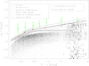 |
Fig. 4 Logarithm of the rotation periods vs. B–V from the catalogue by McQuillan et al. (2014b) and Newton et al. (2016b). Furthermore, our empirical convective turnover time calculated with Eqs. (11) and (12) is plotted as a solid line. The dotted line is labelled as the 1σ error area of convective turnover time. The rescaled relations by Noyes et al. (1984) and Stepien (1989) are plotted as dashed and dashed dotted line, respectively. The green triangle points are labelled as the values of the empirical convective turnover time by Pizzolato et al. (2003) and the values by Landin et al. (2010) are labelled with red diamonds. |
Figure 4 demonstrates that our newly derived convective turnover time also provides a good description of the upper envelope of the distribution of rotation periods of the stellar periods derived by McQuillan et al. (2014b) and Newton et al. (2016b). We therefore argue that the convective turnover time can indeed be assumed to represent an upper envelope of a period versus B–V distribution. From Fig. 4 it is easily recognized that the rescaled empirical, theoretical global, and our convective turnover time are located at the upper edge of the observed period versus B–V distribution with only small differences and therefore conclude that our assumption that the true convective turnover time is an upper envelope of the period versus B–V distribution is indeed reasonable.
4.2.3. Comparison to previously derived convective turnover times
In the following we compare our new convective turnover time with previously derived convective turnover times. Comparing the different shapes of the convective turnover times, Fig. 4 demonstrates that all relations show a strongly decreasing convective turnover time with smaller B–V values and a more or less linear behaviour at larger B–V values, yet the convective turnover times differ in their slopes for larger B–V values. The slope of the theoretical convective turnover time is slightly smaller than that of our convective turnover time, yet they still agree reasonably well. In contrast, the slopes of the relations derived by Noyes et al. (1984), Stepien (1989), and Pizzolato et al. (2003) are clearly lower, and Stepien (1989) even finds a constant convective turnover time with increasing B–V, similar to the findings of Pizzolato et al. (2003). Furthermore, we note in context that the (unscaled) convective turnover time derived by Pizzolato et al. (2003; see Fig. 10 in this paper) exceeds the corresponding estimates by Kim & Demarque (1996) by about a factor of 2; on the other hand, the estimates by Kim & Demarque (1996) and Landin et al. (2010) agree fairly well, so that the nature of this shift is entirely unclear.
The period distribution derived from the Kepler data by McQuillan et al. (2014b) shows a rather sharp edge at ≈40 days for stars with B−V > 1.0. This apparent edge lies well below our the convective turnover time, however, it is consistent with the trends of the classical rescaled relations by Noyes et al. (1984) and Stepien (1989), which result in a nearly constant or constant convective turnover time for stars B−V > 1.0. However, adding the M star data by Newton et al. (2016b), the gap between the data by McQuillan et al. (2014b) and our convective turnover time is filled up and makes the relations of Noyes et al. (1984) and Stepien (1989) inconsistent with the data.
Finally, we compare the convective turnover time of the Sun calculated with our relation with theoretical values listed in Spada et al. (2013, Fig. 16). These theoretical values of the convective turnover time for the Sun range from 31.70 days to 42.12 days; with our relation Eq. (11), we compute a convective turnover time of 33.9 ± 8.0 days, i.e. a value well in the range of the theoretical values.
4.3. Can stars rotate more slowly than their convective turnover times ?
In the previous sections we introduced the convective turnover time empirically as the upper envelope in the observed rotational period distribution of late-type stars. What remains somewhat open is why this upper envelope exists in the first place. After all, the observed rotational period distribution might be biased since it becomes increasingly difficult to measure rotation periods for less and less active stars, and there is no physical law preventing stars from braking to essentially zero rotational velocity. We, however, argue that this problem does not appear in practice. In gyrochronology the following equation is used to relate the stellar age tage with the rotation period P and the convective turnover time τ (Barnes 2010):
 (13)
where the parameters PO, kC, and kI take on the values P0 = 1.1 day, kC = 0.646 day Myr−1, and kI = 452 Myr day−1. Using Eq. (13) we can compute that age tbreak, when the rotation period P equals the convective turnover time τ, and the resulting values are shown in Fig. 5 as a function of stellar mass.
(13)
where the parameters PO, kC, and kI take on the values P0 = 1.1 day, kC = 0.646 day Myr−1, and kI = 452 Myr day−1. Using Eq. (13) we can compute that age tbreak, when the rotation period P equals the convective turnover time τ, and the resulting values are shown in Fig. 5 as a function of stellar mass.
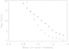 |
Fig. 5 Convective turnover time (asterisks) vs. main-sequence lifetime (diamonds) vs. stellar mass. |
These values of tbreak need to be compared to the main-sequence lifetimes tms. To estimate tms, we use the time span between a star’s arrival on the main sequence and its first turning point, i.e. the time when the hydrogen fuel becomes exhausted in the core, the star becomes redder, and starts ascending the giant branch. We use the evolutionary tracks computed and tested by Schroeder (1998) to obtain the reliable main-sequence lifetimes tms of the stars in the relevant mass range; the models specifically deal with convective overshooting and its onset at about 1.5 M⊙.
The so-computed values of tms are also shown in Fig. 5 (with diamonds). As becomes clear from Fig. 5, for stars with masses M* > 0.8 M⊙ the main-sequence lifetimes tms are always shorter than the ages tbreak. In other words, stellar evolution, which makes the stars evolve and move up the giant branch, is faster than magnetic braking, which tries to spin down the stars to their convective turnover times. For stars with masses M* < 0.8 M⊙ the main-sequence lifetimes tms exceed the ages tbreak, however, given the age of the universe, such stars have not had their chance to experience rotational braking throughout their full main-sequence careers. For such stars tbreak scales as a multiple of tms, and as already noted by Schröder et al. (2013) and consistent with the studies by Reiners & Mohanty (2012), this implies that magnetic braking scales with the relative main-sequence evolutionary age of solar-like stars of different masses. As a consequence, we infer that a complete slowdown of stellar rotation by magnetic braking seems to be impossible on the main sequence for stars like our Sun.
Yet there is an additional argument in this context. Once the Rossby number reaches the value of unity and hence any chromospheric emission is reduced to the basal flux level, there is no magnetic dynamo action with emerging active regions any more, rather only small-scale activity is expected to be present on the star. Following models of the global magnetic field of the Sun under such conditions (Meyer & Mackay 2016), we speculate that magnetic braking becomes less efficient because of the decrease of the magnetic field strength, which provides another reason why the rotation periods of basal flux stars form an envelope to the observed rotation periods.
5. Magnetic activity related Ca II H&K emission and Rossby number
5.1. versus Rossby number
The Ca II H&K excess flux is thought to be caused purely by dynamo-produced stellar magnetic activity. An important ingredient of dynamo action is of course rotation, which is directly involved in the definition of the Rossby number. The correlation between Ca II H&K excess flux and Rossby number was established long ago (e.g. Noyes et al. 1984), and the general shape of the dependence of Ca II H&K excess flux and Rossby number has been derived by previous authors (see e.g. Noyes et al. 1984, Fig. 8; Mamajek & Hillenbrand 2008, Fig. 7). However, the Rossby number definitions previously used do not constrain the Rossby number to a well-defined range. By contrast, our approach of equating global convective turnover times with the rotation periods of entirely inactive main-sequence stars leads to a well-defined Rossby number range between 0.0 and 1.0; the latter value denotes the maximal rotation period a star can have. We now address the question of which range of Ca II H&K excess flux this range of the Rossby numbers corresponds to.
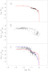 |
Fig. 7 Log |
In Fig. 6 we plot the values of Ca II H&K excess flux versus Rossby number RO computed from our empirically derived convective turnover time (cf. Eqs. (11) and (12)) for the objects listed in Table A.1. As expected, large values of go along with small values of Rossby numbers, however, we also recognize a clear change in the trend of this dependence. For fast rotators (with small RO) the excess flux decreases very fast from the saturation level to a flux level lower than  , yet the saturation level of
  and log
  , respectively, cannot be particularly well estimated from our data because we have only seven data points in range lower than RO = 0.04. Furthermore, the Rossby number, below which saturation sets in, is also not well determined from our data.
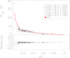 |
Fig. 6 Upper plot: Ca II H&K flux excess |
Following an initial strong decrease, the excess flux continues to decrease less steeply until a value of RO ≈ 0.28 is reached. To estimate the trend in this range we ignore those four data points with a flux excess lower than 2 because these data points are located more than 3σ below the rest and test whether a linear trend is justified; from Spearsman’s ρ we estimate the correlation coefficient and its significance, which turn out to be −0.23 with a significance of 92%. For larger values of RO, the flux decrease becomes slightly stronger and the flux excess eventually disappears with the Rossby number reaching unity; we also refer to Fig. 7 (top panel) for a double logarithmic plot of the same data.
To empirically describe the dependence of on Rossby number we therefore introduce four parameter regions and we obtain the following approximations: For the range RO < 0.021 we find
 (14)
(14)
for the range 0.021 ≤ RO < 0.14 we have
 (15)
(15)
with x = log(RO) − log(0.14), and for 0.14 ≤ RO < 0.28 we have
 (16)
(16)
with x = log(RO) − log(0.28) and finally for RO ≥ 0.28 we have
 (17)
(17)
with x = log(RO).
The relation described by Eqs. (14)–(17) is shown as a red solid line in Fig. 6. We estimate a standard deviation of ≈2.3. However, the size of the scatter is different in the different ranges. We obtain a standard deviation of the residuals of 8.8 for RO < 0.021, 3.8 for 0.024 ≤ RO < 0.14, 1.1 for 0.14 ≤ RO < 0.28, and 0.7 for RO ≥ 0.28. To test for a remaining colour dependency in the flux evolution, the data in different B–V ranges are labelled with different symbols in Fig. 6 and no colour dependence is seen.
5.2. Comparison of , Hα, and X-ray flux evolution versus Rossby number
Finally, we compared our newly derived versus Rossby number relation with the equivalent relations derived for Hα and X-ray data. For this comparison we used the LHα/Lbol-values derived by Newton et al. (2017) for a sample of M dwarfs and the LX/Lbol values derived by Wright et al. (2011) for a sample of late-type stars; in all cases we only used stars with measured rotation periods.
We calculated the Rossby numbers for the selected sample objects with our new empirical convective turnover time. In both catalogues, no B–V-values are provided. For the objects studied by Newton et al. (2017), we used the same method as described in Sect. 4.2.2. The catalogue by Wright et al. (2011) provides effective temperatures for all entries, which we transform into the B–V colour using the Teff(B−V) relation from Gray (2005, Eq. (14.17)). In Fig. 7 we plot the dependence of these three activity indicators versus Rossby number. Clearly, the general shape of the relation is the same in all three indicators, yet some differences are discernible. The saturation level in the values and the log LHα/Lbol values is comparable, considering the fact that we have only very few data points at the saturation level, while the saturation level of the log LX/Lbol data is higher than that of the values.
To compare the Rossby number dependence of the various activity indicators we plot our flux trend Eqs. (14)–(17) into Fig. 7 as a red line. As is clear from Fig. 7, the Hα data show a large scatter for data with Rossby numbers larger 0.1, which makes a comparison difficult. Therefore, we can only say that the log LHα/Lbol dependence on Rossby number is described in general; there is a possible overprediction in the saturation region. As far as the X-ray data are concerned, it is clear that the flux trend of Eqs. (14)–(17) does not fit the data particularly well. However, using the transformation relation between log and log LX/Lbol derived in Sect. 3.2, we can rescale the activity-Rossby number relation and arrive at the blue line in the Fig. 7(c), which describes the log LX/Lbol versus Rossby number relation very well, except in the saturation region, which lies clearly above the observed X-ray saturation. We therefore suspect that our saturation level could be too high, possibly as a consequence of the low number of data points to estimate the saturation level in the Ca II data.
6. Summary and conclusions
In this paper we revisit the connection between the purely magnetic activity related Ca II H&K flux excess and the rotation period for main-sequence stars, focussing on the index. This index is determined by first subtracting all non-magnetic activity contributions from the Ca II H&K line core flux, notably the photospheric flux and basal chromospheric flux, and second normalizing by the bolometric flux. By contrast, the older activity index still includes the basal chromospheric flux and therefore contains contributions not directly attributable to the effects of magnetic activity. We demonstrate that the index provides a very good physical representation of the stellar chromospheric activity, since it relates very well with the coronal X-ray flux, using the LX/Lbol data for a sample of stars with measured S-indices, X-ray fluxes, and rotation periods.
Revisiting the rotation-activity relation with our new indicator we find that the chromospheric flux reaches zero for inactive (basal flux) stars, which have a well-defined colour dependent rotation period. This result is intuitively consistent with the idea that in an inactive star no significant magnetic braking can take place any further, which forces it to maintain its rotational angular momentum from that point in its evolution, until substantial mass loss sets in. These resulting basal flux rotation periods only depend on the B–V colour and compare to the data in the same way as earlier empirical concepts of convective turnover time.
We show that this convective turnover time provides a very good representation of the upper envelope of the observed period versus B–V distribution for a very large sample of cool stars and then, using both by empirical and theoretical approaches, we compare the resulting convective turnover times with previous prescriptions. Our approach turns out to be fully consistent with the theoretical relation proposed by Landin et al. (2010), but we find significant differences between our relation and those derived by Noyes et al. (1984), Stepien (1989), and Pizzolato et al. (2003), especially in the slope in the range B−V > ≈0.9.
We emphasize that with this new definition of the convective turnover time, the Rossby number (for main-sequence stars) has a well-defined definition range from zero to unity. When the relation of these new Rossby numbers with the Ca II H&K flux excess is investigated, a clear evolutionary picture emerges, dividing this relation into distinct parts: for small values of the Rossby number (fast rotating star with large activity) the excess flux is saturated. Then it initially decreases quickly and then more slowly, thus asymptotically reaching zero, where the Rossby number has reached unity. A good example is the well-known planet host 51 Peg (HD 217014), which is a somewhat evolved main-sequence stars (Mittag et al. 2016) with a low SMWO value of 0.149, very close to the basal S-index level of 0.144 (Mittag et al. 2013). With our new convective turnover time the Rossby number of 51 Peg is 0.96 ± 0.24, i.e. very close to unity and therefore its rotation period of 37 days (Wright et al. 2011) should essentially comparable with the basal flux timescale of 38.6 days computed with Eq. (11).
Finally, we compare the estimated trend of versus Rossby number with LHα/Lbol and LX/Lbol data versus Rossby number and find that the general trend is the same in all three activity indices. Furthermore, plotting our flux trend into the good match of the data is obtained especially with the X-ray data after the adjustment of the trend at the X-ray data with the transformation equation, which suggests a universality of the Rossby number activity relations.
Acknowledgments
This research has made use of the VizieR catalogue access tool, CDS, Strasbourg, France. The original description of the VizieR service was published in A & AS, 143, 23.
Appendix A: Additional table
Objects used with the corresponding B−V colour index, S-values, rotational period, and log LX/Lbol.
References
- Baliunas, S. L., Donahue, R. A., Soon, W. H., et al. 1995, ApJ, 438, 269 [NASA ADS] [CrossRef] [Google Scholar]
- Baliunas, S. L., Donahue, R. A., Soon, W., & Henry, G. W. 1998, in Cool Stars, Stellar Systems, and the Sun, eds. R. A. Donahue, & J. A. Bookbinder, ASP Conf. Ser., 154, 153 [NASA ADS] [Google Scholar]
- Barnes, S. A. 2010, ApJ, 722, 222 [NASA ADS] [CrossRef] [Google Scholar]
- Cayrel de Strobel, G. 1996, A&AR, 7, 243 [CrossRef] [Google Scholar]
- Cincunegui, C., & Mauas, P. J. D. 2003, VizieR Online Data Catalog: J/A+A/341/699 [Google Scholar]
- Dobson, A. K. 1992, in Cool Stars, Stellar Systems, and the Sun, eds. M. S. Giampapa, & J. A. Bookbinder, ASP Conf. Ser., 26, 297 [NASA ADS] [Google Scholar]
- Donahue, R. A. 1998, in Cool Stars, Stellar Systems, and the Sun, eds. R. A. Donahue, & J. A. Bookbinder, ASP Conf. Ser., 154, 1235 [NASA ADS] [Google Scholar]
- Duncan, D. K., Vaughan, A. H., Wilson, O. C., et al. 2005, VizieR Online Data Catalog: III/159 [Google Scholar]
- ESA (ed.) 1997, The HIPPARCOS and TYCHO catalogues. Astrometric and Photometric Star Catalogues Derived From the ESA HIPPARCOS Space Astrometry Mission, ESA SP, 1200 [Google Scholar]
- Gray, D. F. 2005, The Observation and Analysis of Stellar Photospheres (Cambridge, UK: Cambridge University Press) [CrossRef] [Google Scholar]
- Gray, R. O., Corbally, C. J., Garrison, R. F., McFadden, M. T., & Robinson, P. E. 2003, AJ, 126, 2048 [NASA ADS] [CrossRef] [Google Scholar]
- Gray, R. O., Corbally, C. J., Garrison, R. F., et al. 2006, AJ, 132, 161 [NASA ADS] [CrossRef] [Google Scholar]
- Hauschildt, P. H., Allard, F., & Baron, E. 1999, ApJ, 512, 377 [NASA ADS] [CrossRef] [Google Scholar]
- Hempelmann, A., Robrade, J., Schmitt, J. H. M. M., et al. 2006, A&A, 460, 261 [NASA ADS] [CrossRef] [EDP Sciences] [Google Scholar]
- Henry, T. J., Soderblom, D. R., Donahue, R. A., & Baliunas, S. L. 1996, AJ, 111, 439 [NASA ADS] [CrossRef] [Google Scholar]
- Henry, G. W., Baliunas, S. L., Donahue, R. A., Fekel, F. C., & Soon, W. 2000, ApJ, 531, 415 [NASA ADS] [CrossRef] [Google Scholar]
- Howard, A. W., Marcy, G. W., Fischer, D. A., et al. 2014, ApJ, 794, 51 [Google Scholar]
- Isaacson, H., & Fischer, D. 2010, ApJ, 725, 875 [NASA ADS] [CrossRef] [Google Scholar]
- Kim, Y.-C., & Demarque, P. 1996, ApJ, 457, 340 [NASA ADS] [CrossRef] [Google Scholar]
- Landin, N. R., Mendes, L. T. S., & Vaz, L. P. R. 2010, A&A, 510, A46 [NASA ADS] [CrossRef] [EDP Sciences] [Google Scholar]
- Lepine, S., & Shara, M. M. 2005, VizieR Online Data Catalog: I/298 [Google Scholar]
- Linsky, J. L., McClintock, W., Robertson, R. M., & Worden, S. P. 1979, ApJS, 41, 47 [NASA ADS] [CrossRef] [Google Scholar]
- Maggio, A., Sciortino, S., Vaiana, G. S., et al. 1987, ApJ, 315, 687 [NASA ADS] [CrossRef] [Google Scholar]
- Mamajek, E. E., & Hillenbrand, L. A. 2008, ApJ, 687, 1264 [NASA ADS] [CrossRef] [Google Scholar]
- McQuillan, A., Mazeh, T., & Aigrain, S. 2014a ApJS, 211, 24 [NASA ADS] [CrossRef] [MathSciNet] [Google Scholar]
- McQuillan, A., Mazeh, T., & Aigrain, S. 2014b, VizieR Online Data Catalog: J/ApJS/211/24 [Google Scholar]
- Meyer, K. A., & Mackay, D. H. 2016, ApJ, 830, 160 [NASA ADS] [CrossRef] [Google Scholar]
- Middelkoop, F. 1982, A&A, 107, 31 [NASA ADS] [Google Scholar]
- Mittag, M., Schmitt, J. H. M. M., & Schröder, K.-P. 2013, A&A, 549, A117 [NASA ADS] [CrossRef] [EDP Sciences] [Google Scholar]
- Mittag, M., Schröder, K.-P., Hempelmann, A., González-Pérez, J. N., & Schmitt, J. H. M. M. 2016, A&A, 591, A89 [NASA ADS] [CrossRef] [EDP Sciences] [Google Scholar]
- Mittag, M., Hempelmann, A., Schmitt, J. H. M. M., et al. 2017a, A&A, 607, A87 [NASA ADS] [CrossRef] [EDP Sciences] [Google Scholar]
- Mittag, M., Robrade, J., Schmitt, J. H. M. M., et al. 2017b, A&A, 600, A119 [NASA ADS] [CrossRef] [EDP Sciences] [Google Scholar]
- Newton, E. R., Irwin, J., Charbonneau, D., et al. 2016a, ApJ, 821, 93 [NASA ADS] [CrossRef] [Google Scholar]
- Newton, E. R., Irwin, J., Charbonneau, D., et al. 2016b, VizieR Online Data Catalog: J/ApJ/821/93 [Google Scholar]
- Newton, E. R., Irwin, J., Charbonneau, D., et al. 2017, VizieR Online Data Catalog: J/ApJ/834/85 [Google Scholar]
- Noyes, R. W., Hartmann, L. W., Baliunas, S. L., Duncan, D. K., & Vaughan, A. H. 1984, ApJ, 279, 763 [NASA ADS] [CrossRef] [Google Scholar]
- Pizzolato, N., Maggio, A., Micela, G., Sciortino, S., & Ventura, P. 2003, A&A, 397, 147 [NASA ADS] [CrossRef] [EDP Sciences] [Google Scholar]
- Reiners, A., & Mohanty, S. 2012, ApJ, 746, 43 [NASA ADS] [CrossRef] [Google Scholar]
- Rutten, R. G. M. 1984, A&A, 130, 353 [NASA ADS] [Google Scholar]
- Rutten, R. G. M. 1987, A&A, 177, 131 [NASA ADS] [Google Scholar]
- Schrijver, C. J. 1987, A&A, 172, 111 [NASA ADS] [Google Scholar]
- Schrijver, C. J., Dobson, A. K., & Radick, R. R. 1992, A&A, 258, 432 [NASA ADS] [Google Scholar]
- Schroeder, K.-P. 1998, A&A, 334, 901 [NASA ADS] [Google Scholar]
- Schroeder, C., Reiners, A., & Schmitt, J. H. M. M. 2008, VizieR Online Data Catalog: J/A+A/349/099 [Google Scholar]
- Schröder, K.-P., Mittag, M., Hempelmann, A., González-Pérez, J. N., & Schmitt, J. H. M. M. 2013, A&A, 554, A50 [NASA ADS] [CrossRef] [EDP Sciences] [Google Scholar]
- Skumanich, A. 1972, ApJ, 171, 565 [NASA ADS] [CrossRef] [Google Scholar]
- Spada, F., Demarque, P., Kim, Y.-C., & Sills, A. 2013, ApJ, 776, 87 [NASA ADS] [CrossRef] [Google Scholar]
- Stepien, K. 1989, A&A, 210, 273 [NASA ADS] [Google Scholar]
- Vaughan, A. H., Preston, G. W., & Wilson, O. C. 1978, PASP, 90, 267 [NASA ADS] [CrossRef] [Google Scholar]
- White, R. J., Gabor, J. M., & Hillenbrand, L. A. 2007, AJ, 133, 2524 [NASA ADS] [CrossRef] [Google Scholar]
- Wilson, O. C. 1963, ApJ, 138, 832 [NASA ADS] [CrossRef] [Google Scholar]
- Worthey, G., & Lee, H.-c. 2011, ApJS, 193 [Google Scholar]
- Wright, J. T., Marcy, G. W., Butler, R. P., & Vogt, S. S. 2004, VizieR Online Data Catalog: J/A+A/215/261 [Google Scholar]
- Wright, N. J., Drake, J. J., Mamajek, E. E., & Henry, G. W. 2011, ApJ, 743, 48 [NASA ADS] [CrossRef] [Google Scholar]
All Tables
Objects used with the corresponding B−V colour index, S-values, rotational period, and log LX/Lbol.
All Figures
|
Fig. 1 Log |
| In the text | |
|
Fig. 2 Pure activity flux excess index |
| In the text | |
|
Fig. 3 Logarithm of the rotation periods vs. B–V. The red data points shown our τc,B−Vbin with error. The diamonds linked with a dashed line show the global convective turnover times derived by Landin et al. (2010). The black solid line shows the τc from Eqs. (11) and (12). |
| In the text | |
|
Fig. 4 Logarithm of the rotation periods vs. B–V from the catalogue by McQuillan et al. (2014b) and Newton et al. (2016b). Furthermore, our empirical convective turnover time calculated with Eqs. (11) and (12) is plotted as a solid line. The dotted line is labelled as the 1σ error area of convective turnover time. The rescaled relations by Noyes et al. (1984) and Stepien (1989) are plotted as dashed and dashed dotted line, respectively. The green triangle points are labelled as the values of the empirical convective turnover time by Pizzolato et al. (2003) and the values by Landin et al. (2010) are labelled with red diamonds. |
| In the text | |
|
Fig. 5 Convective turnover time (asterisks) vs. main-sequence lifetime (diamonds) vs. stellar mass. |
| In the text | |
|
Fig. 7 Log |
| In the text | |
|
Fig. 6 Upper plot: Ca II H&K flux excess |
| In the text | |
Current usage metrics show cumulative count of Article Views (full-text article views including HTML views, PDF and ePub downloads, according to the available data) and Abstracts Views on Vision4Press platform.
Data correspond to usage on the plateform after 2015. The current usage metrics is available 48-96 hours after online publication and is updated daily on week days.
Initial download of the metrics may take a while.