| Issue |
A&A
Volume 617, September 2018
|
|
|---|---|---|
| Article Number | A115 | |
| Number of page(s) | 13 | |
| Section | Stellar structure and evolution | |
| DOI | https://doi.org/10.1051/0004-6361/201731794 | |
| Published online | 27 September 2018 | |
Catching a star before explosion: the luminous blue variable progenitor of SN 2015bh
School of Physics, Trinity College Dublin, University of Dublin,
Dublin,
Ireland
e-mail: boiani@tcd.ie; jose.groh@tcd.ie
Received:
17
August
2017
Accepted:
7
May
2018
In this paper we analyse the pre-explosion spectrum of SN2015bh by performing radiative transfer simulations using the CMFGEN code. This object has attracted significant attention due to its remarkable similarity to SN2009ip in both its pre- and post-explosion behaviour. They seem to belong to a class of events for which the fate as a genuine core-collapse supernova or a non-terminal explosion is still under debate. Our CMFGEN models suggest that the progenitor of SN2015bh had an effective temperature between 8700 and 10 000 K, had a luminosity in the range ≃1.8−4.74 × 10⁶ L⊙, contained at least 25% H in mass at the surface, and had half-solar Fe abundances. The results also show that the progenitor of SN2015bh generated an extended wind with a mass-loss rate of ≃6 × 10⁻⁴ to 1.5 × 10⁻³ M⊙ yr−1 and a velocity of 1000km s−1. We determined that the wind extended to at least 2.57 × 1014 cm and lasted for at least 30 days prior to the observations, releasing 5 × 10⁻⁵ M⊙ into the circumstellar medium. In analogy to 2009ip, we propose that this is the material that the explosive ejecta could interact at late epochs, perhaps producing observable signatures that can be probed with future observations. We conclude that the progenitor of SN2015bh was most likely a warm luminous blue variable of at least 35 M⊙ before the explosion. Considering the high wind velocity, we cannot exclude the possibility that the progenitor was a Wolf–Rayet (WR) star that inflated just before the 2013 eruption, similar to HD5980 during its 1994 episode. If the star survived, late-time spectroscopy may reveal either a similar luminous blue variable (LBV) or a WR star, depending on the mass of the H envelope before the explosion. If the star exploded as a genuine supernova (SN), 2015bh would be a remarkable case of a successful explosion after black hole formation in a star with a possible minimum mass 35 M⊙ at the pre-SN stage.
Key words: supernovae: general / stars: evolution / supernovae: individual: SN2015bh / supernovae: individual: SN2009ip / stars: massive
© ESO 2018
1 Introduction
Stars more massive than 8 M⊙ end their lives in violent events called core-collapse supernovae (SNe). While SN explosions and their feedback are related to a multitude of topics in astrophysics, the link between SNe and their progenitor stars is still not fully understood.
Massive stars eject large quantities of material into the interstellar medium throughout their evolution and before explosion (de Jager et al. 1988; Maeder & Meynet 2000; Langer 2012; Kiewe et al. 2012; Smith 2014; Groh et al. 2014). Some stars undergo increased instabilities before death, leading to sudden and massive material ejections on short timescales of a few days to decades, as shown, for example, by SN1988Z (Stathakis & Sadler 1991; Turatto et al. 1993), SN1994W (Sollerman et al. 1998; Chugai et al. 2004), SN1998S (Leonard et al. 2000; Fassia et al. 2001), SN2005gj (Trundle et al. 2008), SN 2005gl (Gal-Yam et al. 2007; Gal-Yam & Leonard 2009), and SN2006gy (Smith et al. 2007). This material builds up around the star forming a circumstellar medium (CSM). The SN ejecta crashes into this medium and the kinetic energy of this interaction is partially converted into radiation. Depending on the CSM density, the interaction can give rise to luminous transients comparable to the luminosities of the actual SN (e.g. Chevalier & Fransson 1994). Due to the radiation originating in the slow-moving CSM (typically 100−1000km s−1), the spectra of these events are characterised by relatively narrow emission lines (Chugai 2001; Dessart et al. 2009, 2015). These explosions, known as interacting SNe or SN IIn (Schlegel 1990), can be used to probe the circumstellar material and constrain the properties of the progenitor, including abundances, mass-loss rate, wind velocity, and radius (Groh 2014; Gräfener & Vink 2016).
Depending on the density and extension of the CSM, the progenitor properties can be directly retrieved from follow-up spectroscopic observations obtained from a few hours up to decades after the explosion. For example, SN2013fs shows signatures of CSM interaction for the first two days and afterwards it behaves as a regular SN IIP (Yaron et al. 2017). In contrast, the interaction can last for many years when the material around the star is dense and extended, as in the case of SN 1998S (Mauerhan & Smith 2012; Shivvers et al. 2015). There is mounting evidence of SNe that are intermediate to compact, relatively low-density CSMs of SN IIP and extended, dense CSM of SN IIn. Examples of intermediate SNe are SN 2013cu (IIb; Gal-Yam et al. 2014; Groh 2014) and iPTF13iqb (Smith et al. 2015).
For some events, the continuing interaction makes it difficult to determine whether it is a genuine SN that interacts with a pre-existing CSM or if the star survived after a series of massive eruptions, in which case it is deemed a SN impostor (e.g. Van Dyk et al. 2000). One of the best observed transients whose fate is under discussion is SN2009ip, which has been monitored photometrically and spectroscopically with exquisite time coverage (Fraser et al. 2013; Mauerhan et al. 2013; Ofek et al. 2013; Pastorello et al. 2013; Prieto et al. 2013; Levesque et al. 2014; Margutti et al. 2014; Smith et al. 2014). The spectrum, energetics, low Ni mass, and late time evolution resemble both scenarios, SN and SN impostor, with Graham et al. (2017), Smith et al. (2014), Ofek et al. (2013), and Mauerhan et al. (2013) favouring the core-collapse case, while Fraser et al. (2015) states that there is no conclusive evidence for it. Moriya (2015) proposed a two-component medium, an inner shell and an outer wind. Inside this medium, an explosion took place and the material crashed into the inner shell creating the apparent SN. The slow decay is maintained by the continuous interaction with the outer wind. The explosion properties estimated by Moriya (2015) point to either a SN impostor or a peculiar SN. SN2009ip is still showing signs of interaction, masking the remnant of the event, if any.
Recent studies suggest that several other events are similar to 2009ip, forming a distinct class of transients (Elias-Rosa et al. 2016; Thöne et al. 2017; Pastorello et al. 2018). Among these, SN2015bh bears a remarkable resemblanceto SN2009ip, as discussed extensively in Thöne et al. (2017), Elias-Rosa et al. (2016), Pastorello et al. (2018), and has a unique pre-explosion spectrum observed at the lowest ever flux level for this class of transients. SN2015bh, also known as SNhunt275 or PTF13efv, was first officially reported as a SN candidate in February 2015 (Elias-Rosa et al. 2015), due to a brightening event dubbed 2015A that peaked at an absolute magnitude of MR = −15 mag. This was the first of two light curve peaks, with the second peak, now labelled 2015B, reaching MR = −17.5 mag on May 2015.
There is a significant amount of information on the precursor of SN2015bh. Its host galaxy was monitored for 21 yr before the discovery of SN2015bh, which provided extended photometric data of the progenitor. This revealed a long-term photometric variation of ± 2 mag sometimes showing sudden changes in brightness in 2008, 2009, and 2013 (Thöne et al. 2017). Serendipitous spectroscopy of the progenitor of SN2015bh was obtained on 12 November 2013, when its absolute magnitude was MR ~−10.5 mag. Although the star has documented variability, at this point the spectrum does not show any signs of interaction. This spectrum is characterised by H and Fe II emission (Thöne et al. 2017), and is one of the first times that a spectrum of a potential SN progenitor has been observed. Therefore, these observations reveal invaluable information on massive stars and their pre-SN behaviour. The 12 November 2013 observations were taken right at the onset of another eruption, detected in December 2013 by iPTF (Ofek et al. 2016). The first iPTF photometric detection of this outburst was on 26 November 2013, but Ofek et al. (2016) mention the possibility that it had started at an earlier date. After the December 2013 event, SN2015bh shows another sudden increase in brightness of 2 mag. The light curve of SN2015bh is discussed in detail in both Thöne et al. (2017) and Elias-Rosa et al. (2016).
Ofek et al. (2016) analyse the pre-explosion spectrum of SN2015bh obtained during the December 2013 outburst. The spectrum exhibits a strong, narrow Hα line with a P Cygni absorption component extending up to − 1300km s−1. By fitting a black body to the continuum, Ofek et al. (2016) obtained an effective temperature of 5750 K and a radius of 4 × 1014 cm. Assuming a super-Eddington continuum-driven wind, they estimated the total mass lost during the December 2013 event to be M ≃ 4 × 10⁻⁵M⊙. Thöneet al. (2017) analyse both the pre- and post-explosion observations, proposing that SN2015bh was a luminous blue variable (LBV) star in outburst for over 20 yr that experienced a possible SN explosion (2015B) after several precursor events. They also entertain the possibility of the star surviving and becoming a WR star and, given the similarities to a number of other events (SN2009ip, SNhunt248, and SN1961V) they propose the existence of a new category of transients. The members of this category show variations of ≃ 2 mag for at least a few decades, a bright precursor rapidly followed by a main event resembling a SN, and LBV-type spectra during the outbursts and until after the maximum of the main event. Elias-Rosa et al. (2016) also propose that SN2015bh was a massive blue star. However, they argue that the SN explosion was actually the 2015 A event, explaining that the low luminosity was due to massive fallback of material onto a collapsed core. They further suggest that the 2015B event was the result of the SN ejecta interacting with a dense CSM, but do not completely rule out a non-terminal explosion.
SN2015bh offers the unique opportunity of investigating the pre-SN spectrum of a massive star before explosion. This paper is organised as follows. In Sect. 2, we present the characteristics of CMFGEN, the code that was used to model the spectrum of the SN2015bh progenitor. Section 3 provides a detailed discussion of the results obtained from our models, while Sect. 4 puts the results in the context of other SNe, SN impostors, and other similar events. The main points of the paper are summarised in Sect. 5.
2 Radiative transfer modelling
We investigate the properties of the SN2015bh progenitor by computing radiative transfer models of the outflow produced by the star. We fit the spectrum obtained on 12 November 2013 by Thöne et al. (2017) with the Gran Telescopio Canarias (GTC) and downloaded via the WISeREP1 repository (Yaron & Gal-Yam 2012). We employ the line-blanketed atmospheric/wind radiative transfer code CMFGEN (Hillier & Miller 1998). The code computes continuum and line formation in non-local thermodynamic equilibrium and spherical symmetry, and it does not account for time-dependent effects. Including clumping effects in the winds of massive stars has improved the modelling ofspectral observations in many cases, such as Eta Car (Hillier et al. 2001; Groh et al. 2012), AG Car (Groh et al. 2009b), and the Pistol Star and FMM362 (Najarro et al. 2009). Our models include clumping with a volume filling factor of f = 0.1; we explore the effects of clumping in Sect. 3.3.
The input physical quantities that the code requires to compute the spectrum are the inner boundary radius (R⋆), a constant mass-loss rate (Ṁ), the wind terminal velocity (v∞), abundances, and the bolometric luminosity (L⋆). CMFGEN does not solve for a self-consistent hydrodynamical solution for the outflow. Instead we assume a density scale height for the atmosphere of the star of 0.02 R⋆ joined smoothly to the wind just below the sonic point (at v = 8km s−1). The stationary wind has a density profile derived from the mass continuity equation
 (1)
(1)
and accelerates following a beta-type law
![\begin{equation*} v(r)=\frac{v_0+(v_{\infty}-v_{0})(1-R_{\star}/r)^{\beta}}{(1+v_0/{v_{\textrm{core}}} \exp{([R_{\star}-r]/h_{\mathrm{eff}})}}, \end{equation*}](/articles/aa/full_html/2018/09/aa31794-17/aa31794-17-eq2.png) (2)
(2)
where vo is the velocity at a reference radius close to R⋆, vcore is the velocity at the inner radius R⋆, v∞ is the terminal velocity of the wind, and heff is the scale height in units of R⋆. Our models assume v0 = 10km s−1, vcore = 0.85km s−1, heff = 0.02R⋆, and β = 2.5. The β parameter describes the steepness of the velocity law and we have chosen a value typical of LBVs. For example, other similar works that have led to this β value for LBVs include Najarro et al. (1997), Najarro (2001) for P Cygni, Najarro et al. (2009) for the Pistol Star, and Hillier et al. (1998) for HDE 316285. We discuss the effects of β in Sect. 3.3. Figure 1 shows the velocity, density, and optical depth structures of the SN 2015bh progenitor.
We assume diffusion approximation at the inner boundary and adjust vcore to obtain a Rosseland optical depth of τRoss = 150 at R⋆. Because the2015bh progenitor has a dense wind, the photosphere is located in the wind. Hereafter, we define Teff as the effective temperature computed atthe radius where τRoss = 2/3, and likewise T⋆ at τRoss = 20. The outer boundary is defined at Rout = 250 R⋆ and is chosen to be large enough to account for all the emission line region. The region between R⋆ and Rout is split into 77 depth points where we calculate the values of each physical quantity necessary to simultaneously solve for the energy level populations and the properties of the radiation field. The atoms included in the model are summarised in Table 1, together with the number of “super” levels2 used and the number of atomic levels. Our models account for the effects of charge-exchange reactions. In the context of this paper, one reaction of major importance for the Fe II spectrum is Fe2+ + H ↔ Fe+ + H+ (Hillier et al. 2001) since it affects the Fe ionisation structure. The atomic data is provided by a number of sources, as described in detail in Hillier & Miller (1998).
After computing the atmospheric and wind structure, we use CMF_FLUX (Busche & Hillier 2005) to calculate the synthetic spectrum in the observer’s frame. We determine the properties of the SN2015bh progenitor mainly by comparing the observed optical spectrum (4000−6700Å) to the synthetic spectrum generated from our models. While the original model spectra has an arbitrarily high spectral resolution, we use a degraded version by convolving the original model spectrum with a Gaussian function with full width at half maximum FWHM = 300km s−1 to better match the spectral resolution of the observations. Fitting the strength of the emission lines to the ones in the observed spectrum, we were able to constrain Ṁ and Teff indirectly by modifying R⋆ and L⋆, and the metallicity Z. Then we matched the width of the emission lines to obtain a good approximation for v∞. The value of L⋆ is constrained by comparing the observed flux to our model and accounting for interstellar extinction using the reddening law from Fitzpatrick (1999). Thöne et al. (2017) quote a distance of d = 27 Mpc to the host galaxy, while Elias-Rosa et al. (2016) derived d = 29.3 ± 2.1 Mpc from the recessional velocity of the galaxy. We have added the distance uncertainty to our luminosity calculations. Following this procedure, we found a best-fit model that reproduces the observed properties reasonably well and is discussed in detail in the next section.
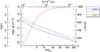 |
Fig. 1 Velocity (red), density (blue), and Rosseland optical depth structures (green) for the 2015bh progenitor based on the CMFGEN modelling of the 12 November 2013 spectrum. |
Atomic model used in the CMFGEN analysis of 2015bh.
3 Results
3.1 Physical properties of the SN2015bh progenitor
The SN2015bh spectrum taken on 12 November 2013 shows strong H I λ6363 Å emission; a multitude ofFe II λλ4924, 5018, 5196, 5198, 5235, 5276, 5317 Å lines; and a Na I λ5889 Å line. All the lines have P Cygni profiles. Figure 2 shows the observed normalised 2013 spectrum of SN2015bh (grey) and the normalised synthetic spectrum from one of our best-fitting models (red) at optical wavelengths. Our models reproduce the strength of the Hα line reasonably well (Fig. 2c), but it slightly overestimates the H β emission (Fig. 2b). This could be due to the ionisation and/or density structures not being fully reproduced by our models. In a similar manner, most Fe II lines are well fitted, but two of them are overestimated (Fe II λ5169 Å and Fe II λ5317 Å). A summary of the physical properties of the progenitor of SN2015bh is presented in Table 2.
We can constrain Ṁ and T⋆ by fitting the strength of the H I and Fe II lines. For the model in Fig. 2, we have Ṁ =10−3 M⊙ yr−1 and T⋆ =15 000 K. Because of the high wind density, the optical depth towards the hydrostatic layers of the star is ≫ 1. The photosphere is extended and formed within moving layers, in a similar way to other LBVs such as AG Car (Groh et al. 2009b, 2011), HR Car (Groh et al. 2009a), P Cygni (Najarro et al. 1997; Najarro 2001), and Eta Car (Hillier et al. 2001; Groh et al. 2012). This causes Teff to be lower than T⋆ (see discussion in Groh et al. 2009b), and our CMFGEN model shown in Fig. 2 has Teff = 8700 K. Other combinations of Ṁ and T⋆ would also fit due to degeneracy, which is further analysed in Sect. 3.3. Table 2 lists the ranges of possible values for the parameters of the SN2015bh progenitor.
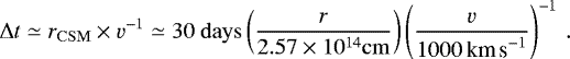
Figure 3 displays the flux-calibrated observed spectrum of SN2015bh in 12 November 2013 and one of our best-fit models, assuming RV = 3.1 and d = 27 Mpc. By comparing the absolute flux levels, we are able the constrain L⋆ and the color excess E(B − V). Under these assumptions, our CMFGEN models indicate that the bolometric luminosity of SN2015bh on 12 November 2013 is L⋆ = 2.7 × 10⁶ L⊙ and E(B − V) = 0.25. The colour excess is in remarkable agreement with the value estimated by Thöne et al. (2017) based on the strength of interstellar Na lines (E(B − V) = 0.21). However, we were also able to fit the optical spectrum using other values of RV between 2 and 5. The differences in RV have more influence at smaller wavelengths; therefore, we would like to stress the importance of multi-wavelength observations for future events. Taking into consideration the uncertainties in RV and d, the L⋆ ranges from 1.8 × 10⁶ L⊙ 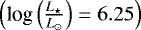 for the lowest values of RV and d, to 4.74× 10⁶ L⊙
 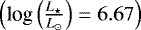 for the highest values of RV and d.
The morphology and width of the lines allowed us to determine v∞, which we have estimated to be ≃ 1000km s−1. The line profiles also show an asymmetric bump on the left side of the H β and Hβ lines. This could indicate a higher wind velocity; we discuss the various possibilities in Sect. 3.3.
We have used the strength of the Fe II lines to determine the Fe abundance of the SN2015bh progenitor. Our models indicate the progenitor star had about half-solar Fe abundance. It is interesting to contrast the Fe abundance of SN2015bh to the O abundance of the surrounding regions of SN2015bh. Thöne et al. (2017) suggest that the O abundance of the surrounding regions is half-solar. In principle, there is no reason to expect that the progenitor of SN2015bh will have the same O abundance as that of its environment. In particular for LBVs, the O abundance is expected to be severely affected by the presence of CNO-burning products at the surface (Groh et al. 2009b, 2014). Unfortunately, the progenitor spectrum analysed here does not show any strong emission of CNO lines, and therefore the abundance of these elements cannot be constrained using solely the 12 November 2013 spectrum.
The model discussed in this section has X = 0.49 for H and Y = 0.50 for He. However, we have found that, for different values of Ṁ and T⋆, we can still reasonably fit the observed spectrum for H abundances in the range X = 0.25–0.75. A similar degeneracy has been found for other LBVs, such as HDE 316285 (Hillier et al. 1998). Throughout the range of parameters of our models, the Na I λ5889 Å line showed the weakest dependence on Ṁ and T⋆. However, the morphology of the Na I λ5889 Å line is affected by He I λ5875 Å emission, which appears when the model has low Ṁ or high T⋆.
We can estimate a lower limit for the mass of the progenitor given the luminosity obtained from the modelling. By assuming that the star is at the Eddington limit, we have L⋆ = LEDD. The relation between LEDD and the mass required for stability is
![\begin{equation*} L_{\mathrm{EDD}} = 3.22 \times 10^4 \left[ \frac{\mathrm{N(H)/N(He)}+4}{\mathrm{N(H)/N(He)}+2} \right] \left( \frac{M}{{{M}_{\odot}}} \right) {{L}_{\odot}}\,. \end{equation*}](/articles/aa/full_html/2018/09/aa31794-17/aa31794-17-eq5.png) (3)
(3)
Considering the assumptions discussed previously, our best-fit model indicates that L⋆ = 2.7 × 10⁶L⊙ and that N(H)∕N(He) = 3.846; therefore, the minimum mass of the progenitor of SN2015bh at the pre-explosion stage is Mmin ≃ 62 M⊙. However, taking into account the H abundance and the L⋆ uncertainties, the minimum mass range changes significantly, giving Mmin = 35−120 M⊙.
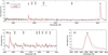 |
Fig. 2 Panel a: optical spectrum of one of our best-fitting models (red) compared to the observed spectrum taken on 12 November 2013 (grey) in the 4300–6700 Å region; see text for model parameters. Panel b: zoom-in from 4800 to 5400 Å, containing the Hβ line and a forest of Fe II lines. Panel c: zoom-in around the Hα line. |
CMFGEN model parameter ranges for the best-fitting models of the SN2015bh progenitor.
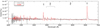 |
Fig. 3 Flux-calibrated spectrum of SN2015bh observed on 12 November 2013 (grey) compared to one of our best-fit CMFGEN models (red). This model has been scaled to a distance of d = 27 Mpc and reddened using E(B − V) = 0.25 and RV= 3.1. |
3.2 CSM properties
Based on our CMFGEN models, we can infer lower limits for the properties of the CSM surrounding the progenitor of SN2015bh, such as its extent and mass, and the duration of the stellar wind ejection required to give the November 2013 spectrum.
CSM extension. CMFGEN is able to compute the regions where the spectral lines are formed, which allows us to estimate how extended the CSM is. For this purpose we use the Hα line; we predict that this line forms over the largest distance from the star (Fig. 4). The extension of the H β emitting region is estimated as rCSM = rHα = 101.7 R⋆ = 50R⋆ ≃ 2.57 × 1014 cm. This is a lower limit for the extension of the CSM, since we do not have other optical diagnostics that form over larger distances.
Duration ofstellar wind ejection. We can determine the minimum time, Δ t, required for an outflow of v = 1000km s−1 to extended to rCSM = 2.57 × 1014 cm as
 (4)
(4)
CSM mass. Another quantity we determined using the CMFGEN models is the mass-loss rate. The lower limit for the mass-loss rate from our models is Ṁ = 0.6 × 10⁻³ M⊙ yr−1. Given that the stellar wind ejection lasted at least Δt = 30 days, the amount of material ejected by the star in the surrounding medium in Δt is
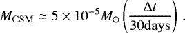 (5)
(5)
CSM energetics. Our CMFGEN models indicate a minimum radiative luminosity of LRAD = 1.8 × 10⁶ L⊙ and kinetic luminosity of LKIN = 1.2186 × 10⁴ L⊙. Assuming a duration of the stellar wind ejection of 30 days, this corresponds to a radiated energy of ERAD ≃ 1.8 × 1046 erg and kinetic energy of EKIN = 1.26 × 1044 erg. This leads to a radiative efficiency of ϵ = ERAD∕EKIN ≃140, which is within the range expected for stellar winds of hot massive stars.
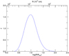 |
Fig. 4 Formation region of the Hα line as a function of distance to the star. The quantity ξ is related to the equivalent width of the line as |

3.3 Sensitivity of the derived parameters and model degeneracies
In this section, we explore possible degeneracies of our best-fit model by analysing a grid of synthetic CMFGEN spectra covering a large parameter space.
Temperature. Figure 5a shows a set of models with L⋆ = 2.7 × 10⁶ L⊙, Ṁ = 10−3 M⊙ yr−1, v∞ = 1000km s−1, identical abundances (Table 2), and different T⋆ in the range 10200−20700 K. Going from lower to higher temperatures, the emission of all H I lines (see Hα in Fig. 5c) and Fe II lines (Fig. 5) increases. This happens because an increase in T⋆ leads to more H ionisation, up to the point where H is essentially fully ionised in the region of the CSM where Hα originates. The only line not affected by the effective temperature is Na I λ5889 Å because Na is completely neutral in this temperature range.
Mass-loss rate. Another factor that shapes the ionisation structure is the mass-loss rate. Figure 5d contains a set of models with fixed L⋆, v∞, and abundances (Table 2), but exploring variations in Ṁ from 10−4 to 10−2 M⊙ yr−1. A model with Ṁ = 10−4 M⊙ yr−1 (red line in Fig. 5d) underestimates all emission lines compared to the observed spectrum. Increasing Ṁ by a factor of 2 (orange line in Fig. 5d) produces a better fit of the Hα line (Fig. 5f), but grossly underestimates Fe II λλ5198, 5235, 5276, 5317 Å (Fig. 5e). At Ṁ ≥ 4.5 × 10⁻⁴ M⊙ yr−1, the H I emission lines decreases. For example, a model with Ṁ = 6.7 × 10⁻⁴ M⊙ yr−1 shows a lower H I emission than observed. A model with Ṁ somewhere in the range 4.5 × 10⁻⁴ – 6.7 × 10⁻⁴ M⊙ yr−1 would also fit the observed spectrum. Raising Ṁ to values higher than 6.7 × 10⁻⁴ M⊙ yr−1 results in less H I emission. This is caused by the recombination of ionised hydrogen into neutral hydrogen. Figure 6 shows that as Ṁ increases, more and more ionised hydrogen recombines. When we reach Ṁ = 6.7 × 10⁻⁴ M⊙ yr−1, neutral hydrogen dominates in the formation region of Hα, leading to reduced emission. In these models the temperature varies slightly together with the mass-loss rates, due to the method we followed in developing this grid. As previously explained, an increase in temperature would lead to an increased strength of the emission lines; therefore, the increasing temperature in the lower mass-loss rate side only leads to a faster increase in ionisation. In other words, if we had a model with T⋆ = 10 000 K, we would need a much lower mass-loss rate to find a fit for the H β emission. Models with Ṁ < 3 × 10⁻⁴ M⊙ yr−1 do not fit the observed spectrum, since no satisfactory fit can be simultaneously obtained for Hα, Hβ, and Fe II lines in this regime. For Ṁ < 3 × 10⁻⁴ M⊙ yr−1, the Fe II lines are too weak and an increase in temperature is needed to fit H β and Hβ. However, this causes He I λ5875.66 Å emission on the red side of Na I λ5889.95 Å in the synthetic spectrum, which does not fit the observations.
On the high Ṁ end, changes in Ṁ have a much greater impact on the models. For example, for Ṁ = 1.5 × 10⁻³ M⊙ yr−1 we already require T⋆ ≃ 19 500 K to find a reasonable fit for the observations. For Ṁ > 2.3 × 10⁻³ M⊙ yr−1 we were not able not fit the emission lines since all H is already ionised. Therefore, a further increase in temperature would not lead to Hα emission comparable to the observations.
Clumping. Our models underestimate the observed red-wing emission of the H β and Hβ lines (Fig. 2). Models with unclumped winds show increased electron scattering emission as expected (Hillier 1991); however, this is not sufficient to explain the feature observed in our spectrum (Fig. 7). The origin of this feature is not clear. One possibility is that the progenitor at this point has a time-dependent wind. Another possibility would be that the velocity structure is more complex than our assumptionsand presents regions of higher wind velocities. If the outflow is indeed unclumped, then a higher Ṁ than that quoted in Table 2 is required to fit the observed spectrum. For example, the unclumped wind model shown in Fig. 7 has Ṁ = 6 × 10⁻³ M⊙ yr−1. This is not proportionalto  due to the change in the optical depth structure.
Velocity law. As mentioned in Sect. 2, the β parameter gives the steepness of the velocity law, thus changing the density structure in the inner regions. A decrease in β would require an increase in Ṁ in order to keep ρ constant. Our models show that a decrease to a value of β = 1, overestimates the emission lines. The spectrum fits well again once Ṁ is increased to 1.65× 10⁻³M⊙ yr−1. Given the relatively small change in Ṁ due to the change in the β parameter, the variation in β is covered in the range we determined for Ṁ. In addition, the shape of the emission line is slightly affected by the change in the velocity/density structure, and our β =1 model clearly shows a poorer fit to the line morphology.
Abundances. Figure 5g shows the spectra of three models that are identical in every way except for the abundances of H and He: the red spectrum is our best-fit model discussed in Sect. 3.1, having the abundances presented in Table 2 (i.e. X = 0.5); the orange spectrum is a model having X = 0.25; and the brown spectrum is a model with X = 0.75. We expected that an increase in the H abundance would lead to stronger emission, but we observed the opposite effect where the X = 0.25 spectrum has a stronger H β emission line than any of the higher abundance models. The explanation is similar to the increased Ṁ case. In this T⋆ range, having more H in the CSM leads to more recombination to neutral hydrogen, and therefore a decrease in the strength of the H emission lines.
The Fe II λλ4924, 5018, 5169 Å lines also show increased strength for a lower H content even if the Fe abundance remains unchanged. Changes in the H or the Fe abundances will have an effect on both ionisation structures, ultimately affecting the H and Fe line strengths. In addition, a change in the H abundance also affects the temperature structure, due to the different opacity of H and He. Taking into account the effect of the temperature on the H emission, a decrease in T⋆ to only 14000 K would lead to a well-fitted spectrum for the model with X = 0.25. Similarly, a small increase in T⋆ would lead to a good reproduction of the observed spectrum for a model with X = 0.75. This means that we have a poor constraint on the abundances based solely on this observed spectrum.
We also computed a model with X = 0.05 to investigate whether extremely low values of the H abundance would fit the observed spectrum. We found a poor fit that underestimates the H β and Hβ emission and overestimates all Fe II emission lines. Increasing the mass-loss rate to Ṁ = 3.4 × 10⁻³ M⊙ yr−1 and decreasing the Fe abundance to one-quarter of the solar Fe metallicity, we found a fit for most emission lines in the optical spectrum. However, the absorption component of the Na I λ5889 Å is now filled by the He Iλ5876 Å emission line, which is not observed. This is a good indication that we have overestimated the He abundance and, consequently, underestimated the amount of H.
To conclude, we find a number of combinations of model parameters that fit the observed spectrum. The mass-loss rate–temperature values are degenerate, but not enough to significantly affect the conclusions on the properties of the SN2015bh progenitor. We can confidently place our mass-loss rate in the 6 × 10⁻⁴–1.5 × 10⁻³ M⊙ yr−1 interval and the temperature between 13 000 and 19 500 K. The abundances of H and He are extremely difficult to determine by modelling the 12 November 2013 spectrum alone. We suggest that the H and He abundances could be better constrained by modelling the post-explosion spectra which simultaneously show the presence of H, He I, and He II lines.
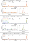 |
Fig. 5 Grid of CMFGEN synthetic spectra around the best-fit model of the 2015bh progenitor, exploring variations in T⋆ (panels a− c), Ṁ (panels d−f), and H abundance (panel g). The model parameters are indicated above each group of panels. |
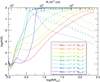 |
Fig. 6 H ionisation structure for SN2015bh progenitor models with different values of Ṁ. The continuous line represents the amount of neutral hydrogen, while the dotted line represents the ionised hydrogen. |
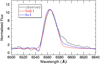 |
Fig. 7 Comparison of H β line between our best-fit model from Fig. 2 which has a clumped wind with f = 0.1 (red) and a model with an unclumped wind, i.e. f = 1 (blue). The observed spectrum is shown in grey. |
4 Discussion
4.1 Constraints on the exploding star: a warm LBV
Our CMFGEN models of the 12 November 2013 spectrum of SN 2015bh suggests that the progenitor had L⋆ = 1.8 − 4.7 × 10⁶ L⊙, T⋆ = 13 000−19 500 K, Teff= 8700−10 000K, Ṁ = 0.67−1.5 × 10⁻³ M⊙ yr−1, v∞ = 1000 km s−1, X = 0.25−0.75, and half-solar Fe abundance. We interpret the spectrum as arising from the extended photosphere and stellar wind, similar to other observed LBVs in the Galaxy and SMC. We do not see any obvious evidence for interaction in 12 November 2013. Let us now compare the SN2015bh progenitor properties with those of different classes of evolved massive stars.
The spectral morphology of the progenitor of SN2015bh strongly resembles an LBV. The luminosity computed in our model of a few times 106 L⊙ corresponds to typical LBV luminosities (~105−106.7 L⊙; van Genderen 2001; Smith et al. 2004; Clark et al. 2005, 2009; Groh et al. 2013). The temperature range of our model lies in the mid-range of LBV temperatures (8000−25 000 K; van Genderen 2001). LBVs have a wide range of possible mass-loss rates stemming from quiescent stellar winds or eruptions, from 10−5 to 1 M⊙ yr−1 (Smith 2014). Our determined value of Ṁ fits well within this range. Our models indicate v∞ = 1000 km s−1, which is higher than the velocities estimated for LBVs in the Milky Way and Magellanic Clouds (Smith et al. 2004). One of the highest observed velocities of an LBV outflow was during the Eta Carinae Great Eruption (v∞ = 600−800 km s−1; Smith 2006). Interestingly, Izotov & Thuan (2009) detected LBVs with fast winds (800 km s−1) in low-metallicity dwarf galaxies; this value is more in line with our derived v∞ for the SN2015bh progenitor. Our derived value of Ṁ is on the high side for LBVs in quiescence, being similar to that of the current wind of Eta Car (Hillier et al. 2001; Groh et al. 2012). While radiation pressure on lines and continuum could drive the winds of Eta Car (Hillier et al. 2001) and other bona fide LBVs such as AG Car (Groh et al. 2009b, 2011), we cannot exclude that the star possesses a dynamic super-Eddington wind (Shaviv 2001; Owocki et al. 2004; van Marle et al. 2009), especially in epochs when MR ≲−12 mag. We note that if the progenitor of SN 2015bh is in a super-Eddington state, our previously derived Mmin is not applicable.
Our results reinforce the suggestions from previous studies that the progenitor of SN2015bh is an LBV. Thöne et al. (2017) propose that the pre-explosion spectrum is very similar to that of a quiescent LBV, based on the combined stellar evolution and atmospheric models from Groh et al. (2014). Goranskij et al. (2016) support the LBV progenitor scenario based on the argument that the brightness measurements from 6 March 2008 are close to the Humphreys & Davidson limit. Elias-Rosa et al. (2016) also conclude that the progenitor of SN2015bh was likely a massive blue star.
The high v∞ could instead be indicative of a Wolf–Rayet (WR) progenitor. However, the derived value of Teff for the SN2015bh progenitor is significantly below typical values for the Teff of WRs (30 000−150 000 K; Crowther 2007; Sander et al. 2012). A more plausible possibility is that the progenitor of SN2015bh was a WR star that inflated just before eruption, that it was a star with an increased envelope radius due to the star’s proximity to the Eddington limit. This would in principle decrease the effective temperature. Gräfener et al. (2012) showed through numerical models that the effective temperature of a H-poor WR (X < 0.05) can be reduced from 100 000 to 40 000 K through envelope inflation, while LBVs of solar abundances can have Teff as low as 16 000 K when inflation takes place. While none of the models presented in Gräfener et al. (2012) matches our SN2015bh properties, we cannot exclude the possibility of an inflated WR progenitor, especially since our CMFGEN model is very close to the Eddington limit in the deep atmospheric layers (Γ ~ 0.85−0.90).
We can exclude a red supergiant (RSG) or yellow hypergiant (YHG) progenitor for SN2015bh, since RSGs have temperatures of at most 6000 K (Levesque et al. 2005; Davies et al. 2013) and YHGs are in the range 4000–8000 K (Kovtyukh 2007) and the wind velocities of these types of stars typically reach 100 km s−1 (de Jager 1998). Thöne et al. (2017) discusses the possibility of a YHG progenitor based on the photometry and on the assumption that prior to 2013 the star was quiescent. While the authors raise it as a viable option, they question thelack of dust surrounding the progenitor, which would be expected in stars at low temperature and high v∞.
Even if the values of Teff, L⋆, and v∞ are consistent with those of supergiant B[e] stars (sgB[e]), which typically have Teff ~ 10 000−25 000 K and L⋆ > 104 L⊙ (Lamers et al. 1998), the absence of forbidden lines is a clear indication that the progenitor of SN2015bh was not a B[e] star. Furthermore, sgB[e] stars generally do not exhibit the large photometric variations seen in the progenitor of SN2015bh, and the lack of an infrared excess is also at odds with a B[e] classification.
4.2 Is the progenitor of SN2015bh an interacting binary
Since a significant fraction of massive stars are found in binary systems (Sana et al. 2012; Sana 2017), we now explore the possibility that the SN2015bh progenitor had a companion star. This scenario is attractive especially because the LBV-like properties of the progenitor of SN 2015bh (Sect. 3.1) before the 2015 events bare significant resemblance to those of HD 5980, in particular the L⋆, T⋆, Ṁ, and v∞. In addition, the similarity in the light curve variation pattern and timescale raises the question of whether the SN 2015bh progenitor’s system was similar to HD 5980 but later underwent a powerful, and perhaps terminal, explosion.
HD 5980 is a massive multiple star system in the Small Magellanic Cloud (Koenigsberger et al. 2006). It is formed of an eclipsing pair of stars, stars A and B, and star C, which is itself a binary (Nazé et al. 2018). The system showed long-term variability in the light curve for ~40 yr and sudden variability in 1993 and 1994. The cause of the long-term variation is believed to be due to one of the stars in the system, star A, an LBV undergoing S Doradus variability. The properties of star A have undergone rapid changes, especially during the 1994 event, having v∞ = 500−2440 km s−1, unclumped Ṁ = 10−5−10−4 M⊙ yr−1, Teff = 23 000−43 000 K, log (L∕L⊙) = 6.3−7.05 (Georgiev et al. 2011).
Gräfener et al. (2012) suggest that star A in HD5980 could have been an inflated LBV during its 1994 event due to the proximity to the Eddington limit. The increase in radius could trigger an eruption, in a similar fashion to that proposed by Smith (2011) to explain the 1840 Eta Carinae eruption. For 2015bh, the sudden increases in absolute magnitude in the 2008 and 2013 events could also be triggered by envelope inflation followed by binary interaction, especially because our models indicate that the star is likely close to the Eddington limit.
A binary scenario has also been advocated in the context of the pre-explosion outbursts of SN 2009ip (Mauerhan et al. 2013) and SN 2015bh (Soker & Kashi 2016). If the SN 2015bh progenitor is in a binary system, the secondary star would have to be much fainter than the primary since we do not see any evidence of spectral lines from the companion in the optical spectrum from 12 November 2013. A higher cadence over a long period of time would be required to obtain orbital information of the putative binary system. Future high-cadence surveys such as the Large Synoptic Survey Telescope (LSST) could possibly observe the progenitors of events similar to that of SN2015bh and establish their long-term photometric behaviour with unprecedented detail.
4.3 Implications and comparison to other LBVs and interacting supernovae
While it was originally thought that LBVs could not be direct progenitors of SNe and would instead always evolve to WR stars, recent observationsand modelling have strongly suggested otherwise. Figure 8 shows the location of the SN2015bh progenitor in the HR diagram, together with those of galactic LBVs and interacting SNe with similar light curves for which determinations of L and Teff exist in the literature. The temperature range of the SN2015bh progenitor compares well to other LBVs, while the luminosity places our progenitor at the high end of LBV luminosities. While the temperature of the SN2009ip progenitor is poorly constrained, our results indicate that the progenitor of SN2015bh is slightly more luminous than that of SN2009ip even though the two light curves are extremely similar. The placement in the HR diagram of the progenitor of SN 2015bh also points to an initial mass of M ≃ 150−200 M⊙.
Significantly, more information exists about the progenitor Ṁ and v∞ of SNe with light curves similar to SN 2015bh. Figure 9 compares the Ṁ and v∞ derived for both terminal and non-terminal events. We can see that while they all have similar values of Ṁ and v∞ characteristic of LBVs, the range of values likely indicates that these events do not have exactly the same progenitor, but rather span a range of masses and luminosities.
SN2005gl is believed to have a M⋆ > 50 M⊙ LBV progenitor (Gal-Yam et al. 2007) that ejected an outflow with Ṁ = 0.03 M⊙ yr−1 and v∞≃ 420 km s−1 (Gal-Yam & Leonard 2009);
SN2010jl likely originated from a >30 M⊙ star (Smith et al. 2011) that had a high Ṁ of 0.1 M⊙ yr−1 before exploding (Fransson et al. 2014; Dessart et al. 2015);
SN2009ip shows almost identical photometry to SN2015bh and signs of LBV-like behaviour (Thöne et al. 2017); the mass-loss rate of the SN2009ip progenitor was determined by Ofek et al. (2013) to be 10−3–10−2 M⊙ yr−1 and v∞≃ 1000 km s−1, while Moriya (2015) suggested an LBV progenitor with Ṁ = 0.1 M⊙ yr−1 and v∞ = 550 km s−1;
SN2002kg has a lower velocity of v∞ = 320 km s−1 (Van Dyk et al. 2006) and Ṁ is unconstrained;
SN2000ch displays the highest wind velocity in this sample (800 km s−1; Wagner et al. 2004), which is similar to what we found for the SN2015bh progenitor;
SNhunt248 is another event exhibiting a very similar behaviour to SN2015bh in light curve, spectra and the lack of dust in its close environment; however, the SNhunt248 spectrum suggests a lower wind velocity of <300 km s−1 (Kankare et al. 2015).
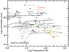 |
Fig. 8 HR diagram showing the location of the progenitor of SN2015bh as determined in this work (red). We include the progenitor of SN2009ip (blue; Smith et al. 2010; Foley et al. 2011), SN2010jl (green; Smith et al. 2011), UGC2773-OT (yellow; Smith et al. 2010), and Gaia16cfr (orange; Kilpatrick et al. 2018). For reference, we show the location of Galactic LBVs in quiescence (black squares; Groh et al. 2013 and references therein) and Geneva evolutionary tracks for single stars at solar metallicity (Ekström et al. 2012; Georgy et al. 2012; Groh et al. 2013). |
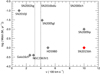 |
Fig. 9 Comparison between the wind/CSM velocities and mass-loss rates of interacting SNe similar to SN2015bh. The values for SN2015bh (red) are taken from this work, and the references for the other events are as follows: SN2005gl – Gal-Yam& Leonard (2009); SN2010jl – Fransson et al. (2014); Dessart et al. (2015); SN2009ip – Ofek et al. (2013); SN2002kg – Van Dyk et al. (2006); SN2000ch – Wagner et al. (2004); HD5890 – Georgiev et al. (2011); NGC2363v1 – Drissen et al. (2001); Gaia16cfr – Kilpatrick et al. (2018); and SN2016bdu – Pastorello et al. (2018). |
4.4 Constraints on the post-explosion behaviour
Having previously discussed the properties of the SN2015bh progenitor, let us examine the possible scenarios for the post-explosion behaviour of SN2015bh in light of our new findings. We follow the definition of t = 0 as 24 May 2015, i.e. at the peak of the 2015B event, as in Thöne et al. (2017). Thus, the 12 November 2013 spectrum was taken at t = −558.8 d and the peak of the 2015A event was at t ≃−25 d.
We begin this subsection by briefly summarising the scenarios that have been proposed in the literature.
Interaction of two shells + dense CSM (Thöne et al. 2017). In this scenario, a first thin shell with v = 700 km s−1 would be ejected years prior to 2015 B, giving rise to the absorption component observed at t = −558.8 d (see their Fig. 13). Then, a second shell with ≃ 2200−2300 km s−1 would be ejected at the time of the 2015 A event, which could be the ejecta of a genuine SN or SN impostor. The second shell would appear first in absorption and, about 100 days later, catch up with the first shell and produce the 2000 km s−1 emission component by shock excitation. These authors also proposed that at late times the 2300 km s−1 shell interacts with a dense CSM that had been previously created by the progenitor. The Thöneet al. (2017) model reproduces the late evolution of the light curve with a shell of mass Ms =~ 0.005−0.5 M⊙ and vs = 2300 km s−1 interacting with a CSM created by a progenitor mass-loss rate of Ṁ ≃ 0.005 M⊙ yr−1. This is 3–10 times higher than the Ṁ we determined from our CMFGEN models. Radiative hydrodynamic models can be used to infer the explosion energy, mass, energy released in the wind, and the expansion velocity of the shocked shell given our determined wind properties and the light curve evolution. See Moriya (2015) for a more detailed comparison to the existing literature.
SN ejecta + fallback + CSM interaction with multiple shells (Elias-Rosa et al. 2016). These authors propose that a ~ 1000km s−1 shell was expelled around 2002 or before to explain the pre-explosion spectrum. They conclude that an outburst at the end of 2013 with material moving at 1000 km s−1 produced the increase in luminosity observed in December 2013. They propose that the 2015 A event was a core-collapse SN that experienced large fallback of material, thus explaining the low energy. They also infer the presence of three emission components in H β, which would be an argument for core-collapse, as a multi-component H β is typical of interacting SNe. Then at t = 0, the newly ejected material collides with a slow, dense CSM and produces 2015 B. After the shock passes, the two absorption components (1000 km s−1 and 2100 km s−1) are visible again. They attribute this to at least two shells or clumps of cooler material moving in the observer’s direction.
Our findings imply that the pre-explosion spectrum from t = −558.8 d is formed in an extended CSM, unlike Thöne et al. (2017) and Elias-Rosa et al. (2016) who have proposed that the pre-explosion spectrum was formed in a thin shell. We propose that the subsequent interaction occurs mainly with the extended material, eliminating the necessity of the first shell ejection proposed in Thöne et al. (2017). Figure 10a shows our proposed geometry at t = −558.8 d based on our derived values of R⋆ = 5.1−25.9 × 1012 cm, T⋆ = 13 000−19 000 K, L⋆ = 1.8−4.7 × 10⁶ L⊙, Ṁ = 0.6−1.5 × 10⁻³ M⊙ yr−1, and v∞ = 1000 km s−1. Given that the progenitor star had similarly high luminosities for at least 20 yr before the eruption, during this period the star most likely had a wind at least as dense as that we have inferred for t = −558.8 d. This long-term wind produces an extended CSM with RCSM ≳ 2.57 × 1014 cm (see Sect. 3.2). The wind needs to be ejected at least 30 days prior to the 12 November 2013 observations, i.e. t = −589 d, in order to produce the observed emission. While our stationary models yield an outflow with ρ ∝ r−2 at large distances, the extended pre-explosion CSM around SN 2015bh is most likely inhomogeneous given the significant variability before explosion (Elias-Rosa et al. 2016; Ofek et al. 2016; Thöne et al. 2017).
We support the suggestion from Thöne et al. (2017) that an explosion (although not necessarily terminal) occurs around t ≃ −40 days, when a second absorption component at −2000 km s−1 is observed in the H β line profile. However, we propose that the double absorption line profile is generated by a 2000 km s−1 shell expanding into an extended CSM produced by a long-term 1000 km s−1 wind. Figure 10b sketches how the CSM would look at this stage according to our scenario (cf. Fig. 13 in Thöne et al. 2017).
At this point, it is uncertain whether the star has survived. At about t = +26 d, the spectrum of SN 2015bh clearly shows two absorption components at ~ −1000 km s−1 and −2000 km s−1, and by t = 100 d H β has the two components in emission (Elias-Rosa et al. 2016; Thöne et al. 2017). These authors have also reported that at t = +242 days, the two-peak emission is still present; in our scenario the fast shell would be at 5 × 1015 cm at this time. As the shell expands, it eventually becomes optically thin at very late times (t ≫ 250 days). Below, we analyse two scenarios for t ≫ 250 days depending on whether the star survived or collapsed.
Scenario 1 (surviving star). We explore the scenario in which the star is still present after the main event, as originally proposed by Thöneet al. (2017). At first the star should be out of thermal equilibrium, and should then re-establish a stellar wind. For t ≫ 250 days, we should see both emission from the optically thin shell and from the new wind/CSM of the star inside the shell (Fig. 10c). In this case late time spectroscopy should reveal the presence of the new wind and CSM. The star could slowly relax back to its original LBV state or become a Wolf–Rayet star, depending how the mass of the H envelope before the explosion compares to the mass ejected in the process (~ 0.5 M⊙; Thöne et al. 2017). Curiously, the spectrum of SN2009ip at + 581 days (Thöne et al. 2017) bares a significant resemblance to the SN2015bh spectrum from 12 November 2013, showing prominent H β and Hβ lines, multiple Fe II lines, and the Na I λ5889Å with a strong absorption component. Our scenario of a surviving star is similar to that proposed by Thöne et al. (2017), with the exception that we consider only one high-velocity, optically thin shell expanding into an extended CSM created by the progenitor.
Scenario 2. If the star did not survive, the 1000 km s−1 component would have to come from outside of the 2000 km s−1 shell. Since we propose that the 1000 km s−1 component arises in the extended progenitor wind, this component should become weak and eventually disappear for t ≫ 250 days. There is the possibility that the shell is still interacting with the former CSM (Fig. 10d), which would further support our argument that the progenitor had an extended wind and not a thin shell prior to 2015A. If the star exploded as a genuine SN, 2015bh would be a remarkable case of a successful core collapse of a star of at least 35 M⊙ at the pre-SN stage.
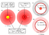 |
Fig. 10 Sketch of the CSM geometry around SN2015bh at selected epochs. Panel a: pre-explosion extended CSM derived in this paper; panel b: expansion of the ejected shell into the extended CSM assuming the shell is ejected at t ≃ −40 days, hence the radius of the shell Rshell = R⋆ at this stage; panel c: post-explosion scenario where the star survived; and panel d: post-explosion scenario for a supernova explosion. |
5 Summary and conclusions
In this paper, we investigated the progenitor of SN2015bh by means of CMFGEN radiative transfer modelling of the spectrum obtained 559 days prior to the main event. Here we summarise our main findings:
- 1.
We perform radiative transfer modelling of the SN2015bh progenitor using CMFGEN. Our models assume extended, clumped, steady, spherically symmetric wind in non-local thermodynamic equilibrium following a β-type velocity law and having the density structure ρ ∝ r−2.
- 2.
By running an extensive grid of models we conclude that the models are degenerate and a good fit could be reproduced by stars with slightly different physical properties. While T⋆ and Ṁ are constrained in relatively small intervals of 13 000 to 19 500 K corresponding to Ṁ = 6 × 10⁻⁴–1.5 × 10⁻³ M⊙ yr−1, the H abundance shows a wide range of values. We can fit the spectrum reasonably well for a model with X = 0.25, T⋆ = 14 000 K, Ṁ = 10−3 M⊙ yr−1 and for another model with X = 0.75, T⋆ ≃ 15 300 K, Ṁ = 10−3 M⊙ yr−1.
- 3.
For L⋆ = 1.8 × 10⁶ L⊙, R⋆ = 5.15 × 1012 cm, T⋆ = 19 500 K, Ṁ = 0.6 × 10⁻³ M⊙ yr−1, and v∞ = 1000 km s−1 the emission observed in the spectrum is generated in the CSM up to RCSM = 2.57 × 1014 cm. The wind needs to have started at least 30 days prior to the 12 November 2013 observations in order to fill out RCSM at the determined Ṁ and v∞. The mass of material contained in this region is MCSM = 0.5 × 10⁻⁴ M⊙.
- 4.
Based on the values of our best-fit models, we propose that the progenitor of SN2015bh is either a warm LBV or an inflated WR star of at least 35 M⊙. This type of progenitor matches other types of SNIIn/impostors progenitors.
- 5.
We conclude that the progenitor of SN2015bh had a strong extended wind which interacted with a faster shell moving at 2000 km s−1. We were not able to determine whether the star exploded as a SN or not, but we do propose two scenarios. In the case of a non-terminal eruption, the star could reinstate its previous wind or become a WR, and at very late times (t ≫ 250 days) we should see emission from the 2000 km s−1 shell, which has become optically thin, and the stellar wind/CSM. In the case of a SN, the shell could be interacting with the extended CSM, even at t ≫ 250 days, and possibly produce observable signatures. The level of late-time interaction will depend on both the CSM and the SN ejecta properties and a detailed hydrodynamics model of the entire light curve would be needed to fully investigate this aspect. Similar conclusions have been reached by Thöne et al. (2017) and Elias-Rosa et al. (2016) with themain difference being that the previous works propose that the possible SN ejecta interacts with multiple thin shells, while our work strongly supports interaction with an extended CSM. The different scenarios investigated above can be tested via future observations of SN 2015bh at late times.
SN2015bh is comparable to many other events, such as SN2009ip, SNhunt248, and HD5980. Due to the unique pre-explosion spectrometry, we were able to constrain the properties of the SN2015bh progenitor and, by extension, add to the still incomplete picture of SN progenitors and SN impostors. Our results contribute to our understanding of the members of this new growing class of events and the pre-supernova evolution of massive stars.
Acknowledgements
I.B. acknowledges funding from a Trinity College Postgraduate Award through the School of Physics, and J.H.G. acknowledges support from an Irish Research Council New Foundations Award 206086.14414 “Physics of Supernovae and Stars”. The authors are grateful to Ylva Götberg for making available her python scripts for CMFGEN, and thank C. Thöne, T. Moriya, and J.S. Vink for discussions on interacting supernovae and SN2015bh. We would like to thank the other researchers in the Astrophysics group at Trinity College Dublin for helpful discussions.
References
- Anderson, L. S. 1989, ApJ, 339, 558 [NASA ADS] [CrossRef] [Google Scholar]
- Busche, J. R., & Hillier, D. J. 2005, AJ, 129, 454 [NASA ADS] [CrossRef] [Google Scholar]
- Chevalier, R. A., & Fransson, C. 1994, ApJ, 420, 268 [NASA ADS] [CrossRef] [Google Scholar]
- Chugai, N. N. 2001, MNRAS, 326, 1448 [NASA ADS] [CrossRef] [Google Scholar]
- Chugai, N. N., Blinnikov, S. I., Cumming, R. J., et al. 2004, MNRAS, 352, 1213 [NASA ADS] [CrossRef] [Google Scholar]
- Clark, J. S., Larionov, V. M., & Arkharov, A. 2005, A&A, 435, 239 [NASA ADS] [CrossRef] [EDP Sciences] [Google Scholar]
- Clark, J. S., Crowther, P. A., Larionov, V. M., et al. 2009, A&A, 507, 1555 [NASA ADS] [CrossRef] [EDP Sciences] [Google Scholar]
- Crowther, P. A. 2007, ARA&A, 45, 177 [NASA ADS] [CrossRef] [Google Scholar]
- Davies, B., Kudritzki, R.-P., Plez, B., et al. 2013, ApJ, 767, 3 [NASA ADS] [CrossRef] [Google Scholar]
- de Jager C. 1998, A&ARv., 8, 145 [NASA ADS] [CrossRef] [Google Scholar]
- de Jager, C., Nieuwenhuijzen, H., & van der Hucht, K. A. 1988, A&AS, 72, 259 [NASA ADS] [Google Scholar]
- Dessart, L., Hillier, D. J., Gezari, S., Basa, S., & Matheson, T. 2009, MNRAS, 394, 21 [NASA ADS] [CrossRef] [Google Scholar]
- Dessart, L., Audit, E., & Hillier, D. J. 2015, MNRAS, 449, 4304 [NASA ADS] [CrossRef] [Google Scholar]
- Drissen, L., Crowther, P. A., Smith, L. J., et al. 2001, ApJ, 546, 484 [NASA ADS] [CrossRef] [Google Scholar]
- Ekström, S., Georgy, C., Eggenberger, P., et al. 2012, A&A, 537, A146 [NASA ADS] [CrossRef] [EDP Sciences] [Google Scholar]
- Elias-Rosa, N., Pastorello, A., Benetti, S., et al. 2016, MNRAS, 463, 3894 [NASA ADS] [CrossRef] [Google Scholar]
- Elias-Rosa, N., Benetti, S., Tomasella, L., et al. 2015, ATel, 7042 [Google Scholar]
- Fassia, A., Meikle, W. P. S., Chugai, N., et al. 2001, MNRAS, 325, 907 [NASA ADS] [CrossRef] [Google Scholar]
- Fitzpatrick, E. L. 1999, PASP, 111, 63 [NASA ADS] [CrossRef] [Google Scholar]
- Foley, R. J., Berger, E., Fox, O., et al. 2011, ApJ, 732, 32 [NASA ADS] [CrossRef] [Google Scholar]
- Fransson, C., Ergon, M., Challis, P. J., et al. 2014, ApJ, 797, 118 [NASA ADS] [CrossRef] [Google Scholar]
- Fraser, M., Kotak, R., Pastorello, A., et al. 2013, ATel, 4953, 1 [NASA ADS] [Google Scholar]
- Fraser, M., Kotak, R., Pastorello, A., et al. 2015, MNRAS, 453, 3886 [NASA ADS] [CrossRef] [Google Scholar]
- Gal-Yam, A., & Leonard, D. C. 2009, Nature, 458, 865 [NASA ADS] [CrossRef] [PubMed] [Google Scholar]
- Gal-Yam, A., Leonard, D. C., Fox, D. B., et al. 2007, ApJ, 656, 372 [NASA ADS] [CrossRef] [Google Scholar]
- Gal-Yam, A., Arcavi, I., Ofek, E. O., et al. 2014, Nature, 509, 471 [NASA ADS] [CrossRef] [Google Scholar]
- Georgiev, L., Koenigsberger, G., Hillier, D. J., et al. 2011, AJ, 142, 191 [NASA ADS] [CrossRef] [Google Scholar]
- Georgy, C., Ekström, S., Meynet, G., et al. 2012, A&A, 542, A29 [NASA ADS] [CrossRef] [EDP Sciences] [Google Scholar]
- Goranskij, V. P., Barsukova, E. A., Valeev, A. F., et al. 2016, ArXiv e-prints [arXiv:1609.00731] [Google Scholar]
- Gräfener, G., & Vink, J. S. 2016, MNRAS, 455, 112 [NASA ADS] [CrossRef] [Google Scholar]
- Gräfener, G., Owocki, S. P., & Vink, J. S. 2012, A&A, 538, A40 [NASA ADS] [CrossRef] [EDP Sciences] [Google Scholar]
- Graham, M. L., Bigley, A., Mauerhan, J. C., et al. 2017, MNRAS, 469, 1559 [NASA ADS] [CrossRef] [Google Scholar]
- Groh, J. H. 2014, A&A, 572, L11 [NASA ADS] [CrossRef] [EDP Sciences] [Google Scholar]
- Groh, J. H., Damineli, A., Hillier, D. J., et al. 2009a, ApJ, 705, L25 [NASA ADS] [CrossRef] [Google Scholar]
- Groh, J. H., Hillier, D. J., Damineli, A., et al. 2009b, ApJ, 698, 1698 [NASA ADS] [CrossRef] [Google Scholar]
- Groh, J. H., Hillier, D. J., & Damineli, A. 2011, ApJ, 736, 46 [NASA ADS] [CrossRef] [Google Scholar]
- Groh, J. H., Hillier, D. J., Madura, T. I., & Weigelt, G. 2012, MNRAS, 423, 1623 [NASA ADS] [CrossRef] [Google Scholar]
- Groh, J. H., Meynet, G., Georgy, C., & Ekström, S. 2013, A&A, 558, A131 [NASA ADS] [CrossRef] [EDP Sciences] [Google Scholar]
- Groh, J. H., Meynet, G., Ekström, S., & Georgy, C. 2014, A&A, 564, A30 [NASA ADS] [CrossRef] [EDP Sciences] [Google Scholar]
- Hillier, D. J. 1991, A&A, 247, 455 [NASA ADS] [Google Scholar]
- Hillier, D. J., & Miller, D. L. 1998, ApJ, 496, 407 [NASA ADS] [CrossRef] [Google Scholar]
- Hillier, D. J., Crowther, P. A., Najarro, F., & Fullerton, A. W. 1998, A&A, 340, 483 [NASA ADS] [Google Scholar]
- Hillier, D. J., Davidson, K., Ishibashi, K., & Gull, T. 2001, ApJ, 553, 837 [NASA ADS] [CrossRef] [Google Scholar]
- Izotov, Y. I., & Thuan, T. X. 2009, ApJ, 690, 1797 [NASA ADS] [CrossRef] [Google Scholar]
- Kankare, E., Kotak, R., Pastorello, A., et al. 2015, A&A, 581, L4 [NASA ADS] [CrossRef] [EDP Sciences] [Google Scholar]
- Kiewe, M., Gal-Yam, A., Arcavi, I., et al. 2012, ApJ, 744, 10 [NASA ADS] [CrossRef] [Google Scholar]
- Kilpatrick, C. D., Foley, R. J., Drout, M. R., et al. 2018, MNRAS, 473, 4805 [NASA ADS] [CrossRef] [Google Scholar]
- Koenigsberger, G., Fullerton, A. W., Massa, D., & Auer, L. H. 2006, AJ, 132, 1527 [NASA ADS] [CrossRef] [Google Scholar]
- Kovtyukh, V. V. 2007, MNRAS, 378, 617 [NASA ADS] [CrossRef] [Google Scholar]
- Lamers, H. J. G. L. M., Zickgraf, F.-J., de Winter, D., Houziaux, L., & Zorec, J. 1998, A&A, 340, 117 [NASA ADS] [Google Scholar]
- Langer, N. 2012, ARA&A, 50, 107 [NASA ADS] [CrossRef] [Google Scholar]
- Leonard, D. C., Filippenko, A. V., Barth, A. J., & Matheson, T. 2000, ApJ, 536, 239 [NASA ADS] [CrossRef] [Google Scholar]
- Levesque, E. M., Massey, P., Olsen, K. A. G., et al. 2005, ApJ, 628, 973 [NASA ADS] [CrossRef] [Google Scholar]
- Levesque, E. M., Stringfellow, G. S., Ginsburg, A. G., Bally, J., & Keeney, B. A. 2014, AJ, 147, 23 [Google Scholar]
- Maeder, A., & Meynet, G. 2000, ARA&A, 38, 143 [NASA ADS] [CrossRef] [Google Scholar]
- Margutti, R., Milisavljevic, D., Soderberg, A. M., et al. 2014, ApJ, 780, 21 [NASA ADS] [CrossRef] [Google Scholar]
- Mauerhan, J., & Smith, N. 2012, MNRAS, 424, 2659 [NASA ADS] [CrossRef] [Google Scholar]
- Mauerhan, J. C., Smith, N., Filippenko, A. V., et al. 2013, MNRAS, 430, 1801 [NASA ADS] [CrossRef] [Google Scholar]
- Moriya, T. J. 2015, ApJ, 803, L26 [NASA ADS] [CrossRef] [Google Scholar]
- Najarro, F. 2001, in P Cygni 2000: 400 Years of Progress, eds. M. de Groot, & C. Sterken, ASP Conf. Ser., 233, 133 [NASA ADS] [Google Scholar]
- Najarro, F., Hillier, D. J., & Stahl, O. 1997, A&A, 326, 1117 [NASA ADS] [Google Scholar]
- Najarro, F., Figer, D. F., Hillier, D. J., Geballe, T. R., & Kudritzki, R. P. 2009, ApJ, 691, 1816 [NASA ADS] [CrossRef] [Google Scholar]
- Nazé, Y., Koenigsberger, G., Pittard, J. M., et al. 2018, ApJ, 853, 164 [NASA ADS] [CrossRef] [Google Scholar]
- Ofek, E. O., Lin, L., Kouveliotou, C., et al. 2013, ApJ, 768, 47 [NASA ADS] [CrossRef] [Google Scholar]
- Ofek, E. O., Cenko, S. B., Shaviv, N. J., et al. 2016, ApJ, 824, 6 [NASA ADS] [CrossRef] [Google Scholar]
- Owocki, S. P., Gayley, K. G., & Shaviv, N. J. 2004, ApJ, 616, 525 [NASA ADS] [CrossRef] [Google Scholar]
- Pastorello, A., Cappellaro, E., Inserra, C., et al. 2013, ApJ, 767, 1 [NASA ADS] [CrossRef] [Google Scholar]
- Pastorello, A., Kochanek, C. S., Fraser, M., et al. 2018, MNRAS, 474, 197 [NASA ADS] [CrossRef] [Google Scholar]
- Prieto, J. L., Brimacombe, J., Drake, A. J., & Howerton, S. 2013, ApJ, 763, L27 [NASA ADS] [CrossRef] [Google Scholar]
- Sana, H. 2017, IAU Symp., 329, 110 [Google Scholar]
- Sana, H., de Mink, S. E., de Koter, A., et al. 2012, Science, 337, 444 [Google Scholar]
- Sander, A., Hamann, W.-R., & Todt, H. 2012, A&A, 540, A144 [NASA ADS] [CrossRef] [EDP Sciences] [Google Scholar]
- Schlegel, E. M. 1990, MNRAS, 244, 269 [NASA ADS] [Google Scholar]
- Shaviv, N. J. 2001, ApJ, 549, 1093 [NASA ADS] [CrossRef] [Google Scholar]
- Shivvers, I., Groh, J. H., Mauerhan, J. C., et al. 2015, ApJ, 806, 213 [NASA ADS] [CrossRef] [Google Scholar]
- Smith, N. 2006, ApJ, 644, 1151 [NASA ADS] [CrossRef] [Google Scholar]
- Smith, N. 2011, MNRAS, 415, 2020 [NASA ADS] [CrossRef] [Google Scholar]
- Smith, N. 2014, ARA&A, 52, 487 [NASA ADS] [CrossRef] [MathSciNet] [Google Scholar]
- Smith, N., Vink, J. S., & de Koter A. 2004, ApJ, 615, 475 [NASA ADS] [CrossRef] [Google Scholar]
- Smith, N., Li, W., Foley, R. J., et al. 2007, ApJ, 666, 1116 [NASA ADS] [CrossRef] [Google Scholar]
- Smith, N., Miller, A., Li, W., et al. 2010, AJ, 139, 1451 [NASA ADS] [CrossRef] [Google Scholar]
- Smith, N., Li, W., Miller, A. A., et al. 2011, ApJ, 732, 63 [NASA ADS] [CrossRef] [Google Scholar]
- Smith, N., Mauerhan, J. C., & Prieto, J. L. 2014, MNRAS, 438, 1191 [NASA ADS] [CrossRef] [Google Scholar]
- Smith, N., Mauerhan, J. C., Cenko, S. B., et al. 2015, MNRAS, 449, 1876 [NASA ADS] [CrossRef] [Google Scholar]
- Soker, N., & Kashi, A. 2016, MNRAS, 462, 217 [NASA ADS] [CrossRef] [Google Scholar]
- Sollerman, J., Cumming, R. J., & Lundqvist, P. 1998, ApJ, 493, 933 [NASA ADS] [CrossRef] [Google Scholar]
- Stathakis, R. A., & Sadler, E. M. 1991, MNRAS, 250, 786 [NASA ADS] [Google Scholar]
- Thöne, C. C., de Ugarte Postigo, A., Leloudas, G., et al. 2017, A&A, 599, A129 [NASA ADS] [CrossRef] [EDP Sciences] [Google Scholar]
- Trundle, C., Kotak, R., Vink, J. S., & Meikle, W. P. S. 2008, A&A, 483, L47 [NASA ADS] [CrossRef] [EDP Sciences] [Google Scholar]
- Turatto, M., Cappellaro, E., Danziger, I. J., et al. 1993, MNRAS, 262, 128 [NASA ADS] [CrossRef] [Google Scholar]
- Van Dyk, S. D., Li, W., Filippenko, A. V., et al. 2006, ArXiv e-prints [arXiv:astro-ph/0603025] [Google Scholar]
- Van Dyk, S. D., Peng, C. Y., King, J. Y., et al. 2000, PASP, 112, 1532 [NASA ADS] [CrossRef] [Google Scholar]
- van Genderen A. M. 2001, A&A, 366, 508 [NASA ADS] [CrossRef] [EDP Sciences] [Google Scholar]
- van Marle, A. J., Owocki, S. P., & Shaviv, N. J. 2009, MNRAS, 394, 595 [NASA ADS] [CrossRef] [Google Scholar]
- Wagner, R. M., Vrba, F. J., Henden, A. A., et al. 2004, PASP, 116, 326 [NASA ADS] [CrossRef] [Google Scholar]
- Yaron, O., & Gal-Yam, A. 2012, PASP, 124, 668 [NASA ADS] [CrossRef] [Google Scholar]
- Yaron, O., Perley, D. A., Gal-Yam, A., et al. 2017, Nat. Phys., 13, 510 [NASA ADS] [CrossRef] [Google Scholar]
The inclusion of super levels is a technique used to decrease the number of levels whose atomic populations must be explicitly solved for (Anderson 1989; Hillier & Miller 1998), thus simplifying the calculations and improving computational time and memory requirements.
All Tables
CMFGEN model parameter ranges for the best-fitting models of the SN2015bh progenitor.
All Figures
|
Fig. 1 Velocity (red), density (blue), and Rosseland optical depth structures (green) for the 2015bh progenitor based on the CMFGEN modelling of the 12 November 2013 spectrum. |
| In the text | |
|
Fig. 2 Panel a: optical spectrum of one of our best-fitting models (red) compared to the observed spectrum taken on 12 November 2013 (grey) in the 4300–6700 Å region; see text for model parameters. Panel b: zoom-in from 4800 to 5400 Å, containing the Hβ line and a forest of Fe II lines. Panel c: zoom-in around the Hα line. |
| In the text | |
|
Fig. 3 Flux-calibrated spectrum of SN2015bh observed on 12 November 2013 (grey) compared to one of our best-fit CMFGEN models (red). This model has been scaled to a distance of d = 27 Mpc and reddened using E(B − V) = 0.25 and RV= 3.1. |
| In the text | |
|
Fig. 4 Formation region of the Hα line as a function of distance to the star. The quantity ξ is related to the equivalent width of the line as |
| In the text | |
|
Fig. 5 Grid of CMFGEN synthetic spectra around the best-fit model of the 2015bh progenitor, exploring variations in T⋆ (panels a− c), Ṁ (panels d−f), and H abundance (panel g). The model parameters are indicated above each group of panels. |
| In the text | |
|
Fig. 6 H ionisation structure for SN2015bh progenitor models with different values of Ṁ. The continuous line represents the amount of neutral hydrogen, while the dotted line represents the ionised hydrogen. |
| In the text | |
|
Fig. 7 Comparison of H β line between our best-fit model from Fig. 2 which has a clumped wind with f = 0.1 (red) and a model with an unclumped wind, i.e. f = 1 (blue). The observed spectrum is shown in grey. |
| In the text | |
|
Fig. 8 HR diagram showing the location of the progenitor of SN2015bh as determined in this work (red). We include the progenitor of SN2009ip (blue; Smith et al. 2010; Foley et al. 2011), SN2010jl (green; Smith et al. 2011), UGC2773-OT (yellow; Smith et al. 2010), and Gaia16cfr (orange; Kilpatrick et al. 2018). For reference, we show the location of Galactic LBVs in quiescence (black squares; Groh et al. 2013 and references therein) and Geneva evolutionary tracks for single stars at solar metallicity (Ekström et al. 2012; Georgy et al. 2012; Groh et al. 2013). |
| In the text | |
|
Fig. 9 Comparison between the wind/CSM velocities and mass-loss rates of interacting SNe similar to SN2015bh. The values for SN2015bh (red) are taken from this work, and the references for the other events are as follows: SN2005gl – Gal-Yam& Leonard (2009); SN2010jl – Fransson et al. (2014); Dessart et al. (2015); SN2009ip – Ofek et al. (2013); SN2002kg – Van Dyk et al. (2006); SN2000ch – Wagner et al. (2004); HD5890 – Georgiev et al. (2011); NGC2363v1 – Drissen et al. (2001); Gaia16cfr – Kilpatrick et al. (2018); and SN2016bdu – Pastorello et al. (2018). |
| In the text | |
|
Fig. 10 Sketch of the CSM geometry around SN2015bh at selected epochs. Panel a: pre-explosion extended CSM derived in this paper; panel b: expansion of the ejected shell into the extended CSM assuming the shell is ejected at t ≃ −40 days, hence the radius of the shell Rshell = R⋆ at this stage; panel c: post-explosion scenario where the star survived; and panel d: post-explosion scenario for a supernova explosion. |
| In the text | |
Current usage metrics show cumulative count of Article Views (full-text article views including HTML views, PDF and ePub downloads, according to the available data) and Abstracts Views on Vision4Press platform.
Data correspond to usage on the plateform after 2015. The current usage metrics is available 48-96 hours after online publication and is updated daily on week days.
Initial download of the metrics may take a while.