| Issue |
A&A
Volume 616, August 2018
|
|
|---|---|---|
| Article Number | A58 | |
| Number of page(s) | 9 | |
| Section | Numerical methods and codes | |
| DOI | https://doi.org/10.1051/0004-6361/201832948 | |
| Published online | 15 August 2018 | |
Variability of the adiabatic parameter in monoatomic thermal and non-thermal plasmas★
1
Department of Mathematics, University of Évora,
R. Romão Ramalho 59,
7000
Évora,
Portugal
e-mail: This email address is being protected from spambots. You need JavaScript enabled to view it.
2
Zentrum für Astronomie und Astrophysik, Technische Universität Berlin,
Hardenbergstrasse 36,
10623
Berlin,
Germany
Received:
4
March
2018
Accepted:
19
April
2018
Abstract
Context. Numerical models of the evolution of interstellar and integalactic plasmas often assume that the adiabatic parameter γ (the ratio of the specific heats) is constant (5/3 in monoatomic plasmas). However, γ is determined by the total internal energy of the plasma, which depends on the ionic and excitation state of the plasma. Hence, the adiabatic parameter may not be constant across the range of temperatures available in the interstellar medium.
Aims. We aim to carry out detailed simulations of the thermal evolution of plasmas with Maxwell–Boltzmann and non-thermal (κ and n) electron distributions in order to determine the temperature variability of the total internal energy and of the adiabatic parameter.
Methods. The plasma, composed of H, He, C, N, O, Ne, Mg, Si, S, and Fe atoms and ions, evolves under collisional ionization equilibrium conditions, from an initial temperature of 109 K. The calculations include electron impact ionization, radiative and dielectronic recombinations and line excitation. The ionization structure was calculated solving a system of 112 linear equations using the Gauss elimination method with scaled partial pivoting. Numerical integrations used in the calculation of ionization and excitation rates are carried out using the double-exponential over a semi-finite interval method. In both methods a precision of 10−15 is adopted.
Results. The total internal energy of the plasma is mainly dominated by the ionization energy for temperatures lower than 8 × 10⁴ K with the excitation energy having a contribution of less than one percent. In thermal and non-thermal plasmas composed of H, He, and metals, the adiabatic parameter evolution is determined by the H and He ionizations leading to a profile in general having three transitions. However, for κ distributed plasmas these three transitions are not observed for κ < 15 and for κ < 5 there are no transitions. In general, γ varies from 1.01 to 5/3. Lookup tables of the γ parameter are presented as supplementary material.
Key words: atomic processes / atomic data / hydrodynamics / methods: numerical / ISM: general / intergalactic medium
Tables of the gamma parameter variability with temperature (Fig. 5) + data for n = 25 and κ = 25 are only available at the CDS via anonymous ftp to cdsarc.u-strasbg.fr (130.79.128.5) or via http://cdsarc.u-strasbg.fr/viz-bin/qcat?J/A+A/616/A58
© ESO 2018
1 Introduction
Numerical models of the interstellar and galactic media assume that (i) all the gas parcels in the plasma have the same ionic and radiative histories, (ii) the electrons in the plasma have a Maxwell–Boltzmann distribution (hereafter denoted by MB), and (iii) the adiabatic parameter γ is a constant.
The first assumption implies that the ionic and radiative histories of the plasma are locked into the cooling function Λ(T), which in turn is used as a sink term in the energy equation. Λ(T) comprises the loss of energy through radiation by a gas parcel cooling from an initial temperature of 108−109 K where it is assumed to be completely ionized and evolves under specific conditions: collisional ionization equilibrium (CIE) or non-equilibrium ionization (NEI; see discussions in, e.g., Shapiro & Moore 1976; Schmutzler & Tscharnuter 1993; Sutherland & Dopita 1993; Gnat & Sternberg 2007; de Avillez & Breitschwerdt 2010).
In the interstellar and intergalactic gas simulations at each timestep the temperature of the gas is calculated over the computational domain. For each temperature a value of the cooling function is interpolated from lookup tables of Λ(T) (erg cm3 s−1) normalized to nH ne (hydrogen and electron number densities in cm−3) previously calculated for an optically thin plasma. Therefore, there is no determination of the ionization structure of the plasma on the fly.
There ismounting evidence that frequently in low density plasmas electrons may be described by non-thermal distributions, for example, κ (Vasyliunas 1968), n (Hares et al. 1979; Seely et al. 1987), depleted high energy tail (Druyvesteyn 1930; Behringer & Fantz 1994), and hybrid MB/power-law tail (Berezhko & Ellison 1999; Porquet et al. 2001; Dzifčáková et al. 2011). These electron distributions occur in any place where a high temperature or density gradient exists, or when energy is deposited into the tail of the distribution at a rate that is sufficiently high to overcome the establishment of thermal equilibrium described by the MB distribution. For applicability in the Astrophysical context, see discussions and references therein in Wannawichian et al. (2003), Karlický et al. (2012), Dzifčáková & Dudík (2013), Nicholls et al. (2013), Dudík et al. (2014), Humphrey & Binette (2014), and de Avillez & Breitschwerdt (2015, 2017).
The constancy of the adiabatic parameter used in the simulations is at odds with the ionic evolution of the plasma as its value depends on the plasma internal energy, which includes the contributions from the thermal, ionization and excitation energies (see discussions in, e.g., Cox & Giuli 1968; Schmutzler & Tscharnuter 1993). Thus, a γ parameter consistent with the underlying ionic and radiative histories must be included in these simulations (for different applications of molecular and monoatomic gases see, e.g., Decampli et al. 1978; Wuchterl 1990; D’Angelo & Bodenheimer 2013; Vandenbroucke et al. 2013; Vaidya et al. 2015). Here we advance previous works by considering the evolution of the adiabatic parameter in plasmas characterized by thermal and non-thermal distributions (κ and n) and provide lookup tables of the data that can be used in plasma simulations.
The structure of this paper is as follows. Section 2 presents the non-thermal distributions used in the present work, followed by a discussion of the internal energy of a gas parcel in Sect. 3. Section 4 deals with the framework associated to the thermal model adopted in the present calculations. In Sect. 5 results of the simulations are presented. Section 6 closes the paper with some final remarks. Appendix A describes the tabulated data.
2 Non-thermal distributions
The n- and κ-distributions in the energy space have the analytical forms (Hares et al. 1979; Seely et al. 1987)
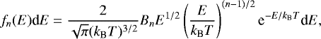 (1)
(1)
with
![Mathematical equation: \begin{equation*} \displaystyle B_{n}=\frac{\sqrt{\pi}}{2\mathrm\Gamma(n/2+1)}\quad \mbox{and}\quad n\in[1,+\infty]. \end{equation*}](/articles/aa/full_html/2018/08/aa32948-18/aa32948-18-eq2.png) (2)
(2)
and (Livadiotis & McComas 2009; Pierrard & Lazar 2010)
![Mathematical equation: \begin{equation*} f_{\kappa}(E)\textrm{d}E=\frac{2E^{1/2}}{\pi^{1/2}(k_{\textrm{B}}T)^{3/2}} \displaystyle A_{\kappa} \left[ 1+\frac{E}{(\kappa-3/2)k_{\textrm{B}}T}\right]^{-\kappa-1}\textrm{d}E, \end{equation*}](/articles/aa/full_html/2018/08/aa32948-18/aa32948-18-eq3.png) (3)
(3)
with
![Mathematical equation: \begin{equation*} A_{\kappa}=\frac{\mathrm\Gamma(\kappa+1)}{\mathrm\Gamma(\kappa-1/2)(\kappa-3/2)^{3/2}}\quad \mbox{and}\quad \kappa\in[3/2,+\infty], \end{equation*}](/articles/aa/full_html/2018/08/aa32948-18/aa32948-18-eq4.png) (4)
(4)
respectively. In these expressions E is the electron energy (eV), kB is the Boltzmann constant (erg K−1), T is the temperature (K), and Γ(x) is the Gamma function of variable x.
The n-distribution (which becomes the MB distribution when n = 1) is characterized by having a mean energy that depends on the n parameter being given by ⟨E⟩ = (3∕2)kBτ where τ = T(n + 2)∕3 is a pseudo-temperature. This means that at τ the mean energies of the n- and MB distributions are the same. Thus, τ has the same physical meaning as T in the MB distribution. The n-distributions with the same τ have their peaks higher and narrower than that of the MB distribution, that is, they have less electrons with both high and low energies, but have an increased number of electrons with intermediate energies (top panel of Fig. 1).
The κ-distribution is characterized by a high-energy power-law tail and having a mean energy that does not depend on κ and is given by ⟨E⟩ = 3∕2kBT. Hence, T can be defined as the thermodynamic temperature for these distributions. When κ → ∞, the MB distribution is recovered.As κ decreases, deviations from the MB distribution increase, reaching a maximum when κ approaches 3/2 (bottom panel of Fig. 1).
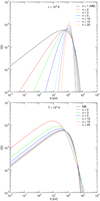 |
Fig. 1 Maxwell–Boltzmann (both panels), n (top panel) and κ (bottom panel) distributions at τ, T = 106 K. The n> 1 distributions have a steeper high-energy tail than the MB distribution. The κ distribution approaches MB when κ →∞. |
3 Internal energy and the adiabatic parameter γ
The internal energy of the gas parcel includes the contributions due to the thermal translational energy plus the energy stored in (or delivered) from the high ionization stages and from the excitation levels (see, e.g., Cox & Giuli 1968; Macfarlane 1989; Schmutzler & Tscharnuter 1993)
 (5)
(5)
with ρ, u, kB, and T denoting the gas density (g cm−3), the specific energy of the gas (erg g−1), respectively; ntot and ne are the total number density of the element with atomic number Z (hereafter referred to as element Z) and the electron density, respectively, and are given by
 (6)
(6)
where z is the ion state, and nZ and nZ,z are the number densities of the element Z and of its ionic state z. The energies stored in ionization and in excitation are, respectively,
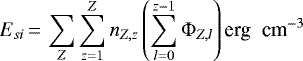 (7)
(7)
and
![Mathematical equation: \begin{equation*}E_{se}\,{=}\,\sum_{Z}\sum_{z=1}^{Z}\left[\sum_{j=n_{{o}}+1}n_{{Z,z,j}}\left(\mathrm\Delta E_{j,n_{{o}}}\right)_{{Z,z}}\right] \textrm{{erg\; cm}}^{-3}. \end{equation*}](/articles/aa/full_html/2018/08/aa32948-18/aa32948-18-eq8.png) (8)
(8)
In these equations ΦZ,l is the ionization potential (erg) of the ionization state l of the element Z and  is the excitation energy (erg) with respect to the ground level, no, of each ion. If the gas is to be ionized and excited then ρu erg cm−3 must be added to the gas. Of this amount Esi strips the atoms and ions of their electrons, Ese promotes the excitation of electrons in the atoms/ions and the reminder brings the system to a common temperature T.
The plasma pressure is
 (9)
(9)
where ⟨Z⟩ = ne∕ntot and μ are the mean electron charge and mean molecular weight, respectively. From Eqs. (5) and (9), it is seen that
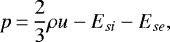 (10)
(10)
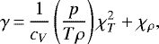
which is different than the classical relation p = (γ − 1)ρu (see, e.g., Vandenbroucke et al. 2013). Consequently, the adiabatic parameter 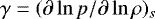 depends on the state of the plasma through the internal energy. It can be written as (Cox & Giuli 1968)
 (11)
(11)
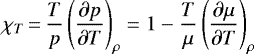
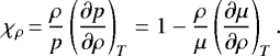
with  (erg g−1 K−1) denoting the specific heat at constant volume, and the coefficients χT and χρ (temperature and density exponents) are written in terms of μ as
 (12)
(12)
and
 (13)
(13)
4 Thermal model
In order to study the evolution of γ with temperature, we follow the evolution of a gas parcel freely cooling from 109 K (where it is assumed to be completely ionized) evolving in CIE. The gas parcel is composed of the ten most abundant elements in Nature (H, He, C, N, O, Ne, Mg, Si, S, and Fe) having solar abundances. These are based on Asplund et al. (2009) and include the updates to the Mg, Si, S, and Fe abundances by Scott et al. (2015b,a; see also Amarsi & Asplund 2017 for the abundance of Si). The physical processes included in these calculations comprise electron impact ionization (including excitation–autoionization), radiative and dielectronic recombinations and line excitation by electrons assuming the coronal approximation. In these calculations line excitation/deexcitation by protons, continuum emission, and charge exchange reactions are not included.
4.1 Ionic fractions
The time-independent evolution of the ion fractions due to the 102 ions and 10 atoms (in a total of 112 equations) where ionization and recombinations of ions of nuclear charge Z occur between neighbouring ionization stages z − 1, z, and z + 1, is given by
 (14)
(14)
where  and
and  are the rates of recombination and ionization from state (Z, z) to (Z, z − 1) and (Z, z + 1), respectively; ne is the electron density and xZ,z = nZ,z∕nZ the ionic fraction of element Z with effective charge z. The ion density is then given by
 (15)
(15)
with A(Z) = nZ∕nH and nH being the abundance of element Z and the hydrogen density. The system of equations can be cast into the matrix equation
 (16)
(16)
where X is a vector comprising all ion fractions xZ,z and A is a tridiagonal matrix with elements  ,
,  , and
, and  at each row populating the diagonal band.
4.2 Ionization and recombination rates
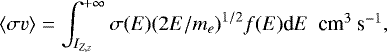
From the electron impact ionization cross sections, we calculate the corresponding ionization rates associated with an ion of atomic number Z and ionic charge z by averaging the product σ(E)v over the impacting particle kinetic energy distribution f(E):
 (17)
(17)
where me is the electron mass, and IZ,z is the threshold energy in eV.
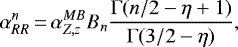
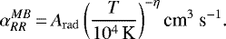
The radiative and dielectronic recombination rates for the n distribution are calculated from the fit coefficients to the Maxwellian rates (Dzifčáková 1998), that is, the radiative recombination rates for the n-distribution are determined from
 (18)
(18)
where  is the Maxwellian radiative recombination rate, and η is a parameter of the power-law fit of the Maxwellian rate (Woods et al. 1981):
 (19)
(19)
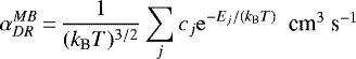
The dielectronic recombination rates for the n-distribution of electrons are determined from coefficients of the Maxwellian rates given by the Burgess (1965) general formula
 (20)
(20)
through (Dzifčáková 1998):
 (21)
(21)
In these expressions Arad and cj are fitting coefficients.
The radiative and dielectronic recombination rates for the κ distribution are also based on the Maxwellian rates and are expressed, respectively, by (Wannawichian et al. 2003; Dzifčáková & Dudík 2013; see also Dzifčáková 1992)
 (22)
(22)
and
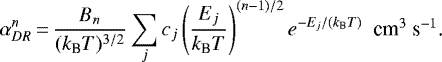
![Mathematical equation: \begin{equation*} \alpha_{DR}^{\kappa}\,{=}\,\frac{A_{\kappa}}{(k_{\textrm{B}}T)^{3/2}}\sum_{j}c_{j}\left[1+\frac{E_{j}}{(\kappa-3/2)k_{\textrm{B}}T}\right]^{-(\kappa+1)} \mbox{~~cm$^{3}$ s$^{-1}$}, \end{equation*}](/articles/aa/full_html/2018/08/aa32948-18/aa32948-18-eq32.png) (23)
(23)
4.3 Levels populations and excitation rates
The levels populations are calculated assuming excitation–deexcitation equilibrium, that is, equilibrium between the excitations (by particle impact) and deexcitations (by particle impact and spontaneous decays) to and from a level. We assume that the excitations and deexcitations by particle impact are only due to electrons. The population of level j is determined from the collisional excitations of electrons from levels m to level j (m < j; excitation rate  ) and from level j to levels n (j < n; excitation rate
  ), and deexcitations from levels n to level j (n > j; collisional deexcitation rates
  and spontaneous decay rates Anj) and from level j to levels m (j > m; collisional deexcitation and spontaneous decay rates
  and Ajm, respectively). The ground level is populated/depopulated by the deexcitations/excitations from/to levels above it. Thus, the population of a level j is given by thesolution of (Phillips et al. 2008)
![Mathematical equation: \begin{eqnarray*}&& \sum_{m<j}C_{mj}^{e}n_{{e}}n_{Z,z,m}+\sum_{n>j}\left(A_{nj}+C_{nj}^{d}n_{e}\right)n_{Z,z,n} \nonumber \\ &&\qquad -n_{Z,z,j}\left[\sum_{j<n}C_{jn}^{e}n_{e}+\sum_{j>m}\left(A_{jm}+C_{jm}^{d}n_{e}\right)\right] = 0, \end{eqnarray*}](/articles/aa/full_html/2018/08/aa32948-18/aa32948-18-eq37.png) (24)
(24)
coupled to the equation of mass conservation
 (25)
(25)
In these equations nZ,z,m, nZ,z,j, nZ,z,n denote the population densities (in units of cm−3) of levels m, j, and n, respectively; ne and nZ,z are the electron and ion densities. The units of the excitation/deexcitation rates are in cm3 s−1, while those of the spontaneous decay rates are in s−1.
The rates of collisional excitation from level i to level j (i < j) and deexcitation from level j to level i are determined by the average of the corresponding cross sections (σij(Ee) and  ) over all possible velocities of the incident electrons, that is,
  and
and 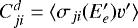 , respectively.The excitation cross section can be written in terms of the dimensionless collision strength Ωij through the expressions
 (26)
(26)
where a0 is the Bohr radius, EH is the ground state energy of the hydrogen atom, Ee is the energy of the incident electron, ωi is the statistical weight of levels i and j, Eij is the excitation energy between levels i, and U = Ee∕Eij is the reduced electron energy. The collision strength is symmetrical with respect to the direct and the inverse processes, that is,  . Therefore, the deexcitation cross section can be written as
 (27)
(27)
In this expression ωj is the statistical weight of level j,  is the energy of the electron impacting on the electrons in level j and
 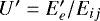 is the reduced electron energy.
For electrons with a MB, κ and n distributions, the rates of collisional excitation between levels i and j and deexcitation between levels j and i are given by (see, for example, Dudík et al. 2014)
 (28)
(28)
and
 (29)
(29)
respectively. In these expressions y = Eij∕kBT, ωi and ωj are the statistical weights of levels i and j, respectively, and T is the temperature (in degrees K). The Υij(T) (also known as the effective collision strength or Upsilon) and Υji(T) (also known as Downsilon) have different forms according to the electron distribution. They are given by
 (30)–(35)
for thermal,
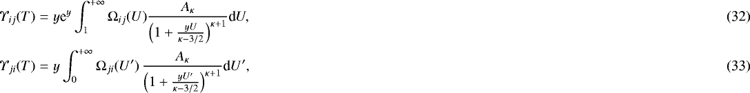
for κ, and

for n distributed electrons. It should be noticed from the above expressions that Υij (T)≠Υji(T) for the non-Maxwellian distributions.
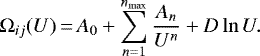
Ωij(U) can be written with the functional (Mewe 1972; Mewe & Gronenschild 1981; Clark et al. 1982; Suno & Kato 2006; Dzifčáková 2006; Dzifčáková et al. 2015)
 (36)
(36)
Making use of the exponential integral of order n, En (y) (Abramowitz & Stegun 1972)1, the integral in the RHS of (30) becomes
![Mathematical equation: \begin{eqnarray*}\int_{1}^{\infty} \mathrm\Omega_{ij}(U)\, \textrm{e}^{-yU}\textrm{d}U &= &\int_{1}^{\infty} \left[A_{0}+\sum_{n=1}^{n_{\textrm{{max}}}}\frac{A_{n}}{U^{n}}+D\ln U\right]\,\textrm{e}^{-yU}\textrm{d}U \nonumber \\ &=& A_{0}\frac{e^{-y}}{y}+\sum_{n=1}^{n_{\textrm{{max}}}}\left[A_{n}E_{n}(y)\right]+\frac{D}{y}E_{1}(y), \end{eqnarray*}](/articles/aa/full_html/2018/08/aa32948-18/aa32948-18-eq53.png) (39)
(39)
and Υij is given by
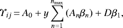 (40)
(40)
with βn = eyEn(y). We can use this result to fit the available Υij and thus obtain the corresponding collision strength through the determination of the best-fit parameters A0,...,  and D (Dzifčáková 2006; Dzifčáková et al. 2015). This procedure is used because most of the theoretical collision strengths are not made available by their authors, instead what is available are the effective collision strengths calculated with the MB distribution.
In the present calculations we assumed an atomic/ionic model composed of 30 levels and used the procedure discussed above with nmax = 8 to determine the collision strengths of the transitions (see further details in de Avillez & Anela, in prep.).
4.4 Atomic data
Electron impact ionization cross sections discussed in Dere (2007) and available in the Chianti database (see, e.g., Dere et al. 2009)are adopted.
The Maxwellian radiative recombination rate coefficients are taken from Badnell (2006c)2 for all bare nuclei through Na-like ions recombining to H through Mg-like ions, Altun et al. (2007) for Mg-like ions, Abdel-Naby et al. (2012) for Al-like ions, Nikolić et al. (2010) for Ar-like ions, and Badnell (2006b) for FeXiii–FeX ions. The Maxwellian dielectronic recombination rates are taken from Badnell (2006a) or H-like ions, Bautista & Badnell (2007) for He-like ions, Colgan et al. (2003, 2004) for Li and Be-like ions, Altun et al. (2004, 2006, 2007) for B, Na, and Mg-like ions, Zatsarinny et al. (2003, 2004a,b, 2006) for C, O, F, and Ne-like ions, Mitnik & Badnell (2004) for N-like ions, Abdel-Naby et al. (2012) for Al-like ions, and Nikolić et al. (2010) for Ar-like ions. We further used the data in the errata by Altun et al. (2005) for NeVi and MgVii, Zatsarinny et al. (2005a) for NIi, and Zatsarinny et al. (2005b) for NeIii, MgV, and FeXix.
Radiative and dielectronic recombination rates for SIi, SIii, and FeVii are adopted from Mazzotta et al. (1998), while for the remaining ions we adopt the radiative and dielectronic recombination rates derived with the unified electron-ion recombination method (Nahar & Pradhan 1994) and available at NORAD-Atomic-Data3.
The wavelengths, Einstein coefficients of spontaneous transitions and the effective collision strengths of transitions calculated for a MB electron distributions are taken from version 8.0.7 of the CHIANTI atomic database4 (Del Zanna et al. 2015).
4.5 Numerical methods and calculations
The ionic structure of the plasma is determined by solving the system of Eq. (14) at each temperature using a Gauss elimination method with scaled partial pivoting (Cheney & Kincaid 2008) and a tolerance of 10−15. The numerical integrations in Eq. (17) are carried out with a precision of 10−15 using the double-exponential over a semi-finite interval method of Takahasi & Mori (1974) and Mori & Sugihara (2001). We use a modified version (parallelized version) of the Numerical Automatic Integrator for Improper Integral package developed by T. Ooura5.
The calculations proceed as follows: follow the evolution of a gas parcel freely evolving isochorically under CIE from the initial conditions (fully ionized plasma at 109 K with a density nH = 1.0 cm−3). At each temperature the electron density, ionization and recombination rates and the ionic fractions are determined first. This is followed by the determination of the collisional excitation rates and of the populations of the excited states given by Eq. (24). Finally, the mean molecular weight, the pressure, the internal energy, the specific heat at constant volume cv and the gamma parameter are calculated.
5 Results
5.1 Internal energy
The total specific internal energy (erg g−1) of a plasma evolving under CIE for the MB, n and κ distributions, using n, κ = 2, 3, 5, 10, and 15 are displayed in Fig. 2, while its thermal and ionization components are shown in Fig. 3. The excitation component of the internal energy has less than a percent contribution to the total energy and thus, is not shown in the figures. The top and bottom panels in both figures refer to plasmas with, respectively, n and κ electron distributions. Maxwellian energies are shown by the black lines and dots in the top and bottom panels of both figures.
The total internal energy (as well as the thermal, ionization, and excitation components) of the gas varies according to the parameters κ and n. As κ increases (n increases), the internal energy approaches (moves away of) that obtained for a Maxwellian distribution of electrons. The largest variations in the total internal energy occur in κ distributed plasmas and are mainly driven by the large variations (more than an order of magnitude with regard the thermal component for T <104 K) in the ionization energy. In n distributed plasmas the energies (total, thermal and ionization) profiles are similar but with a shift to the left as n increases (top panels of both figures). In the n-distributed plasma the dominance of the ionization energy over the thermal component only occurs down to the temperature at which the ionization energy has a sharp decrease. Below that temperature the thermal energy dominates (top panel of Fig. 3).
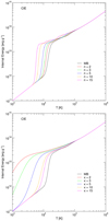 |
Fig. 2 Total specific internal energy of the plasma for Maxwell–Boltzmann (black line in both panels), n (top panel), and κ (bottom panel) distributions calculated for n, κ = 2, …, 15. |
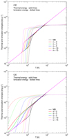 |
Fig. 3 Specific thermal and ionization energies of the plasma for Maxwell–Boltzmann (black solid and dashed lines in both panels), n (top panel), and κ (bottom panel) distributions with n, κ = 2, …, 15. |
5.2 The adiabatic parameter
Figure 4 displays the γ parameter calculated for a monoatomic Maxwellian plasma composed of (1) H (black line), (2) H and He (red line), (3) metals (C, N, O, Ne, Mg, Si, S, and Fe; green line), and (4) all elements (H, He, and metals; black dashed line). The adiabatic parameter is 5/3 at T ≤8000 K (cases 1, 2, and 4), at T ≤ 3090 K (case 3) and at T ≥ 5 × 10⁴ K (case 1), 2 × 10⁵ K (case 2), 5 × 10⁶ K (case 4), and 4 × 10⁸ K (case 3). In the remaining temperatures, γ has substantial variations having values as low as 1.08 (cases 1, 2, and 4) and 1.1 (case 3). In the mixtures comprising H, He, and metals the former two determine the value of γ as they haveabundances much larger than the remaining elements. Thus, the three transitions observed in case (4) are determined from left to right (from low to high temperatures) by the HI, HeI, and HeIi ionizations, respectively. In case (3) the observed transitions in the γ profile are due to the ionization of the most abundant elements among the metals.
Figure 5 displays the temperature variation of the adiabatic parameter in plasmas with n (top and middle panels) and κ (bottom panel) electron distributions and composed of a mixture of H, He, and metals (case 4) for n, κ = 2, …, 15. The Maxwellian evolution of γ is shown by the black dashed lines. As n increases, γ moves towards the left of the Maxwellian value with the same number of transitions (a result of the dominance of the ionization by H and He due to their abundances) but shifted to lower temperatures than those observed for lower n. The local minimum seen after each transition becomes deeper with increasing n. Therefore, the minimum value of γ decreases from 1.09 for the Maxwellian distributed plasma to 1.025 for n = 15 passing by 1.05 for n = 5. That is, with increasing n, the plasma behaves almost isothermally at that range for temperatures.
In a κ distributed plasma, as κ increases γ approaches the Maxwellian value (bottom panel of Fig. 5). While the Maxwellian γ has three transitions, the κ distributed γ only has three transitions for κ > 15. Over the remaining values of κ two transitions are seen for κ > 4 and no transitions are seen at lower κ. The latter is a consequence of the early ionization of H and He when κ has small values as can be seen in Fig. 6, which displays the ionization rates of H, He, and He+, thereby affecting the internal energy of the plasma. As κ increases, the minimum value of γ increases from almost 1.01 (κ = 2) to 1.09 as κ →∞, that is, the Maxwellian value. γ = 5∕3 at T > 2 × 10⁵ K for all possible values of κ, while at T < 8000 K γ < 5∕3 for κ < 7.
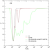 |
Fig. 4 Evolution of the γ parameter in different plasmas composed only of H (black line), H and He (red line), metals (C, N, O, Ne, Mg, Si, S, and Fe; green line), and all elements (black dashed line). Note that H and He determine the evolution of γ for the calculations involving all the ten elements because the abundances of the metals are much smaller than those of H and He. |
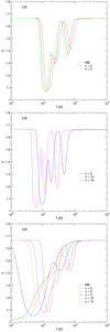 |
Fig. 5 Evolution with temperature of the adiabatic parameter (γ) of a plasma evolving under CIE for Maxwell–Boltzmann (black line in the top and bottom panels), n (top and middle panels), and κ (bottom panel), distributions calculated for n, κ = 2, 3, 5, 10, and 15. |
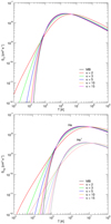 |
Fig. 6 Variation with κ of the ionization rates of H, He, and He+. |
6 Final remarks
The calculations presented in this paper comprise the determination of the γ parameter in a plasma characterized by MB, n and κ electron distributions and evolving under collisional ionization equilibrium and cooling from 109 K. Two particle processes (electron impact ionization including excitation–autoionization, radiative and dielectronic recombination and excitation) are considered in all the calculations. The populations of excited states are calculated assuming the coronal approximation. It is shown that the γ parameter in an optically thin monoatomic plasma depends on its ionic state and most importantly on the contribution of the ionization energy to the total internal energy. The excitation energy has a negligible contribution to the total internal energy. Lookup tables of the temperature variation of γ are provided as supplementary material and can be used in simulations of solar, interstellar or intergalactic plasmas.
Although CIE cooling functions are widely used in interstellar medium simulations, caution should be exercised as CIE is only valid provided the cooling timescale (τcool) of the plasma is larger than the recombination time scales of the different ions ( ), something that typically occurs at T > 106 K. For lower temperatures,
  , and therefore, cooling and recombination are not synchronized, and the plasma appears overionized, if it is cooling (for detailed discussions, see, e.g., Kafatos 1973; Shapiro & Moore 1976; Sutherland & Dopita 1993; Schmutzler & Tscharnuter 1993; Gnat & Sternberg 2007; de Avillez & Breitschwerdt 2010, and references therein). Consequently, the history of each gas parcel, evolving from different initial conditions, will have different ionic/radiative histories. Something that does not happen with CIE.
Futhermore, de Avillez & Breitschwerdt (2012) have shown in a muti-fluid time-dependent study of the dynamical and thermal evolutions of the interstellar gas6 that this historyreflects the feedback between heating, cooling and the dynamics of the system. Therefore, even with the same initial conditions the gas parcels will have a different ionic/radiative history with the corresponding emissivities having an order of magnitude differences.
We have shown that widely performed hydro- and magnetohydrodynamical simulations of optically thin plasmas like in the interstellar and intergalactic medium should take into account not only the time-dependent ionization structure (see de Avillez & Breitschwerdt 2012) but also the detailed distribution between internal and potential energies leading to different values of the ratio of specific heats, γ. In addition, it should be checked during simulations if MB equilibrium is established or if more generalized forms of electron distributions like κ or n are more applicable.
In a forthcoming paper, we describe the evolution of the γ parameter under non-equilibrium ionization conditions and with molecular contributions to the ionization state of the plasma as they affect the γ parameter at low temperatures (see, e.g., Decampli et al. 1978; Wuchterl 1991; D’Angelo & Bodenheimer 2013).
Acknowledgements
We thank the anonymous referee for the comments improving the paper. This research was supported by the project Enabling Green E-science for the SKA Research Infrastructure (ENGAGE SKA), reference POCI-01-0145-FEDER-022217, funded by COMPETE 2020 and FCT, Portugal. D.B. acknowledges support from the DeutscheForschungsgemeinschaft, DFG project ISM–SPP 1573. The calculations were carried out at the ISM – Xeon Phi cluster of the Computational Astrophysics Group, University of Évora, acquired under project “Hybrid computing using accelerators & coprocessors-modelling nature with a novell approach” (PI: M.A.), InAlentejo program, CCDRA, Portugal.
Appendix A Tables at the CDS
In the supplementary material, Tables (1 and 2) referring to the adiabatic parameter of the gas versus temperature (K) for the Maxwellian, n and κ distributions, with n, κ = 2, 3, 5, 10, 15 and 25, are provided. We note that n = 1 corresponds to the Maxwellian distribution. More data can be provided by the corresponding author upon request.
References
- Abdel-Naby, S. A., Nikolić, D., Gorczyca, T. W., Korista, K. T., & Badnell, N. R. 2012, A&A, 537, A40 [NASA ADS] [CrossRef] [EDP Sciences] [Google Scholar]
- Abramowitz, M., & Stegun, I. A. 1972, Handbook of Mathematical Functions (New York: Dover Publications, Inc.) [Google Scholar]
- Altun, Z., Yumak, A., Badnell, N. R., Colgan, J., & Pindzola, M. S. 2004, A&A, 420, 775 [NASA ADS] [CrossRef] [EDP Sciences] [Google Scholar]
- Altun, Z., Yumak, A., Badnell, N. R., Colgan, J., & Pindzola, M. S. 2005, A&A, 433, 395 [NASA ADS] [CrossRef] [EDP Sciences] [Google Scholar]
- Altun, Z., Yumak, A., Badnell, N. R., Loch, S. D., & Pindzola, M. S. 2006, A&A, 447, 1165 [NASA ADS] [CrossRef] [EDP Sciences] [Google Scholar]
- Altun, Z., Yumak, A., Yavuz, I., et al. 2007, A&A, 474, 1051 [NASA ADS] [CrossRef] [EDP Sciences] [Google Scholar]
- Amarsi, A. M., & Asplund, M. 2017, MNRAS, 464, 264 [NASA ADS] [CrossRef] [Google Scholar]
- Asplund, M., Grevesse, N., Sauval, A. J., & Scott, P. 2009, ARA&A, 47, 481 [NASA ADS] [CrossRef] [Google Scholar]
- Badnell, N. R. 2006a, A&A, 447, 389 [NASA ADS] [CrossRef] [EDP Sciences] [Google Scholar]
- Badnell, N. R. 2006b, ApJ, 651, L73 [NASA ADS] [CrossRef] [Google Scholar]
- Badnell, N. R. 2006c, ApJS, 167, 334 [NASA ADS] [CrossRef] [Google Scholar]
- Bautista, M. A., & Badnell, N. R. 2007, A&A, 466, 755 [NASA ADS] [CrossRef] [EDP Sciences] [Google Scholar]
- Behringer, K., & Fantz, U. 1994, J. Phys. D, 27, 2128 [NASA ADS] [CrossRef] [Google Scholar]
- Berezhko, E. G. & Ellison, D. C. 1999, ApJ, 526, 385 [NASA ADS] [CrossRef] [Google Scholar]
- Burgess, A. 1965, ApJ, 141, 1588 [NASA ADS] [CrossRef] [Google Scholar]
- Cheney, W., & Kincaid, D. 2008, Numerical Mathematics and Computing, 6th edn. (Belmont: Thomson Brooks/Cole) [Google Scholar]
- Clark, R. E. H., Magee, Jr., N. H., Mann, J. B., & Merts, A. L. 1982, ApJ, 254, 412 [NASA ADS] [CrossRef] [Google Scholar]
- Colgan, J., Pindzola, M. S., Whiteford, A. D., & Badnell, N. R. 2003, A&A, 412, 597 [NASA ADS] [CrossRef] [EDP Sciences] [Google Scholar]
- Colgan, J., Pindzola, M. S., & Badnell, N. R. 2004, A&A, 417, 1183 [NASA ADS] [CrossRef] [EDP Sciences] [Google Scholar]
- Cox, J. P., & Giuli, R. T. 1968, Principles of Stellar Structure, vol. 1 (Gordon and Breach Science Pub.) [Google Scholar]
- D’Angelo, G., & Bodenheimer, P. 2013, ApJ, 778, 77 [NASA ADS] [CrossRef] [Google Scholar]
- de Avillez, M. A. & Breitschwerdt, D. 2010, ASP Conf. Ser., 438, 313 [Google Scholar]
- de Avillez, M. A., & Breitschwerdt, D. 2012, ApJ, 756, L3 [NASA ADS] [CrossRef] [Google Scholar]
- de Avillez, M. A., & Breitschwerdt, D. 2015, A&A, 580, A124 [NASA ADS] [CrossRef] [EDP Sciences] [Google Scholar]
- de Avillez, M. A., & Breitschwerdt, D. 2017, ApJS, 232, 12 [NASA ADS] [CrossRef] [Google Scholar]
- Decampli, W. M., Cameron, A. G. W., Bodenheimer, P., & Black, D. C. 1978, ApJ, 223, 854 [NASA ADS] [CrossRef] [Google Scholar]
- Del Zanna, G., Dere, K. P., Young, P. R., Landi, E., & Mason, H. E. 2015, A&A, 582, A56 [NASA ADS] [CrossRef] [EDP Sciences] [Google Scholar]
- Dere, K. P. 2007, A&A, 466, 771 [NASA ADS] [CrossRef] [EDP Sciences] [Google Scholar]
- Dere, K. P., Landi, E., Young, P. R., et al. 2009, A&A, 498, 915 [NASA ADS] [CrossRef] [EDP Sciences] [Google Scholar]
- Druyvesteyn, M. J. 1930, Z. Phys., 64, 781 [NASA ADS] [CrossRef] [Google Scholar]
- Dudík, J., Del Zanna, G., Mason, H. E., & Dzifčáková E. 2014, A&A, 570, A124 [NASA ADS] [CrossRef] [EDP Sciences] [Google Scholar]
- Dzifčáková, E. 1992, Sol. Phys., 140, 247 [NASA ADS] [CrossRef] [Google Scholar]
- Dzifčáková, E. 1998, Sol. Phys., 178, 317 [NASA ADS] [CrossRef] [Google Scholar]
- Dzifčáková, E. 2006, Sol. Phys., 234, 243 [NASA ADS] [CrossRef] [Google Scholar]
- Dzifčáková, E., & Dudík, J. 2013, ApJS, 206, 6 [NASA ADS] [CrossRef] [Google Scholar]
- Dzifčáková, E., Homola, M., & Dudík, J. 2011, A&A, 531, A111 [NASA ADS] [CrossRef] [EDP Sciences] [Google Scholar]
- Dzifčáková, E., Dudík, J., Kotrč, P., Fárník, F., & Zemanová, A. 2015, ApJS, 217, 14 [NASA ADS] [CrossRef] [Google Scholar]
- Gnat, O., & Sternberg, A. 2007, ApJS, 168, 213 [NASA ADS] [CrossRef] [Google Scholar]
- Hares, J. D., Kilkenny, J. D., Key, M. H., & Lunney, J. G. 1979, Phys. Rev. Lett., 42, 1216 [NASA ADS] [CrossRef] [Google Scholar]
- Humphrey, A., & Binette, L. 2014, MNRAS, 442, 753 [NASA ADS] [CrossRef] [Google Scholar]
- Kafatos, M. 1973, ApJ, 182, 433 [NASA ADS] [CrossRef] [Google Scholar]
- Karlický, M., Dzifčáková, E., & Dudík, J. 2012, A&A, 537, A36 [NASA ADS] [CrossRef] [EDP Sciences] [Google Scholar]
- Livadiotis, G., & McComas, D. J. 2009, J. Geophys. Res., 114, A11105 [NASA ADS] [CrossRef] [Google Scholar]
- Macfarlane, J. J. 1989, Comput. Phys. Commun., 56, 259 [NASA ADS] [CrossRef] [Google Scholar]
- Mazzotta, P., Mazzitelli, G., Colafrancesco, S., & Vittorio, N. 1998, A&AS, 133, 403 [NASA ADS] [CrossRef] [EDP Sciences] [Google Scholar]
- Mewe, R. 1972, A&A, 20, 215 [NASA ADS] [Google Scholar]
- Mewe, R., & Gronenschild, E. H. B. M. 1981, A&AS, 45, 11 [NASA ADS] [Google Scholar]
- Mitnik, D. M. & Badnell, N. R. 2004, A&A, 425, 1153 [NASA ADS] [CrossRef] [EDP Sciences] [Google Scholar]
- Mori, M. & Sugihara, M. 2001, J. Comput. Appl. Math., 127, 287 [NASA ADS] [CrossRef] [Google Scholar]
- Nahar, S. N. & Pradhan, A. K. 1994, Phys. Rev. A, 49, 1816 [NASA ADS] [CrossRef] [PubMed] [Google Scholar]
- Nicholls, D. C., Dopita, M. A., Sutherland, R. S., Kewley, L. J., & Palay, E. 2013, ApJS, 207, 21 [NASA ADS] [CrossRef] [Google Scholar]
- Nikolić, D., Gorczyca, T. W., Korista, K. T., & Badnell, N. R. 2010, A&A, 516, A97 [NASA ADS] [CrossRef] [EDP Sciences] [Google Scholar]
- Phillips, K. J. H., Feldman, U., & Landi, E. 2008, Ultraviolet and X-ray Spectroscopy of the Solar Atmosphere (Cambridge: Cambridge University Press) [CrossRef] [Google Scholar]
- Pierrard, V., & Lazar, M. 2010, Sol. Phys., 267, 153 [NASA ADS] [CrossRef] [Google Scholar]
- Porquet, D., Arnaud, M., & Decourchelle, A. 2001, A&A, 373, 1110 [NASA ADS] [CrossRef] [EDP Sciences] [Google Scholar]
- Schmutzler, T., & Tscharnuter, W. M. 1993, A&A, 273, 318 [NASA ADS] [Google Scholar]
- Scott, P., Asplund, M., Grevesse, N., Bergemann, M., & Sauval, A. J. 2015a, A&A, 573, A26 [NASA ADS] [CrossRef] [EDP Sciences] [Google Scholar]
- Scott, P., Grevesse, N., Asplund, M., et al. 2015b, A&A, 573, A25 [NASA ADS] [CrossRef] [EDP Sciences] [Google Scholar]
- Seely, J. F., Feldman, U., & Doschek, G. A. 1987, ApJ, 319, 541 [NASA ADS] [CrossRef] [Google Scholar]
- Shapiro, P. R.& Moore, R. T. 1976, ApJ, 207, 460 [NASA ADS] [CrossRef] [Google Scholar]
- Suno, H., & Kato, T. 2006, Atomic Data and Nuclear Data Tables, 92, 407 [Google Scholar]
- Sutherland, R. S. & Dopita, M. A. 1993, ApJS, 88, 253 [NASA ADS] [CrossRef] [Google Scholar]
- Takahasi, H., & Mori, M. 1974, Pub. Res. Inst. Math. Sci., 9, 721 [Google Scholar]
- Vaidya, B., Mignone, A., Bodo, G., & Massaglia, S. 2015, A&A, 580, A110 [NASA ADS] [CrossRef] [EDP Sciences] [Google Scholar]
- Vandenbroucke, B., De Rijcke, S., Schroyen, J., & Jachowicz, N. 2013, ApJ, 771, 36 [NASA ADS] [CrossRef] [Google Scholar]
- Vasyliunas, V. M. 1968, Astrophys. Space Sci. Lib., 10, 622 [Google Scholar]
- Wannawichian, S., Ruffolo, D., & Kartavykh, Y. Y. 2003, ApJS, 146, 443 [NASA ADS] [CrossRef] [Google Scholar]
- Woods, D. T., Shull, J. M., & Sarazin, C. L. 1981, ApJ, 249, 399 [NASA ADS] [CrossRef] [Google Scholar]
- Wuchterl, G. 1990, A&A, 238, 83 [NASA ADS] [Google Scholar]
- Wuchterl, G. 1991, Icarus, 91, 39 [NASA ADS] [CrossRef] [Google Scholar]
- Zatsarinny, O., Gorczyca, T. W., Korista, K. T., Badnell, N. R., & Savin, D. W. 2003, A&A, 412, 587 [NASA ADS] [CrossRef] [EDP Sciences] [Google Scholar]
- Zatsarinny, O., Gorczyca, T. W., Korista, K. T., Badnell, N. R., & Savin, D. W. 2004a, A&A, 417, 1173 [NASA ADS] [CrossRef] [EDP Sciences] [Google Scholar]
- Zatsarinny, O., Gorczyca, T. W., Korista, K. T., Badnell, N. R., & Savin, D. W. 2004b, A&A, 426, 699 [NASA ADS] [CrossRef] [EDP Sciences] [Google Scholar]
- Zatsarinny, O., Gorczyca, T. W., Korista, K. T., et al. 2005a, A&A, 440, 1203 [NASA ADS] [CrossRef] [EDP Sciences] [Google Scholar]
- Zatsarinny, O., Gorczyca, T. W., Korista, K. T., et al. 2005b, A&A, 438, 743 [NASA ADS] [CrossRef] [EDP Sciences] [Google Scholar]
- Zatsarinny, O., Gorczyca, T. W., Fu, J., et al. 2006, A&A, 447, 379 [NASA ADS] [CrossRef] [EDP Sciences] [Google Scholar]
The exponential integral of order n is
 (37)
(37)
En+1 (y) can be determined through the recurrence formula
 (38)
(38)
Hydrodynamical multi-fluid simulations of the interstellar medium in the disk and halo of the Milky Way, including the time-dependent evolution of all atoms and ions associated with the ten most abundant elements in Nature (H, He, C, N, O, Ne, Mg, Si, S, and Fe).
All Figures
|
Fig. 1 Maxwell–Boltzmann (both panels), n (top panel) and κ (bottom panel) distributions at τ, T = 106 K. The n> 1 distributions have a steeper high-energy tail than the MB distribution. The κ distribution approaches MB when κ →∞. |
| In the text | |
|
Fig. 2 Total specific internal energy of the plasma for Maxwell–Boltzmann (black line in both panels), n (top panel), and κ (bottom panel) distributions calculated for n, κ = 2, …, 15. |
| In the text | |
|
Fig. 3 Specific thermal and ionization energies of the plasma for Maxwell–Boltzmann (black solid and dashed lines in both panels), n (top panel), and κ (bottom panel) distributions with n, κ = 2, …, 15. |
| In the text | |
|
Fig. 4 Evolution of the γ parameter in different plasmas composed only of H (black line), H and He (red line), metals (C, N, O, Ne, Mg, Si, S, and Fe; green line), and all elements (black dashed line). Note that H and He determine the evolution of γ for the calculations involving all the ten elements because the abundances of the metals are much smaller than those of H and He. |
| In the text | |
|
Fig. 5 Evolution with temperature of the adiabatic parameter (γ) of a plasma evolving under CIE for Maxwell–Boltzmann (black line in the top and bottom panels), n (top and middle panels), and κ (bottom panel), distributions calculated for n, κ = 2, 3, 5, 10, and 15. |
| In the text | |
|
Fig. 6 Variation with κ of the ionization rates of H, He, and He+. |
| In the text | |
Current usage metrics show cumulative count of Article Views (full-text article views including HTML views, PDF and ePub downloads, according to the available data) and Abstracts Views on Vision4Press platform.
Data correspond to usage on the plateform after 2015. The current usage metrics is available 48-96 hours after online publication and is updated daily on week days.
Initial download of the metrics may take a while.