© ESO 2018

1 Introduction

The magnetic Rayleigh–Taylor (MRT) instability occurs in many astrophysical systems. Examples include shells of young supernova remnants (Jun et al. 1995), the interface between an expanding pulsar wind nebula and its surrounding supernova remnant (Bucciantini et al. 2004), and the optical filaments observed in the Crab nebula (Stone & Gardiner 2007).

The MRT instability is also very important in applications to solar and heliospheric physics. For example, Isobe et al. (2005, 2006) suggested that the MRT instability is responsible for the filamentary structure in mass and current density in the emerging flux regions. Ryutova et al. (2010) conjectured that dynamical processes taking place in prominences are caused by the MRT instabilities. Hillier et al. (2011, 2012a,b) carried out three-dimensional magnetohydrodynamic simulations to study the non-linear evolution of the Kippenhahn–Schluter prominence model which is caused by the MRT instability. Recently, Carlyle & Hillier (2017) studied the magnetic field effect on the non-linear development of the MRT instability. Terradas et al. (2012) proposed that the MRT instability is responsible for short lifetimes of magnetic threads in solar prominences. Díaz et al. (2012, 2014) and Ruderman et al. (2017) investigated the MRT instabilities in partially ionised plasmas with the application to solar prominences.

Studying the MRT instability is also important for understanding physical processes in the region of interaction of the solar wind and the local interstellar medium called the heliospheric interface. The generally accepted model of this interaction is the model with two shocks that was first developed by Baranov et al. (1971; for the latest progress, see the review papers by Baranov 2009a,b and Pogorelov et al. 2017a). In this model, the supersonic solar wind flow compressed at the termination shock, and the supersonic interstellar medium flow compressed at the bow shock are separated by a tangential discontinuity called the heliopause. To our knowledge, Fahr et al. (1986) were the first to address the heliopause stability problem. After that the heliopause stability problem received much attention with the main emphasis on the Kelvin–Helmholtz (KH) instability (e.g. Baranov et al. 1992; Ruderman & Fahr 1993,1995; Chalov 1994; see also the review articles by Ruderman & Belov 2010; Taroyan & Ruderman 2011). However, the MRT instability also can operate at the heliopause. Liewer et al. (1996), Florinski et al. (2005), and Borovikov et al. (2008) studied the Rayleigh–Taylor instability of the heliopause caused by change exchange (see also Pogorelov et al. 2017b and review by Pogorelov et al. 2017a). This instability can also be caused by the increase in the solar wind dynamic pressure during the solar cycle. The pressure increase pushes the interaction region of the solar wind and interstellar medium in the anti-solar direction causing its acceleration. This acceleration can act as an effective gravity.

Terradas et al. (2012) studied the MRT instability of a horizontal slab filled in with dense plasma surrounded by rarefied plasma. They assumed that the magnetic field had the same direction everywhere. As a result, they obtained that the initial-value problem is ill posed because the increment of perturbations with the wavevector perpendicular to the background magnetic field is unbounded. Ruderman et al. (2014) extended this study to include magnetic shear. They obtained in this case that the instability increment is bounded and the initial-value problem is well posed. BothTerradas et al. (2012) and Ruderman et al. (2014) used the approximation of incompressible plasma. Ruderman (2017) generalised their analysis to include the plasma compressibility.

Ruderman (2015) estimated the characteristic growth time of the MRT instability at the heliopause and found that it is comparable with the solar cycle period. This implies that we cannot assume that the effective gravity caused by the heliospheric interface acceleration is constant. Rather we have to consider the oscillating acceleration. The aim of this article is to study this problem. It is organised as follows. In the next section, we formulate the problem and write down the governing equations and boundary conditions. In Sect. 3 we derive the equation describing the magnetic interface oscillation amplitude. In Sect. 4 we study the MRT instability of the MHD tangential discontinuity with respect to normal modes. In Sect. 5 we apply our theoretical results to the heliopause stability. In Sect. 6 we summarise the results and present our conclusions.

2 Problem formulation

We consider the Rayleigh–Taylor instability of a magnetic tangential discontinuity, also called magnetic interface, in the presence of oscillating gravity. We assume that the equilibrium magnetic field is sheared, meaning that it has different directions at the two sides of the interface. In what follows, we use Cartesian coordinates x, y, z with the z-axis parallel to the direction of the gravity acceleration. The equilibrium configuration is shown in Fig. 1. In this figure the gravity acceleration is antiparallel to the z-axis; however, it can change direction. It is antiparallel to the z-axis when the heliospheric interface is moving in the antisolar direction, while it is parallel to the z-axis when the heliospheric interface is moving in the solar direction. All equilibrium quantities but the plasma pressure p₀ are assumed to be constant below (z < 0) and above (z > 0) the discontinuity, with the equilibrium density below the discontinuity lower than that above. In our analysis we use the incompressible plasma approximation. We assume that the gravity acceleration oscillates harmonically, g = g₀ cos(Ωt). The equilibrium plasma pressure p₀ is defined by the equation $$\frac{\text{d}{p}_0}{\text{d}z}=-g\rho ,$$(1)

where ρ is the plasma density.

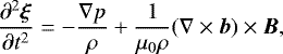
The plasma motion is described by the linear ideal MHD equations for an incompressible plasma: $$\nabla \cdot \xi =0,$$(2) $$\frac{{\partial }^2\xi }{\partial t^2}=-\frac{\nabla p}{\rho }+\frac{1}{{\mu }_0\rho }(\nabla \times b)\times B,$$(3) $$b=\nabla \times (\xi \times B).$$(4)

Here ξ is the plasma displacement, p the pressure perturbation, and b the magnetic field perturbation; B is the background magnetic field and μ₀ the magnetic permeability of free space. The vector B is parallel to the xy-plane. We have B =B₁ and ρ = ρ₁ for z < 0, and B =B₂ and ρ = ρ₂ for z > 0. In what follows we assume that ρ₁ < ρ₂.

Equations (2)–(4) have to be complemented with boundary conditions at z = 0. The first boundary condition is the kinematic condition: $${\xi }_{z1}={\xi }_{z2}=\eta ,$$(5)

where z = η(t, x, y) is the equation of perturbed interface, and the subscripts 1 and 2 indicate that a quantity is calculated for z < 0 and z > 0, respectively.The second boundary condition is the dynamic boundary condition. It states that the total pressure, plasma plus magnetic, has to be continuous at the discontinuity. In the linearised form it reads $$[[P-g\rho \eta ]]=0,$$(6)

where P = P +B ⋅b∕μ₀ is the perturbation of the total pressure (magnetic plus plasma) and the double brackets indicate the jump of a quantity across the discontinuity. To derive this boundary condition, we have used Eq. (1).

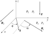Fig. 1 Sketch of the equilibrium. The gravity acceleration can change its own direction.

3 Derivation of the governing equation

In this section we derive the equation describing the dependence of the interface oscillation amplitude on time. We performed a Fourier analysis of the perturbations of all quantities with respect to x and y and take them proportional exp[i(k_xx + k_yy)]. Then Eqs. (2)–(4) reduce to $$\begin{array}{ll}\hfill & \frac{\text{d}{\xi }_z}{\text{d}z}+ik\cdot {\xi }_{\perp }=0,\hfill \\ \hfill & \rho \frac{{\text{d}}^2{\xi }_{\perp }}{\text{d}{t}^2}=-ikP+\frac{i}{{\mu }_0}{b}_{\perp }(k\cdot B),\hfill \\ \hfill & \rho \frac{{\text{d}}^2{\xi }_z}{\text{d}{t}^2}=-i\frac{\text{d}P}{\text{d}z}+\frac{i}{{\mu }_0}{b}_z(k\cdot B),\hfill \\ \hfill & b=i(k\cdot B)\xi ,\hfill \end{array}$$

where ξ_⊥ =ξ − ξ_ze_z, b_⊥ =b − b_ze_z, e_z is the unit vector in the z-direction, and k = (k_x, k_y, 0). Eliminating all variables in Eqs. (7)–(10) in favour of ξ_z and P, we obtain $$\begin{array}{ll}\hfill & \frac{{\text{d}}^{2}P}{\text{d}{z}^2}-k^{2}P=0,\hfill \\ \hfill & \frac{\text{d}P}{\text{d}z}=-\rho \frac{{\text{d}}^2{\xi }_z}{\text{d}{t}^2}-\frac{1}{{\mu }_0}{(k\cdot B)}^2{\xi }_z.\hfill \end{array}$$

The solution to Eq. (11) satisfying the condition that P → 0 as |z| →∞ is 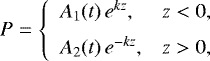$$P=\{\begin{array}{ll}{A}_1(t)e^{kz},\hfill & z<0,\hfill \\ A_2(t)e^{-kz},\hfill & z>0,\hfill \end{array}$$(13)

where A₁(t) and A₂ (t) are arbitrary functions. Taking Eq. (12) at z → −0 and z → +0, we obtain $$\begin{array}{l}k{A}_1(t)=-{\rho }_1\frac{{\text{d}}^2\eta }{\text{d}{t}^2}-\frac{1}{{\mu }_0}{(k\cdot B_1)}^2\eta ,\hfill \\ k{A}_2(t)={\rho }_2\frac{{\text{d}}^2\eta }{\text{d}{t}^2}+\frac{1}{{\mu }_0}{(k\cdot B_2)}^2\eta .\hfill \end{array}$$(14)

Substituting Eq. (13) into Eq. (6) yields $$A_1(t)-g{\rho }_1\eta =A_2(t)-g{\rho }_2\eta .$$(15)

Finally substituting Eq. (14) into Eq. (15), we obtain the Mathieu equation (Mathieu 1868) for η: $$\frac{{\text{d}}^2\eta }{\text{d}{t}^2}+[\frac{{(k\cdot B_1)}^2+{(k\cdot B_2)}^2}{{\mu }_0({\rho }_1+{\rho }_2)}-\frac{k{g}_0({\rho }_2-{\rho }_1)\cos (\Omega t)}{{\rho }_1+{\rho }_2}]\eta =0.$$(16)

4 Stability investigation

We use Eq. (16) to investigate the stability of the magnetic interface. We introduce the dimensionless quantities 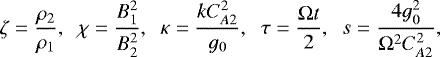$$\zeta =\frac{{\rho }_2}{{\rho }_1},\chi =\frac{B_1^2}{B_2^2},\kappa =\frac{k{C}_{A2}^2}{g_0},\tau =\frac{\Omega t}{2},s=\frac{4g_0^2}{{\Omega }^2{C}_{A2}^2},$$(17)

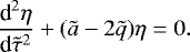
where $C_{A2}^2=B_2^2/{\mu }_0{\rho }_2$ is the Alfvén speed in the upper medium. We also introduce the angle α between B₁ and the x-axis, and the angle ϕ between k and the x-axis (see Fig. 1). Then we transform the Mathieu equation (Eq. (16)) to the canonical form: $$\frac{{\text{d}}^2\eta }{\text{d}{\tau }^2}+[a-2q\cos (2\tau )]\eta =0,$$(18)

where $$a=\frac{s\zeta {\kappa }^2[\chi {\cos }^2(\varphi -\alpha )+{\cos }^2\varphi ]}{\zeta +1},q=\frac{s\kappa (\zeta -1)}{2(\zeta +1)}.$$(19)

4.1 Constant gravity

For further reference, we recall the main results obtained by Ruderman et al. (2014) in the case of constant gravity. To obtain the constant gravity, we take Ω → 0. Since s →∞ as Ω → 0, we introduce new variables: $$\tilde{\tau }=\tau \sqrt{s},\tilde{a}=s^{-1}a,\tilde{q}=s^{-1}q.$$(20)

Then Eq. (18) reduces to $$\frac{{\text{d}}^2\eta }{\text{d}{\tilde{\tau }}^2}+(\tilde{a}-2\tilde{q})\eta =0.$$(21)

We look for the solution to this equation in the form of normal modes and take $\eta =e^{\sigma \tilde{\tau }}$. Then we obtain $${\sigma }^2=\frac{(\zeta -1)\kappa -\zeta {\kappa }^2[\chi {\cos }^2(\varphi -\alpha )+{\cos }^2\varphi ]}{\zeta +1}.$$(22)

It follows from this relation that there is an unstable normal mode (σ > 0) when κ < κ_c, where $${\kappa }_c=\frac{\zeta -1}{\zeta [\chi {\cos }^2(\varphi -\alpha )+{\cos }^2\varphi ]}.$$(23)

When $\kappa >{\overline{\kappa }}_c$ all perturbations are stable, where 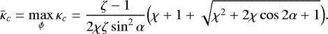$${\overline{\kappa }}_c={\displaystyle \underset{\varphi }{\text{max}}}{\kappa }_c=\frac{\zeta -1}{2\chi \zeta {\sin }^2\alpha }(\chi +1+\sqrt{{\chi }^2+2\chi \cos 2\alpha +1}).$$(24)

On the otherhand, all perturbations with κ satisfying $\kappa <{\widehat{\kappa }}_c$ are unstable, where 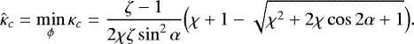$${\widehat{\kappa }}_c={\displaystyle \underset{\varphi }{\text{min}}}{\kappa }_c=\frac{\zeta -1}{2\chi \zeta {\sin }^2\alpha }(\chi +1-\sqrt{{\chi }^2+2\chi \cos 2\alpha +1}).$$(25)

When ϕ is fixed, the instability increment takes its maximum value σ_m(ϕ) at $\kappa =\frac{1}{2}{\kappa }_c$, where $${\sigma }_m(\varphi )={\displaystyle \underset{\kappa }{\text{max}}}\sigma =\frac{\zeta -1}{2\sqrt{\zeta (\zeta +1)[\chi {\cos }^2(\varphi -\alpha )+{\cos }^2\varphi ]}}.$$(26)

Finally, the maximum instability increment σ_M is given by 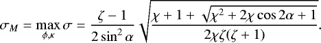$${\sigma }_M={\displaystyle \underset{\varphi ,\kappa }{\text{max}}}\sigma =\frac{\zeta -1}{2{\sin }^2\alpha }\sqrt{\frac{\chi +1+\sqrt{{\chi }^2+2\chi \cos 2\alpha +1}}{2\chi \zeta (\zeta +1)}}.$$(27)

This maximum is obtained when $\kappa =\frac{1}{2}{\kappa }_c$ and ϕ = ϕ_M, where 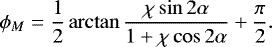$${\varphi }_M=\frac{1}{2}\arctan \frac{\chi \sin 2\alpha }{1+\chi \cos 2\alpha }+\frac{\pi }{2}.$$(28)

4.2 Oscillating gravity

We now proceed to studying stability in the presence of oscillating gravity. According to Floquet’s theorem (Floquet 1883; Abramowitz & Stegun 1964), Eq. (18) admits a solution η₊ (τ) = e^iλτF(τ), where F(τ) is a π-periodic function and λ is called the characteristic exponent. Since Eq. (18) is invariant under the substitution − τ → τ, it follows that η₋ (τ) = e^−iλτF(−τ) is also a solution. The functions η₊(τ) and η₋(τ) are linearly independent and the general solution to Eq. (18) is their linear combination unless λ is an integer number. Below we choose the solution with ℑ(λ) ≤ 0, where ℑ indicates the imaginary part of a quantity. When ℑ(λ) < 0, the instability increment is γ = −ℑ(λ). We note that an unstable mode amplitude does not grow exponentially as in the case when the equilibrium is stationary. Rather the perturbation amplitude increases e^πγ times after τ increases by π. In Fig. 2 the graphs of η₊(τ) are shown for a = 2 and a few values of q.

We consider a solution to Eq. (18) defined by the initial conditions: $${\eta }_1=1,\frac{\text{d}{\eta }_1}{\text{d}\tau }=0\text{\hspace{1em}at\hspace{1em}}\tau =0.$$(29)

The characteristic exponent is defined by the equation (Abramowitz & Stegun 1964) $$\cos (\pi \lambda )={\eta }_1(\pi ).$$(30)

In particular, it follows from this equation that λ is real when |η₁(π)|≤ 1, while it has a non-zero imaginary part when |η₁(π)| > 1. For fixed q, there is an infinite set {a_n}, n = 0, 1, 2, …, such that Eq. (18) has an even periodic solution with the period either π or 2π when a = a_n. There is also an infinite set {c_n}, n = 1, 2, …, such that Eq. (18) has an odd periodic solution with the period either π or 2π when a = c_n. As n →∞, a_n →∞ and c_n →∞. The quantities a_n and c_n are called the characteristic values of a. When a = a_n or a = c_n, the corresponding periodic solution has exactly n zeros in the interval τ ∈ [0, π). If q > 0, then the characteristic values are ordered as a₀ < b₁ < a₁ < b₂ < a₂ < ⋯. When q varies, a_n and c_n become functions of q; a_n (q) → n² and c_n (q) → n² as q → 0.

A very important property of Eq. (18) is that λ is real when a_n (q) ≤ a ≤ c_n+1(q), while it has a non-zero imaginary part when c_n(q) < a < a_n(q). Hence, a perturbation with a particular dimensionless wavenumber κ is unstable when c_n(q) < a < a_n(q) and stable otherwise. The curves a_n(q) and c_n(q) are shown in Fig. 3 for n = 1, 2, 3. The curve a₀(q) is not shown because a₀(q) < 0 for q > 0.

We have c₁(q₁) = 0 and a₁(q₂) = 0, where q₁ ≈ 0.925 and q₂ ≈ 7.514.

When κ varies whileall other parameters are fixed, we obtain a curve in the aq-plane parametrically defined by the equations a = a(κ) and q = q(κ). Eliminating κ from these equations, we obtain that this curve is a parabola, and its equation is $$a=K{q}^2,K=\frac{4\zeta (\zeta +1)[\chi {\cos }^2(\varphi -\alpha )+{\cos }^2\varphi ]}{s{(\zeta -1)}^2}.$$(31)

The parabola intersects the curve a_n(q) when q = q_an, while it intersects the curve c_n(q) when q = q_cn. The corresponding values of κ are κ = κ_an and κ = κ_cn. Then it follows that a perturbation is unstable if $\kappa \in {\displaystyle \underset{n=1}{\overset{\infty }{\cup }}({\kappa }_{\text{cn}},{\kappa }_{\text{an}})}$. When κ →∞, we have a →∞ and q →∞, while q∕a → 0. It is straightforward to see that in this case a_n(q) → n² and c_n(q) → n², which implies that q_an → nK^−1∕2 and q_cn → nK^−1∕2, and consequently $$\frac{{\kappa }_{\text{an}}}{n},\frac{{\kappa }_{\text{cn}}}{n}\to K^{-1/2}\frac{2(\zeta +1)}{s(\zeta -1)},\text{\hspace{1em}as\hspace{1em}}n\to \infty .$$(32)

It follows from this result that, in contrast to the case with constant gravity, for any N we can find such κ that κ > N and the perturbation with this dimensionless wavenumber is unstable. The dependences of q_an and q_cn on K are shown in Fig. 4.

In Fig. 5 the dependence of the instability increment γ = iλ on q is shown for various values of K. We can see that the gaps between the instability intervals are very small for small values of K, while they increase when K increases. We also calculated the maximum values of the instability increment γ with respect to q for q ∈ (q_cj, q_aj), j = 1, 2, 3. The dependences of these quantities on K are shown in Fig. 6. We notice that γ takes its absolute maximum in the interval (q_c2, q_a2) when K < K_int ≈ 0.181, and in the interval (q_c1, q_a1) when K > K_int.

We see that the maximum instability increment is a monotonically decreasing function of K. It is straightforward to show that K takes its minimum value with respect to ϕ at ϕ = ϕ_M, where ϕ_M is given by Eq. (28), and $$K_m={\displaystyle \underset{\varphi }{\text{min}}}K=\frac{4\zeta (\zeta +1)\left(\chi +1-\sqrt{{\chi }^2+2\chi \cos 2\alpha +1}\right)}{s{(\zeta -1)}^2}.$$(33)

After calculating K_m, we can determine the maximum instability increment γ_M using Fig. 6.

We now consider four limiting cases. First we assume that ρ₁ ≪ ρ₂, meaning ζ ≫1. In this case $$K_m\approx \frac{4}{s}\left(\chi +1-\sqrt{{\chi }^2+2\chi \cos 2\alpha +1}\right).$$(34)

Then we consider the case where B₁ ≪ B₂, so χ≪ 1. In this case $$K_m\approx \frac{8\chi \zeta (\zeta +1){\sin }^2\alpha }{s{(\zeta -1)}^2}.$$(35)

In the opposite case where B₁ ≫ B₂, we have χ ≫ 1. Then $$K_m\approx \frac{8\zeta (\zeta +1){\sin }^2\alpha }{s{(\zeta -1)}^2}.$$(36)

Finally, we study the case where the instability increment is much smaller than the gravity oscillation frequency. In the dimensionless variables, this condition reads γ ≪ 1. We are interested in the maximum growth rate rather than the growth rate of a particular mode. We can see in Fig. 5 that we can only have small maximum growth rate if K is large. We define the small parameter ϵ = K^−1∕2 ≪ 1. Figure 3 shows that a is close to n² on the parts of the dotted curve corresponding to unstable perturbations when K ≫ 1. We obtain a = n² taking q = nϵ, which implies that $q=O(ϵ)$. First we study the case with n = 1. Using the expansion valid for small q (Abramowitz & Stegun 1964), $$c_1(q)=1-q+O(q^2),a_1(q)=1+q+O(q^2),$$(37)

we obtain that the dotted curve in Fig. 3 intersects the curves a = c₁(q) and a = a₁(q) at q ≈ ϵ − ϵ²∕2 and q ≈ ϵ + ϵ²∕2, respectively. Then $q=ϵ+\overline{q}{ϵ}^2$ on the part of the dotted curve between the intersection points, where $\overline{q}$ is a free parameter. The equation of the dotted curve is now written as $a=1+2\overline{q}ϵ+{\overline{q}}^2{ϵ}^2$. Equation (18) is transformed to $$\frac{{\text{d}}^2\eta }{\text{d}{\tau }^2}+[1+2\overline{q}ϵ+{\overline{q}}^2{ϵ}^2-2(ϵ+\overline{q}{ϵ}^2)\cos (2\tau )]\eta =0.$$(38)

To calculate the increment for these values of $\overline{q}$, we need to find η₁(π), where η₁(τ) is the solution to Eq. (38) satisfying the initial conditions Eq. (29). To do this we use the regular perturbation method and put $${\eta }_1={\eta }_1^{(0)}+ϵ{\eta }_1^{(1)}+{ϵ}^2{\eta }_1^{(2)}+\cdots$$(39)

Substituting Eq. (39) in Eq. (38) and the boundary conditions Eq. (29), and collecting terms of the order of unity, we obtain $$\begin{array}{ll}\hfill & \frac{{\text{d}}^2{\eta }_1^{(0)}}{\text{d}{\tau }^2}+{\eta }_1^{(0)}=0,\hfill \\ \hfill & {\eta }_1^{(0)}=1,\frac{\text{d}{\eta }_1^{(0)}}{\text{d}\tau }=0\text{\hspace{1em}at\hspace{1em}}\tau =0.\hfill \end{array}$$

The solution to this initial value problem is $${\eta }_1^{(0)}=\cos \tau .$$(42)

Collecting the terms of the order of ϵ yields $$\begin{array}{ll}\hfill & \frac{{\text{d}}^2{\eta }_1^{(1)}}{\text{d}{\tau }^2}+{\eta }_1^{(1)}=2[\cos (2\tau )-\overline{q}]\cos \tau ,\hfill \\ \hfill & {\eta }_1^{(1)}=\frac{\text{d}{\eta }_1^{(1)}}{\text{d}\tau }=0\text{\hspace{1em}at\hspace{1em}}\tau =0.\hfill \end{array}$$

After straightforward calculation, we obtain $${\eta }_1^{(1)}=\frac{1-2\overline{q}}{2}\tau \sin \tau +\frac{1}{8}[\cos \tau -\cos (3\tau )].$$(45)

Collecting the terms of the order of ϵ², we obtain $$\begin{array}{ll}\hfill & \frac{{\text{d}}^2{\eta }_1^{(2)}}{\text{d}{\tau }^2}+{\eta }_1^{(2)}=2[\cos (2\tau )-\overline{q}]{\eta }_1^{(1)}+[2\overline{q}\cos (2\tau )-{\overline{q}}^2]\cos \tau ,\hfill \\ \hfill & {\eta }_1^{(2)}=\frac{\text{d}{\eta }_1^{(2)}}{\text{d}\tau }=0\text{\hspace{1em}at\hspace{1em}}\tau =0.\hfill \end{array}$$

The solution to this initial value problem is given by $$\begin{array}{l}{\eta }_1^{(2)}=\frac{1-4{\overline{q}}^2}{8}{\tau }^2\cos \tau +\frac{2\overline{q}-1}{16}\tau \sin (3\tau )+\frac{3\overline{q}-1}{8}\tau \sin \tau \\ +\frac{\cos (5\tau )}{192}-\frac{\overline{q}+1}{16}\cos (3\tau )+\frac{12\overline{q}+11}{192}\cos \tau .\end{array}$$(48)

Using Eqs. (39), (42), (45), and (48), we obtain $${\eta }_1(\pi )=-1+\frac{4{\overline{q}}^2-1}{8}{ϵ}^2{\pi }^2+\cdots$$(49)

Substituting this expression in Eq. (30) yields $$\cos (\pi \lambda )=-1+\frac{4{\overline{q}}^2-1}{8}{ϵ}^2{\pi }^2+O({ϵ}^3).$$(50)

When $\left|\overline{q}\right|\ge \frac{1}{2}$, the absolute value of the right-hand side of Eq. (50) does not exceed unity, λ is real, and the corresponding perturbation is neutrally stable. On the other hand, when $\left|\overline{q}\right|<\frac{1}{2}$, the absolute value of the right-hand side of Eq. (50) is larger than unity and λ is given by $$\lambda =1\pm \frac{iϵ}{2}\sqrt{1-4{\overline{q}}^2}+O({ϵ}^2).$$(51)

It follows from this result that $$\gamma =\frac{ϵ}{2}\sqrt{1-4{\overline{q}}^2},{\gamma }_m=\frac{ϵ}{2},$$(52)

where γ_m is the maximum value of the instability increment when the dotted curve is between the curves a = c₁(q) and a = a₁(q).

We nowconsider the part of the dashed curve in Fig. 3 that is in the sector bounded by the curves a = c_n(q) and a = a_n(q), n =2, 3, …. For q ≪1, we have $a_n=n^2+O(q^2)$ and $c_n=n^2+O(q^2)$ (Abramowitz & Stegun 1964). Since K = ϵ⁻², it follows that $q=nϵ(1+{ϵ}^2\overline{q})$ and $a=n^2(1+2{ϵ}^2\overline{q}+{ϵ}^4{\overline{q}}^2)$, where $\overline{q}$ is again a free parameter. Substituting these expressions in Eq. (18), we transform it to $$\frac{{\text{d}}^2\eta }{\text{d}{\tau }^2}+[n^2(1+2\overline{q}{ϵ}^2+{\overline{q}}^2{ϵ}^4)-2n(ϵ+\overline{q}{ϵ}^3)\cos (2\tau )]\eta =0.$$(53)

Then we again look for the solution to this equation satisfying the initial conditions Eq. (29) in the form of expansion: $${\eta }_1={\eta }_1^{(0)}+ϵ{\eta }_1^{(1)}+{ϵ}^2{\eta }_1^{(2)}+\cdots$$(54)

Substituting Eq. (54) in Eq. (53) and the boundary conditions Eq. (29) and collecting terms of the order of unity, we obtain $$\begin{array}{ll}\hfill & \frac{{\text{d}}^2{\eta }_1^{(0)}}{\text{d}{\tau }^2}+n^2{\eta }_1^{(0)}=0,\hfill \\ \hfill & {\eta }_1^{(0)}=1,\frac{\text{d}{\eta }_1^{(0)}}{\text{d}\tau }=0\text{\hspace{1em}at\hspace{1em}}\tau =0.\hfill \end{array}$$

The solution to this initial value problem is $${\eta }_1^{(0)}=\cos (n\tau ).$$(57)

Collecting the terms of the order of ϵ yields $$\begin{array}{ll}\hfill & \frac{{\text{d}}^2{\eta }_1^{(1)}}{\text{d}{\tau }^2}+n^2{\eta }_1^{(1)}=2n\cos (2\tau )\cos (n\tau ),\hfill \\ \hfill & {\eta }_1^{(1)}=\frac{\text{d}{\eta }_1^{(1)}}{\text{d}\tau }=0\text{\hspace{1em}at\hspace{1em}}\tau =0.\hfill \end{array}$$

After straightforward calculation, we obtain $${\eta }_1^{(1)}=\frac{1}{2}-\frac{1}{3}\cos (2\tau )-\frac{1}{6}\cos (4\tau )$$(60)

for n = 2, and $${\eta }_1^{(1)}=\frac{n}{4}\left(\frac{\cos [(n-2)\tau ]}{n-1}-\frac{\cos [(n+2)\tau ]}{n+1}-\frac{2n\cos (n\tau )}{n^2-1}\right)$$(61)

for n > 2. Collecting the terms of the order of ϵ yields $$\begin{array}{ll}\hfill & \frac{{\text{d}}^2{\eta }_1^{(2)}}{\text{d}{\tau }^2}+n^2{\eta }_1^{(2)}=2n{\eta }_1^{(1)}\cos (2\tau )-2\overline{q}\cos (n\tau ),\hfill \\ \hfill & {\eta }_1^{(2)}=\frac{\text{d}{\eta }_1^{(2)}}{\text{d}\tau }=0\text{\hspace{1em}at\hspace{1em}}\tau =0.\hfill \end{array}$$

After long but still straightforward calculation, we obtain that the solution to this initial value problem is given by $${\eta }_1^{(2)}=\left(\frac{5}{12}-\frac{\overline{q}}{2}\right)\tau \sin (2\tau )+\frac{\cos (6\tau )}{96}+\frac{\cos (4\tau )}{18}+\frac{29\cos (2\tau )}{288}-\frac{1}{6}$$(64)

for n = 2, and by $$\begin{array}{l}{\eta }_1^{(2)}=\left(\frac{1}{4(n^2-1)}-\frac{\overline{q}}{n}\right)\tau \sin (n\tau )+\frac{n\cos [(n+4)\tau ]}{32(n+1)(n+2)}\\ +\frac{n^2\cos [(n+2)\tau )}{8(n+1)(n^2-1)}-\frac{n(n^4-4n^3+n^2+16n-2)\cos (n\tau )}{16{(n^2-1)}^2(n^2-4)}\\ -\frac{n^2\cos [(n-2)\tau ]}{8(n-1)(n^2-1)}+\frac{n\cos [(n-4)\tau ]}{32(n-1)(n-2)}\end{array}$$(65)

for n > 2. It is easy to verify that ${\eta }_1^{(1)}(\pi )={\eta }_1^{(2)}(\pi )=0$. Then it follows from Eqs. (30), (54), and (57) that $$\cos (\pi \lambda )={(-1)}^n+O({ϵ}^3),$$(66)

which implies that $\gamma =O({ϵ}^{3/2})$. Hence, the increment in the area bounded by the curves a = c_n(q) and a = a_n(q) with n > 1 is much smaller than γ_m. Consequently, γ_m is the maximum value of the increment with respect to q when K = ϵ⁻².

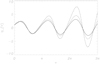Fig. 2 Dependence of η+ on τ for a = 2. The solud, dashed, and dash-dotted curves correspond to q = 1, 1.5, and 2, respectively.

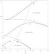Fig. 3 Stability diagram in the aq-plane. The solid and dashed lines show the curves an(q) and cn (q), respectively. The dotted line is the graph of the curve a = Kq2.

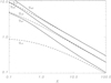Fig. 4 Dependences of qan and qcn on K for n = 1, 2, 3. The solid and dashed lines show the curves qan(K) and qcn (K), respectively.We note the logarithmic scale in the axes.

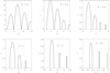Fig. 5 Dependences of the instability increment γ on q for various values of K.

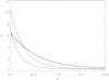Fig. 6 Dependences on K of the maximum with respect to q of the instability increment γ for q ∈ (qcj, qaj). The solid, dashed, and dash-dotted curves correspond to j = 1, 2, and 3, respectively. We note the logarithmic scale in the horizontal axis.

5 Application to the heliopause stability

We now apply the general results to the stability of a part of the heliopause near its apex point. The period of the gravity oscillation is equal to the solar cycle period, which is approximately 11 yr, and thus Ω ≈ 1.8 × 10⁻⁸ s⁻¹. Izmodenov et al. (2005, 2008) studied the effect of the solar cycle on the interaction of the solar wind with the interstellar medium. In particular, they found that the variation of the distance from the sun to the heliopause apex point oscillates with the amplitude about 2 AU about its mean value during the solar cycle. If we approximate this distance by d_mean − Acos(Ωt) with A = 2 AU, we obtain g₀ ≈ 9.7 × 10⁻⁵ m s⁻².

To estimate the magnetic field magnitude, we use the observational results obtained by Voyager 1 and reported by Burlaga & Ness (2014). The observed magnetic field was strongly fluctuating, but we can take as typical values B₁ = 0.2 nT and B₂ = 0.4 nT, where now the indices 1 and 2 refer to the inner and outer heliosheath, and thus χ =0.25. Burlaga et al. (2013) reported that the magnetic field direction changed by about 20° when Voyager 1 crossed the heliopause. Hence, we can take α = 20°.

We take the electron concentration in the interstellar medium equal to 4 × 10⁴ m⁻³ (e.g. Izmodenov 2009; Izmodenov & Alexashov 2015). The concentration of the neutral hydrogen is a few times higher. However, here we disregard the interaction between the changed and neutral components of the interstellar medium that occurs through the charge exchange. It is a very strong assumption which we will relax in the future study. Since the bow shock is weak (some authors even argue that it does not exist at all, e.g. McComas et al. 2012), we take the same value for the electron concentration at the heliopause. Then we obtain ρ₂ ≈ 6.7 × 10⁻²³ kg m⁻³. We also take the ratio of densities at the two sides of the heliopause equal to ζ = ρ₂∕ρ₁ = 50. Then we obtain C_A1 ≈ 154 km s⁻¹ and C_A2 ≈ 44 km s⁻¹, where C_A1 is the Alfvén speed below the interface. We also obtain s ≈ 0.062. Choosing the obtained values of the dimensionless parameters, we find K ≈ 3.17 and γ ≈ 0.5. The characteristic growth time of the instability is t_ins = 2∕(γΩ) ≈ 2.22 × 10⁸ s ≈ 7 years, which is comparable to the solar cycle period.

6 Summary and conclusions

We studied the magnetic Rayleigh–Taylor (MRT) instability of a magnetic interface in an infinitely conducting incompressible plasma in the presence of oscillating gravity acceleration. Our motivation was to study the stability of the heliopause in the vicinity of its apex point. During the solar cycle, the solar wind intensity varies. As a result, the heliopause moves back and forth, so the reference frame where it is at rest is non-inertial. The acceleration of this reference frame can be considered as an effective gravity.

In our investigation we assumed that the magnetic field has different directions at the two sides of the heliopause. We also used the approximation of incompressible plasma which enormously simplifies the analysis. The plasma in the heliosheath can hardly be considered as incompressible. The study of the compressibility effect of the MRT instability carried out by Ruderman (2017) showed that the compressibility can only substantially affect the MRT instability when the plasma beta is very small. This is definitely not the case in the heliosheath.

We derived the equation describing the temporal evolution of the interface shape and obtained that it is the Mathieu equation. When written in the dimensionless form it only contains two parameters, a and q. These two parameters are in turn functions of a few other dimensionless parameters: the density ratio ζ, the ratio of magnetic field magnitudes squared χ, the dimensionless wavenumber κ, and the parameter s proportional to the effective gravity acceleration amplitude squared. The parameter a, in addition, depends on two angles: the magnetic shear angle α and the angle between the perturbation wave vector and the magnetic field at one side of the interface ϕ. While the parameters ζ, χ, s, and α are related to the equilibrium state, κ and ϕ are the characteristic of a particular perturbation. Hence, they must be considered as free parameters.

The qa-plane is divided into an infinite number of interchanging stability and instability regions by curves a = c_n(q) and a = a_n(q). A particular perturbation is unstable if the point (q, a) is in the regions between the curves a = c_n(q) and a = a_n(q), while it is stable otherwise. Eliminating κ from the expressions for a and q in terms of the dimensionless parameter, we obtain that a = Kq², where K contains only one free parameter, ϕ. We studied the dependence of stability of perturbations on the parameters q and K. We showed that for any value of K > 0, there is an infinite sequence of intervals that do not overlap. A particular perturbation is unstable if q is in one of these intervals, and it is stable otherwise. We calculated the dependence of the increment on q for various values of K, and also the dependence on K of the maximum values of the increment when q is in the first three instability intervals. We found that all these values are monotonically decreasing functions of K. The maximum value of the increment in each instability interval depends on ϕ. The absolute maximum of the increment in each instability interval is taken when the function K(ϕ) takes its minimum.

We applied the general results to the heliopause stability. We found that the growth time of the fastest growing perturbation is about 7 yr. It is interesting to compare this result with that obtained under the assumption of constant gravity. If we assume that the heliopause is moving toward the interstellar medium with the maximum possible constant acceleration, which is g₀, then, using Eq. (27) we obtain that the instability growth time is approximately 1.5 yr, almost five times less than that found in the model with the oscillating gravity.

In closing we would like to say, as was shown by Borovikov et al. (2008), that charge exchange can cause the heliopause RT instability even when its position does not change. This implies that to get mode realistic modes describing the heliopause MRT instability we must include the effect of charge exchange. However, this is a problem for future studies.

Acknowledgements

The author acknowledges the financial support of STFC.

References

All Figures

	Fig. 1 Sketch of the equilibrium. The gravity acceleration can change its own direction.
In the text

	Fig. 2 Dependence of η+ on τ for a = 2. The solud, dashed, and dash-dotted curves correspond to q = 1, 1.5, and 2, respectively.
In the text

	Fig. 3 Stability diagram in the aq-plane. The solid and dashed lines show the curves an(q) and cn (q), respectively. The dotted line is the graph of the curve a = Kq2.
In the text

	Fig. 4 Dependences of qan and qcn on K for n = 1, 2, 3. The solid and dashed lines show the curves qan(K) and qcn (K), respectively.We note the logarithmic scale in the axes.
In the text

	Fig. 5 Dependences of the instability increment γ on q for various values of K.
In the text

	Fig. 6 Dependences on K of the maximum with respect to q of the instability increment γ for q ∈ (qcj, qaj). The solid, dashed, and dash-dotted curves correspond to j = 1, 2, and 3, respectively. We note the logarithmic scale in the horizontal axis.
In the text

References

- Abramowitz, M., & Stegun, I. 1964, Handbook of Mathematical Functions, National Bureau of Standards Applied Mathematics Series − 5 (Washington, DC: U.S. Government Printing Office) [Google Scholar]
- Baranov, V. B. 2009a, Space Sci. Rev., 143, 449 [NASA ADS] [CrossRef] [Google Scholar]
- Baranov, V. B. 2009b, Space Sci. Rev., 142, 23 [NASA ADS] [CrossRef] [Google Scholar]
- Baranov, V. B., Krasnobaev, K. V., & Kulikovskii, A. G. 1971, Sov. Phys. Dokl., 15, 791 [NASA ADS] [Google Scholar]
- Baranov, V. B., Fahr, H. J., & Ruderman, M. S. 1992, A&A, 261, 341 [NASA ADS] [Google Scholar]
- Borovikov, S. N., Pogorelov, N. V., Zank, G. P., & Kryukov, I. A. 2008, ApJ, 682, 1404 [NASA ADS] [CrossRef] [Google Scholar]
- Bucciantini, N., Amato, E., Bandiera, R., Blondin, J. M., & Del Zanna L. 2004, A&A, 423, 253 [NASA ADS] [CrossRef] [EDP Sciences] [Google Scholar]
- Burlaga, L. F., & Ness, N. F. 2014, ApJ, 784, 146 [NASA ADS] [CrossRef] [Google Scholar]
- Burlaga, L. F., Ness, N. F., & Stone, E. C. 2013, Science, 341, 147 [NASA ADS] [CrossRef] [Google Scholar]
- Carlyle, J., & Hillier, A. 2017, A&A, 605, A101 [NASA ADS] [CrossRef] [EDP Sciences] [Google Scholar]
- Chalov, C. V. 1994, Planet. Space Sci., 42, 55 [NASA ADS] [CrossRef] [Google Scholar]
- Díaz, A. J., Soler, R., & Ballester, J. L. 2012, ApJ, 754, 41 [NASA ADS] [CrossRef] [Google Scholar]
- Díaz, A. J., Khomenko, E., & Collados, M. 2014, A&A, 564, A97 [NASA ADS] [CrossRef] [EDP Sciences] [Google Scholar]
- Fahr, H. J., Neutsch, W., Grzedzielski, S., Macek, W., & Ratkiewicz-Landowska, R. 1986, Space Sci. Rev., 43, 329 [NASA ADS] [CrossRef] [Google Scholar]
- Floquet, G. 1883, Ann. Ecole Norm. Sup., 12, 47 [CrossRef] [Google Scholar]
- Florinski, V., Zank, G. P., & Pogorelov, N. V. 2005, J. Geophys. Res., 110, A07104 [NASA ADS] [CrossRef] [Google Scholar]
- Hillier, A., Isobe, H., Shibata, K., & Berger, T. 2011, ApJ, 736, L1 [NASA ADS] [CrossRef] [Google Scholar]
- Hillier, A., Berger, T., Isobe, H., & Shibata, K. 2012a, ApJ, 746, 120 [NASA ADS] [CrossRef] [Google Scholar]
- Hillier, A., Isobe, H., Shibata, K., & Berger, T. 2012b, ApJ, 756, 110 [NASA ADS] [CrossRef] [Google Scholar]
- Isobe, H., Miyagoshi, T., Shibata, K., & Yokoyama, T. 2005, Nature, 434, 478 [NASA ADS] [CrossRef] [Google Scholar]
- Isobe, H., Miyagoshi, T., Shibata, K., & Yokoyama, T. 2006, PASJ, 58, 423 [Google Scholar]
- Izmodenov, V. 2009, Space Sci. Rev., 143, 139 [NASA ADS] [CrossRef] [Google Scholar]
- Izmodenov, V., & Alexashov, D. B. 2015, ApJS, 220, 32 [NASA ADS] [CrossRef] [Google Scholar]
- Izmodenov, V., Malama, Y., & Ruderman, M. S. 2005, A&A, 429, 1069 [NASA ADS] [CrossRef] [EDP Sciences] [Google Scholar]
- Izmodenov, V., Malama, Y., & Ruderman, M. S. 2008, Adv. Space Res., 41, 318 [NASA ADS] [CrossRef] [Google Scholar]
- Jun, B.-I., Norman, M. L., & Stone, J. M. 1995, ApJ, 453, 332 [NASA ADS] [CrossRef] [Google Scholar]
- Liewer, P. C., Karmesin, S. R., & Brackbill, J. U. 1996, J. Geophys. Res., 101, 17119 [NASA ADS] [CrossRef] [Google Scholar]
- Mathieu, E. 1868, J. Math. Pures Appl., 137 [Google Scholar]
- McComas, D. J., Alexashov, D., Bzowski, M., et al. 2012, Science, 336, 1291 [NASA ADS] [CrossRef] [Google Scholar]
- Pogorelov, N. V., Fichtner, H., Czechowski, A., et al. 2017a, Space Sci. Rev., 212, 193 [NASA ADS] [CrossRef] [Google Scholar]
- Pogorelov, N. V., Heerikhuisen, J., Roytershteyn, V., et al. 2017b, ApJ, 845, 9 [NASA ADS] [CrossRef] [Google Scholar]
- Ruderman, M. S. 2015, A&A, 580, A37 [NASA ADS] [CrossRef] [EDP Sciences] [Google Scholar]
- Ruderman, M. S. 2017, Sol. Phys., 292, 47 [NASA ADS] [CrossRef] [Google Scholar]
- Ruderman, M. S., & Fahr, H. J. 1993, A&A, 275, 635 [NASA ADS] [Google Scholar]
- Ruderman, M. S., & Fahr, H. J. 1995, A&A, 299, 258 [NASA ADS] [Google Scholar]
- Ruderman, M. S., & Belov, N. A. 2010, J. Phys. Conf. Ser., 216, 012016 [NASA ADS] [CrossRef] [Google Scholar]
- Ruderman, M. S., Terradas, J., & Ballester, J. L. 2014, ApJ, 785, A110 [NASA ADS] [CrossRef] [Google Scholar]
- Ruderman, M. S., Ballai, I., Collados, M., & Khomenko, E. 2017, A&A, 609, A23 [Google Scholar]
- Ryutova, M. P., Berger, T., Frank, Z., Tarbell, T., & Title, A. 2010, Sol. Phys., 267, 75 [Google Scholar]
- Stone, J. M., & Gardiner, T. 2007, ApJ, 671, 1696 [Google Scholar]
- Taroyan, Y., & Ruderman, M. S. 2011, Space Sci. Rev., 158, 505 [NASA ADS] [CrossRef] [Google Scholar]
- Terradas, J., Oliver, R., & Ballester, J. L. 2012, A&A, 541, A102 [NASA ADS] [CrossRef] [EDP Sciences] [Google Scholar]