| Issue |
A&A
Volume 615, July 2018
|
|
|---|---|---|
| Article Number | A145 | |
| Number of page(s) | 5 | |
| Section | Planets and planetary systems | |
| DOI | https://doi.org/10.1051/0004-6361/201731941 | |
| Published online | 30 July 2018 | |
A search for transiting planets in the β Pictoris system★
1
Leiden Observatory, Leiden University,
PO Box 9513,
2300
RA
Leiden, The Netherlands
e-mail: This email address is being protected from spambots. You need JavaScript enabled to view it.
2
Institut für Astro- und Teilchenphysik, Universität Innsbruck,
Technikerstrasse 25,
6020
Innsbruck, Austria
3
Graz University of Technology, Institute of Communication Networks and Satellite Communications,
Infeldgasse 12,
8010
Graz, Austria
Received:
13
September
2017
Accepted:
22
March
2018
Abstract
Context. Transiting exoplanets provide an opportunity for the characterization of their atmospheres, and finding the brightest star in the sky with a transiting planet enables high signal-to-noise ratio observations. The Kepler satellite has detected over 365 multiple transiting exoplanet systems, a large fraction of which have nearly coplanar orbits. If one planet is seen to transit the star, then it is likely that other planets in the system will transit the star too. The bright (V = 3.86) star β Pictoris is a nearby young star with a debris disk and gas giant exoplanet, β Pictoris b, in a multi-decade orbit around it. Both the planet’s orbit and disk are almost edge-on to our line of sight.
Aims. We carry out a search for any transiting planets in the β Pictoris system with orbits of less than 30 days that are coplanar with the planet β Pictoris b.
Methods. We search for a planetary transit using data from the BRITE-Constellation nanosatellite BRITE-Heweliusz, analyzing the photometry using the Box-Fitting Least Squares Algorithm (BLS). The sensitivity of the method is verified by injection of artificial planetary transit signals using the Bad-Ass Transit Model cAlculatioN (BATMAN) code.
Results. No planet was found in the BRITE-Constellation data set. We rule out planets larger than 0.6 RJ for periods of less than 5 days, larger than 0.75 RJ for periods of less than 10 days, and larger than 1.05 RJ for periods of less than 20 days.
Key words: planets and satellites: detection / planets and satellites: individual: β Pic / techniques: photometric
Based on data collected by the BRITE-Constellation satellite mission built, launched, and operated thanks to support from the Austrian Aeronautics and Space Agency and the University of Vienna, the Canadian Space Agency (CSA), and the Foundation for Polish Science & Technology (FNiTP MNiSW) and National Centre for Science (NCN).
Elise Richter Fellow of the Austrian Science Funds (FWF).
© ESO 2018
1 Introduction
The discovery of the first extrasolar planets over twenty years ago through the radial velocity technique (Mayor & Queloz 1995; Marcy & Butler 1995) rapidly led to the detection of multiple planet systems (Butler et al. 1999; Fischer et al. 2002; Marcy et al. 2001). As the number of exoplanet detections reached into the hundreds, the architecture of these systems began to show a wide range of diversity in both their semimajor axis distribution and their eccentricities. The unexpected detection of giant planets with semimajor axes smaller than the orbit of Mercury in our own solar system rapidly led to the first detection of a transiting planet (Charbonneau et al. 2000; Brown et al. 2001) and the subsequent characterization of its atmosphere (Charbonneau et al. 2002). The Kepler satellite led to the discovery of over 2000 exoplanets, along with over 365 multiple-planet systems where the mutual inclinations of the planets is in the range of 1 to 2 degrees (Fabrycky et al. 2014).
The signal-to-noise ratio of a transiting planet is partly driven by the apparent brightness of the host star, and so several searches are underway to find the brightest star in the sky with a transiting planet. Several transit searches therefore focus on the brightest stars, including the Multi-site All-Sky CAmeRA (MASCARA), which surveys the sky from the ground for stars with magnitudes from 4 to 8 (Talens et al. 2017), and the Kilodegree Extremely Little Telescope (KELT), which searches for transits from the ground for magnitudes from 8 to 10 (Pepper et al. 2007). There are also future projects for measuring transits around bright stars via space telescopes. The Transiting Exoplanet Survey Satellite (TESS) is planned for launch in mid-2018 and will look at stars 10–100 times as bright as Kepler (Ricker et al. 2014). Further in the future is the PLAnetary Transits and Oscillations of stars (PLATO). Planned for launch in 2024 it will, among other things, look for terrestrial planets around stars similar to our Sun1. Looking for the brightest star with a transiting Earth-like planet is of great importance, as this would make it an ideal target for further investigation with a telescope such as the James Webb Space Telescope. The present-day interest in Earth-like exoplanets is confirmedby the attention that the TRAPPIST-1 planetary system received following its discovery in 2017 (Gillon et al. 2017).
The β Pictoris system is a young (~23 Myr; Mamajek & Bell 2014) and nearby (19.3 pc; van Leeuwen 2007) system, which consists of the star, a debris disk with several kinematical components, and one gas giant planet (β Pictoris b). The star is known to be a δ Scuti pulsator: three pulsation frequencies were discovered by Koen (2003) using ground-based photometric time series. Shortly after that, Koen et al. (2003) reported the presence of 14 pulsation frequencies found from dedicated spectroscopic time series.
In 1983, IRAS detected excess infrared material around β Pictoris (Aumann 1985). A year later, a circumstellar disk was observed optically around the star by Smith & Terrile (1984). The disk is nearly edge-on and its outer extent varies from 1450 to 1835 AU (Larwood & Kalas 2001). Distinct belts around β Pictoris have been detected at distances of 14, 28, 52, and 82 AU (Wahhaj et al. 2003), kinematically suggesting the presence of planets in the system. The inner disk of β Pictoris is warped, implying the presence of a secondary companion inside the disk (Mouillet et al. 1997). The stellar and planetary parameters for β Pictoris andits planet are listed in Table 1.
A planet was directly imaged in 2009 (Lagrange et al. 2009, 2010) at a wavelength of 3.5 μm by the NACO camera on the VLT at Paranal. The planet β Pictoris b will not transit its host star because of its distance from the star and its inclination of 88.81°± 0.12° as seen from Earth (Wang et al. 2016); see Fig. 1. Planets form from a natal circumstellar disk, and therefore are coplanar with coaligned orbital angular momentum vectors, as seen in multiple transiting systems in Kepler and the solar system (Fabrycky et al. 2014). The high inclination of β Pictoris and the morphology of the disk suggests that if there are any other planets in the β Pictoris system then they will also have high inclinations and possibly transit the stellar disk.
We examine photometric data from the BRITE-Constellation nanosatellite mission, which observed β Pictoris for δ Scuti pulsations in 2015. In Sect. 2 we describe the BRITE data set, and Sect. 3 is dedicated to the analysis we use on this data. The results and conclusions are discussed in Sect. 4 and 5.
Stellar and planetary parameters for β Pictoris.
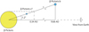 |
Fig. 1 Imageof the β Pictoris system showing the geometry of β Pictoris b and a coplanar third planet interior to b. A planet coplanar with β Pictoris b i = 88.81° will transit along diminishing chords of the star out to a radius of 0.34 au, corresponding to an orbital period of 54 d. |
2 Data
2.1 BRITE-Constellation
The data for this study was obtained using BRITE-Heweliusz (BHr), one of the BRIght Target Explorer (BRITE)-Constellation nanosatellites. BRITE-Constellation (Weiss et al. 2014; Pablo et al. 2016; Popowicz 2016) is a fleet of nanosatellites (6 launched; 5 operational) operated by a consortium consisting of Austria, Canada, and Poland). BHr carries a red filter (Weiss et al. 2014), and has a nearly circular Sun-synchronous orbit with an altitude of approximately 635 km and a period of 97.1 minutes.
2.2 β Pictoris data
Observations were made between 2015 March 16 UT and 2015 June 02 UT for a total of 78 days. The original data set, which can be retrieved from the BRITE Public Data Archive,2 consists of 47 330 individual photometric measurements obtained in stare mode (Popowicz et al. 2017). After main data reduction pipeline processing (Popowicz et al. 2017), the light curve was decorrelated using the steps described in Pigulski et al. (2016) and points with excessive photometric deviations and noise were removed. The final data set contains 44 246 measurements (see Fig. 2).
The frequency analysis of the BRITE photometric time series was performed using the software package Period04 (Lenz & Breger 2005), which combines Fourier and least-squares algorithms. Frequencies were then pre-whitened and considered to be significant it their amplitudes exceeded 4× the local noise level in the amplitude spectrum (Breger et al. 1993; Kuschnig et al. 1997). We identified eight δ Scuti pulsation frequencies in the range between 32 and 61 d−1 with amplitudes between 0.3 and 1.4 m mag, which were then subtracted from the data. The residual light curve was normalized to unity and yields a standard deviation of 0.86%. A detailed discussion of the pulsational content of β Pictoris is summarized in Zwintz (2017) and will be described fully together with a detailed asteroseismic interpretation in Zwintz et al. (in prep).
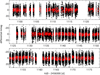 |
Fig. 2 Light curve of the detrended photometry from the BRITE satellite for β Pictoris over the 78-day run. The original detrended data are shown in black, data binned over three-minute intervals are shown in red. Each subset covers a time span of 27 days. |
3 Analysis and results
We use the Box-Fitting Least Squares (BLS) algorithm to perform a search for transiting planets in the BRITE data. BLS is an algorithm (designed by Kovács et al. 2002) that analyzes a photometric time series and searches for a flat bottomed planetary transit, returning the most probable orbital periods and transit depth. For this study, the “eebls” routine3 was used. These are Python bindings for the original Fortran implementation of BLS from Kovács et al. (2002), modified for edge effects when the transit event happens to be divided between the first and last bins, as the original BLS yielded lower detection efficiency in these cases.
We first determined the parameters using an artificial data set with the same cadence and noise properties as the BRITE data set. Transits were injected into this artificial data and the rate of recovery was determined from many random trials.
3.1 Determining the BLS parameters
A number of parameters can be set for the eebls routine: 1) nf, the numberof frequency points in which the spectrum is computed; 2) fmin ∕fmax, the minimum/maximum frequency; 3) df, the frequency step size; 4) nb, the number of bins in the folded time series at any test period; 5) qmi∕qma, the minimum/maximum fractional transit length to be tested. The values of these parameters used in this study can be seen in Table 2.
A value of 1000 and 16 000 was used for nf for the majority of the simulations. The minimum frequency fmin was chosen as 1∕Pmax, the maximum period to test for, and in the same way fmax = 1∕Pmin. The value ofdf was calculated from the nf and fmin (and fmax) values usingthe following formula:
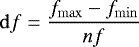 (1)
(1)
The value for nb is 1750, which allows for 25 data points per bin for the longest trial period. For qmi and qma we used the following equation to obtain transit durations:
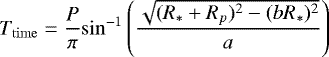 (2)
(2)
with
 (3)
(3)
where P is the period of the planet and b the impact parameter. A planet orbiting β Pictoris will have a transit duration of 7.5 h for a 30-day period, corresponding to a transit fraction of about 0.01, dropping to a transit period of 2.4 h for a one-day orbital period, corresponding to a transit fraction of 0.1. To make sure the values of qmi and qma covered the period range of this search, they were set to qmi = 0.005 and qma = 0.12.
Parameter values in the eebls routine.
3.2 Sensitivity plots
To test the sensitivity of the BLS algorithm in recovering transits from the BRITE data, fake transits were inserted into the data set and then recovered. These transits were simulated with the Python package BATMAN (Bad-Ass Transit Model cAlculatioN; Kreidberg 2015). With BATMAN we simulate the transit curve given a planet radius Rp (i) and periods P(i), along with the stellar mass and radius and the orbital inclination (listed in Table 1). A nonlinear limb darkening model was used.
3.2.1 White noise
The time data points and standard deviation of the flux from the BRITE data were used to generate a data set similar to the BRITE data with Gaussian noise. The BATMAN curves were inserted into this generated data set and the BLS algorithm applied to generate a periodogram. The highest peak in the periodogram was given a rank k = 0, the second highest peak k = 1, the third highest peak k = 2, and so on. If the period Pk=0 was within 5% of the inserted period P(i) (so that  ), it was considered a successful retrieval. For each trial of P and R, a new transit model was injected into the data with the transit time T randomized over the interval 0 to P. The rank of the period peak that corresponds to the injected orbital period P was noted. The mean rank
  was calculated as
 (4)
(4)
where  means that the correct period was identified in all the trials.
The success rate of this retrieval told us whether or not we would be able to find planets with radius Rp (i) and period P(i) in the BRITE data. The period was varied between 1 and 30 days in steps of 0.25 days. The 30-day upper limit was set to ensure three transits detectable within the 78-day window.
The model radius was varied between 0.15 and 1.5 RJ in steps of 0.15 RJ. The upper limit for this radius was based on the Lagrange et al. (2013) radial velocity-based detection limits, where they found that for a period of 3 days a planet of 1.5 MJ can remain undetected with the current available data, while for a period of 10 days this is 2.1 MJ. The results are displayed in a sensitivity map of period P and radius R (see Fig. 3).
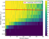 |
Fig. 3 Sensitivity map for β Pictoris using simulated Gaussian noise. The red line indicates the detection limit set by Lagrange et al. (2013). |
3.2.2 δ Scuti pulsation analysis
The orbital period of the satellite (97.1 min) imposes a periodic window function on the photometry, and this appears as spectral power at 0.067469 days. The δ Scuti pulsations from the star alias with this window function and act as a source of systematic error in the photometry. This is seen in the reduced sensitivity of the BLS analysis carried out on the β Pictoris photometric data seen in Fig. 4.
The δ Scuti pulsations are removed according to the prescription in Zwintz (2017). The subtraction of the pulsations results in a decrease in power across the periodogram, as seen in Fig. 5. The amplitudes of several peaks are seen to decrease and several drop below the mean noise floor of the data. The transit injection analysis is repeated for this data set. A visual inspection of the period folded light curves for the ten highest ranked periods was made. No plausible transiting candidate is present in the data. To determine the upper limits of the sensitivity of this analysis, a sensitivity map of this data is made to determine which combinations of period and radius can be excluded. The result is shown in Fig. 6.
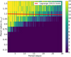 |
Fig. 4 Sensitivity map for the β Pictoris photometry. The red line indicates the detection limit from Lagrange et al. (2013). |
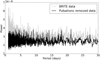 |
Fig. 5 Periodogram of the original and the pulsation removed BRITE data. |
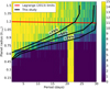 |
Fig. 6 Sensitivity map for β Pictoris using the pulsation removed data set. The red line indicates the detection limit set by Lagrange et al. (2013), whereas the solid black lines are an indication of the limits set by this study. |
4 Discussion
A radial velocity study by Lagrange et al. (2013) constrained possible massive companions to β Pictoris, placing upper limits on the mass of any companions. To evaluate the currently existing limits, we converted the mass limits into limits for the radii. We used the Python package called Forecaster4 by Chen & Kipping (2017). For a given mass, younger planets have a larger radii at younger ages as they have a greater effective temperature. This package is calibrated for much older planets, and it defines a conservative lower limit on the mass. This package takes as input the mean and standard deviation of the mass and returns a mean and standard deviation of the radius. Using this package, the limits for the mass given in Lagrange et al. (2013) were converted into limits for the radius. The values we calculated are shown in Table 3. The limits from Lagrange et al. (2013) are shown as a red line in all the figures. Comparing these values with the sensitivity map of the original BRITE data, seen in Fig. 4 we show a significant increase in sensitivity for smaller orbital periods.
Mass-radius relationship derived for Lagrange et al. (2013).
5 Conclusions
The sensitivity map of the pulsation removed BRITE data lowers the limits of possible exoplanets as set by Lagrange et al. (2013). As was discussed in Table 3, the limits set by that study were 1.2 RJ for 3 days, 1.18 RJ for 10 days, and 1.15 RJ for 100 days. We find limits of 0.6 RJ for 5 days, 0.75 RJ for 10 days, and1.0 RJ for 20 days. However, because of the degeneracies in converting radii to masses, these limits are best kept as constraints on the radius of a possible β Pictoris c.
With β Pictoris b moving through inferior conjunction in 2017 (Wang et al. 2016), several projects are conducting photometricand spectroscopic monitoring campaigns looking for the signatures of circumplanetary material in the Hill sphere. In order to provide a good baseline for this transit, BRITE-Constellation has revisited β Pictoris from November 4, 2016, to June 22, 20175. The corresponding data are currently being reduced. A photometric monitoring project called bRing (Stuik et al. 2017) has two cameras surveying β Pictoris in South Africa and Australia. The camera in South Africa already started observing in February2017, and the one based in Australia started observing in November 2017 6,7.
Although such observations are intended for detecting the β Pictoris b Hill sphere, they can also be used as additional data for the method used in this study. By doubling or tripling the number of data points, the sensitivity of the plot to smaller radii planets will increase and enable tighter constraints on, or the detection of, smaller planets.
Acknowledgements
Based on data collected by the BRITE-Constellation satellite mission, designed, built, launched, operated, and supported by the Austrian Research Promotion Agency (FFG), the University of Vienna, the Technical University of Graz, the Canadian Space Agency (CSA), the University of Toronto Institute for Aerospace Studies (UTIAS), the Foundation for Polish Science & Technology (FNiTP MNiSW), and the National Science Centre (NCN). This research made use of Astropy, a community-developed core Python package for Astronomy (Astropy Collaboration 2013). KZ acknowledges support by the Austrian Fonds zur Förderung der wissenschaftlichen Forschung (FWF, project V431-NBL).
References
- Astropy Collaboration, Robitaille, T. P., Tollerud, E. J. et al. 2013, A&A, 558, A33 [NASA ADS] [CrossRef] [EDP Sciences] [Google Scholar]
- Aumann, H. H. 1985, PASP, 97, 885 [NASA ADS] [CrossRef] [Google Scholar]
- Breger, M., Stich, J., Garrido, R., et al. 1993, A&A, 271, 482 [NASA ADS] [Google Scholar]
- Brown, T. M., Charbonneau, D., Gilliland, R. L., Noyes, R. W., & Burrows, A. 2001, ApJ, 552, 699 [NASA ADS] [CrossRef] [Google Scholar]
- Butler, R. P., Marcy, G. W., Fischer, D. A., et al. 1999, ApJ, 526, 916 [NASA ADS] [CrossRef] [Google Scholar]
- Charbonneau, D., Brown, T. M., Latham, D. W., & Mayor, M. 2000, ApJ, 529, L45 [NASA ADS] [CrossRef] [PubMed] [Google Scholar]
- Charbonneau, D., Brown, T. M., Noyes, R. W., & Gilliland, R. L. 2002, ApJ, 568, 377 [NASA ADS] [CrossRef] [Google Scholar]
- Chen, J., & Kipping, D. 2017, ApJ, 834, 17 [Google Scholar]
- Chilcote, J., Pueyo, L., De Rosa, R. J., et al. 2017, AJ, 153, 182 [NASA ADS] [CrossRef] [Google Scholar]
- Fabrycky, D. C., Lissauer, J. J., Ragozzine, D., et al. 2014, ApJ, 790, 146 [NASA ADS] [CrossRef] [Google Scholar]
- Fischer, D. A., Marcy, G. W., Butler, R. P., Laughlin, G., & Vogt, S. S. 2002, ApJ, 564, 1028 [NASA ADS] [CrossRef] [Google Scholar]
- Gillon, M., Triaud, A. H. M. J., Demory, B.-O., et al. 2017, Nature, 542, 456 [NASA ADS] [CrossRef] [PubMed] [Google Scholar]
- Koen, C. 2003, MNRAS, 341, 1385 [NASA ADS] [CrossRef] [Google Scholar]
- Koen, C., Balona, L. A., Khadaroo, K., et al. 2003, MNRAS, 344, 1250 [NASA ADS] [CrossRef] [Google Scholar]
- Kovács, G., Zucker, S., & Mazeh, T. 2002, A&A, 391, 369 [NASA ADS] [CrossRef] [EDP Sciences] [Google Scholar]
- Kreidberg, L. 2015, PASP, 127, 1161 [NASA ADS] [CrossRef] [Google Scholar]
- Kuschnig, R., Weiss, W. W., Gruber, R., Bely, P. Y., & Jenkner, H. 1997, A&A, 328, 544 [NASA ADS] [Google Scholar]
- Lagrange, A.-M., Gratadour, D., Chauvin, G., et al. 2009, A&A, 493, L21 [NASA ADS] [CrossRef] [EDP Sciences] [Google Scholar]
- Lagrange, A.-M., Bonnefoy, M., Chauvin, G., et al. 2010, Science, 329, 57 [NASA ADS] [CrossRef] [PubMed] [Google Scholar]
- Lagrange, A.-M., Meunier, N., Chauvin, G., et al. 2013, A&A, 559, A83 [NASA ADS] [CrossRef] [EDP Sciences] [Google Scholar]
- Larwood, J. D., & Kalas, P. G. 2001, MNRAS, 323, 402 [NASA ADS] [CrossRef] [Google Scholar]
- Lenz, P., & Breger, M. 2005, Communications in Asteroseismology, 146, 53 [Google Scholar]
- Mamajek, E. E., & Bell, C. P. M. 2014, MNRAS, 445, 2169 [NASA ADS] [CrossRef] [Google Scholar]
- Marcy, G. W., & Butler, R. P. 1995, BAAS, 27, 1379 [NASA ADS] [Google Scholar]
- Marcy, G. W., Butler, R. P., Fischer, D., et al. 2001, ApJ, 556, 296 [NASA ADS] [CrossRef] [Google Scholar]
- Mayor, M., & Queloz, D. 1995, Nature, 378, 355 [NASA ADS] [CrossRef] [Google Scholar]
- Mouillet, D., Larwood, J. D., Papaloizou, J. C. B., & Lagrange, A. M. 1997, MNRAS, 292, 896 [NASA ADS] [CrossRef] [PubMed] [Google Scholar]
- Pablo, H., Whittaker, G. N., Popowicz, A., et al. 2016, PASP, 128, 125001 [NASA ADS] [CrossRef] [Google Scholar]
- Pepper, J., Pogge, R. W., DePoy, D. L., et al. 2007, PASP, 119, 923 [NASA ADS] [CrossRef] [Google Scholar]
- Pigulski, A., Cugier, H., Popowicz, A., et al. 2016, A&A, 588, A55 [NASA ADS] [CrossRef] [EDP Sciences] [Google Scholar]
- Popowicz, A. 2016, in Space Telescopes and Instrumentation 2016: Optical, Infrared, and Millimeter Wave, Proc. SPIE, 9904, 99041R [NASA ADS] [CrossRef] [Google Scholar]
- Popowicz, A., Pigulski, A., Bernacki, K., et al. 2017, A&A, 605, A26 [NASA ADS] [CrossRef] [EDP Sciences] [Google Scholar]
- Ricker, G. R., Winn, J. N., Vanderspek, R., et al. 2014, in Space Telescopes and Instrumentation 2014: Optical, Infrared, and Millimeter Wave, Proc. SPIE, 9143, 914320 [Google Scholar]
- Smith, B. A., & Terrile, R. J. 1984, Science, 226, 1421 [NASA ADS] [CrossRef] [PubMed] [Google Scholar]
- Stuik, R., Bailey, J. I., Dorval, P., et al. 2017, A&A, 607, A45 [NASA ADS] [CrossRef] [EDP Sciences] [Google Scholar]
- Talens, G. J. J., Spronck, J. F. P., Lesage, A.-L., et al. 2017, A&A, 601, A11 [NASA ADS] [CrossRef] [EDP Sciences] [Google Scholar]
- van Leeuwen F., 2007, Hipparcos, the New Reduction of the Raw Data, Astrophys. Space Sci. Lib., 350 [CrossRef] [Google Scholar]
- Wahhaj, Z., Koerner, D. W., Ressler, M. E., et al. 2003, ApJ, 584, L27 [NASA ADS] [CrossRef] [Google Scholar]
- Wang, J. J., Graham, J. R., Pueyo, L., et al. 2016, AJ, 152, 97 [NASA ADS] [CrossRef] [Google Scholar]
- Weiss, W. W., Rucinski, S. M., Moffat, A. F. J., et al. 2014, PASP, 126, 573 [NASA ADS] [CrossRef] [Google Scholar]
- Zwintz, K. 2017, Proc. third BRITE-Constellation Sci. Conf., in press, [arXiv:1712.03496] [Google Scholar]
All Tables
All Figures
|
Fig. 1 Imageof the β Pictoris system showing the geometry of β Pictoris b and a coplanar third planet interior to b. A planet coplanar with β Pictoris b i = 88.81° will transit along diminishing chords of the star out to a radius of 0.34 au, corresponding to an orbital period of 54 d. |
| In the text | |
|
Fig. 2 Light curve of the detrended photometry from the BRITE satellite for β Pictoris over the 78-day run. The original detrended data are shown in black, data binned over three-minute intervals are shown in red. Each subset covers a time span of 27 days. |
| In the text | |
|
Fig. 3 Sensitivity map for β Pictoris using simulated Gaussian noise. The red line indicates the detection limit set by Lagrange et al. (2013). |
| In the text | |
|
Fig. 4 Sensitivity map for the β Pictoris photometry. The red line indicates the detection limit from Lagrange et al. (2013). |
| In the text | |
|
Fig. 5 Periodogram of the original and the pulsation removed BRITE data. |
| In the text | |
|
Fig. 6 Sensitivity map for β Pictoris using the pulsation removed data set. The red line indicates the detection limit set by Lagrange et al. (2013), whereas the solid black lines are an indication of the limits set by this study. |
| In the text | |
Current usage metrics show cumulative count of Article Views (full-text article views including HTML views, PDF and ePub downloads, according to the available data) and Abstracts Views on Vision4Press platform.
Data correspond to usage on the plateform after 2015. The current usage metrics is available 48-96 hours after online publication and is updated daily on week days.
Initial download of the metrics may take a while.