| Issue |
A&A
Volume 615, July 2018
|
|
|---|---|---|
| Article Number | A39 | |
| Number of page(s) | 8 | |
| Section | Planets and planetary systems | |
| DOI | https://doi.org/10.1051/0004-6361/201731775 | |
| Published online | 09 July 2018 | |
Interior structure models and fluid Love numbers of exoplanets in the super-Earth regime★
Institute of Physics, University of Rostock,
18051
Rostock,
Germany
e-mail: This email address is being protected from spambots. You need JavaScript enabled to view it.
Received:
15
August
2017
Accepted:
8
February
2018
Abstract
Space missions such as CoRoT and Kepler have made the transit method the most successful technique in observing extrasolar planets. However, although the mean density of a planet can be derived from its measured mass and radius, no details about its interior structure, such as the density profile, can be inferred so far. If determined precisely enough, the shape of the transiting light curve might, in principle, reveal the shape of the planet, and in particular, its deviation from spherical symmetry. These deformations are caused, for instance, by the tidal interactions of the planet with the host star and by other planets that might orbit in the planetary system. The deformations depend on the interior structure of the planet and its composition and can be parameterized as Love numbers kn. This means that the diversity of possible interior models for extrasolar planets might be confined by measuring this quantity. We present results of a wide-ranging parameter study in planet mass, surface temperature, and layer mass fractions on such models for super-Earths and their corresponding Love numbers. Based on these data, we find that k2 is most useful in assessing the ratio of rocky material to iron and in ruling out certain compositional configurations for measured mass and radius values, such as a prominent core consisting of rocky material. Furthermore, we apply the procedure to exoplanets K2-3b and c and predict that K2-3c probably has a thick outer water layer.
Key words: equation of state / planets and satellites: terrestrial planets / planets and satellites: composition / planets and satellites: individual: K2-3 system / planets and satellites: interiors / planet–star interactions
Tables of the computed k2 coefficients are only available at the CDS via anonymous ftp to cdsarc.u-strasbg.fr (130.79.128.5) or via http://cdsarc.u-strasbg.fr/viz-bin/qcat?J/A+A/615/A39
© ESO 2018
1 Introduction
The current statistics of detected extrasolar planets implies that the main fraction is represented by super-Earths and mini-Neptunes, that is, by planets in the mass range 1–10 ME (Rauer et al. 2014). Understanding their formation, interior structure, and evolution constitutes a major challenge to planetary physics since the number of observational constraints is small and their accuracy is, in general, poor compared to the planets in the solar system. However, super-Earths offer a much broader parameter space for mass M, radius R, composition, and the thermophysical properties of planetary materials. Any progress in describing super-Earths will simultaneously allow us to test models applied to the rocky planets in the solar system, in particular, Earth.
Studies on the interior of super-Earths typically start from our knowledge on the structure of Earth, which is summarized in the Preliminary Reference Earth Model (PREM; Dziewonski & Anderson 1981). For instance, mass-radius relations for super-Earths have recently been calculated based on the PREM by Zeng et al. (2016). Since Earth-like planets have to be characterized, it is necessary to check the degree to which models predicted for super-Earths reproduce the Earth’s structure so that the conclusions drawn on their interior and evolution are well founded (Unterborn et al. 2016). However, the equation-of-state (EOS) data for the major constituents and the temperature- and pressure-dependent transport and thermal properties such as viscosity, thermal conductivity, thermal expansivity, and heat capacity are not well-known for large parts of the parameter region that is relevant for their interior (Stamenkovic et al. 2012; Valencia et al. 2009). Therefore, simple scaling laws have been applied for these quantities in order to give predictions for the rheology of super-Earths and to derive possible interior structures and evolution scenarios (see Stamenkovic et al. 2011; Wagner et al. 2011; Duffy et al. 2015). Alternatively, a grid of models for exoplanets has been calculated mainly based on extrapolated EOS data for the main constituents inside these planets and assuming that they are differentiated, that is, that layered structure models can be applied (Zeng & Sasselov 2013).
The limited number of observational constraints compared to solar system planets is the bottleneck for a better understanding of extrasolar planets. If the radial-velocity (RV) technique can be applied to known transiting planets or transit timing variations (TTV) are observed, at least the mass and radius of the planet are known. Still, Valencia et al. (2013) showed that even though radius measurements can constrain the H/He content in the atmosphere of a super-Earth, its information about the water-to-rock ratio in the bulk material is limited.
With over 4000 planets and planet candidates discovered, the Kepler mission makes the transit method the most successful detection method so far (Coughlin et al. 2016; Morton et al. 2016). In addition to progress in observational techniques such as atmospheric spectroscopy (see, e.g., Seager & Deming 2010), the determination of additional parameters that describe the gravitational field of extrasolar planets is highly desirable. If such parameters could be derived, valuable information on the interior composition and the differentiation processes in the planet would be gained.
In the context of the importance for the habitability of a planet, differentiation may be second only to the existence of liquid water. Distinct fluid layers of electrically conducting materials such as liquid iron or superionic water are needed to drive the generation of a planetary dynamo. Without the resulting magnetic field, stellar winds (streams of charged particles) would be able to carry away the planet atmosphere and leave potential life on the surface vulnerable to ionizing UVradiation from the parent star. Tian & Stanley (2013) found that low-mass planets up to about 5 ME tend to develop more axial-dipolar dominated magnetic fields, similar to the magnetic field of Earth. Compared to this, heavier planets promote magnetic fields with more pronounced higher-order multipole moments. However, this can depend strongly on the age and stellar irradiation of the planet. As Zeng & Sasselov (2014) showed, an isolated H2O-rich super-Earth (or one that does not receive much irradiation from its host star) tends to be mostly solid after an age of about 3 Gyr, thus losing its ability to maintain a magnetic field.
More than 100 years ago, Love (1911) introduced the numbers hn and kn, which characterize the gravity field of a planet. If these Love numbers were known for extrasolar planets, we could infer details of their gravity field and therefore of their internal density distribution. Measuring the Love number is therefore a promising method for considerably reducing the number of possible interior models for extrasolar planets and to make an important step toward a better understanding of their formation and evolution processes. For tidal interactions between two celestial bodies (e.g., a planet and its host star), the Love number hn describes the resulting radial displacement of a point on the planet surface. On the other hand, the quantity kn describes the variation in gravity potential that is due to the interactions. Shida (1912) later added a third set ln that quantifies tangential displacement.
In the case of a fully fluid body, an assumption that we make in the current work, we obtain h2 = k2 + 1 for the lowest order. Because of this simple relation and because the lowest order would be the easiest to measure, we only calculate k2. Furthermore, with Love numbers, we refer to kn in particular.
So far, Love number calculations have mostly been applied to solar system planets and moons as well as to extrasolar ice giants and hot Jupiters (see, e.g., Kramm et al. 2011, 2012; Sohl et al. 2003; Ragozzine & Wolf 2009). Nettelmann et al. (2011) investigated the structure and thermal evolution of GJ 1214b. Their preferred model for this planet has large amounts of water mixed into a hydrogen–helium envelope and is therefore comparable to Uranus and Neptune. Batygin et al. (2009), Mardling (2007), and Becker & Batygin (2013) explored the internal structure of a transiting exoplanet by examining the orbital interaction with a second planet. In these systems the apses of the two planets are aligned, and their precession is mostly driven by the transiting planet’s gravitational distortions.
The upcoming PLATO 2.0 mission (Rauer et al. 2014) benefits from the enormous recent development in exoplanet science. One of the central goals is to measure the radius and the mass of extrasolar planets with so far unprecedented accuracy, in particular, for super-Earths and mini-Neptunes in the mass range 1–10 ME. Furthermore, it is expected that the changes of the transit light curve during ingress and egress that are due to a non-spherical planet shape can be measured by PLATO 2.0 over several transit events. The deformation of an exoplanet with 2 RE, for example, and an Earth-like flattening on a ten-day orbit around a Sun-like star is just above the detectability threshold for an inclination of 90° (Csizmadia, priv. comm.). If the inclination is lower, the change in the light curve is expected to be even more pronounced. Such observations would directly provide the Love number k2, which is a measure for the density profile throughout the planet and a further constraint for the diversity of possible interior models.
The approach we use to calculate the Love number based on a density profile has previously been outlined by Kramm et al. (2011). They reported on a degeneracy of k2 for planetary models assuming three layers for the interior structure. For two-layer profiles, they find a monotonically decreasing behavior of the Love number. However, they used an analytical polytropic model for their calculations. Here, we improve the method by using EOSs that stem from density functional theory molecular dynamics (DFT-MD) simulations, for instance. Our calculations show that degeneracy can occur for two-layer models as well. For planets with two solid layers, it is most prominent for masses similar to that of Earth. If the outermost layer is water, the effect extends to even higher masses, and for a hydrogen–helium mixture, it does not occur at all for planets with masses below ten Earth masses.
We here expand our knowledge of possible interior compositions of extrasolar planets. With these data and a broader planet range from ongoing satellite missions, evolutionary models can be calculated more precisely. This would in turn lead to a better understanding of the history of our own solar system.
We start our paper by briefly outlining the calculation of structure models and the Love numbers (Sect. 2). In Sect. 3 we present the results of a more general parameter study for the interior of extrasolar planets and their Love numbers. Based on these results, we also make predictions for the extrasolar planets K2-3b and c. We conclude the paper in Sect. 4 and offer an outlook on future research.
2 Method
2.1 Structure models
Transitions between layers often occur gradually in planets. To reduce numerical effort, we neglected compositional gradients and used three-layer models instead to approximate two solid inner layers (Fe and MgO) and an outer volatile layer (H2, He, and H2O), or a solid core and two volatile layers, respectively. Our models were calculated based on the numerical integration of the two structural differential equations:

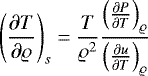
They describe the hydrostatic equilibrium and mass conservation, respectively. The procedure starts at the planet surface where the mass coordinate m equals the input parameter of the total mass M. The outer boundary conditions are the surface pressure PS = 1 bar and the surface temperature TS. The surface density follows from the EOS as ϱS = ϱ(PS, TS). For the total radius R = r(M), a first value is guessed, and with this, the gravitational acceleration can be calculated as g0 = GM∕R2, with the gravitational constant G.
When the integration reaches m = 0 or r ≤ 0, the calculation is stopped. With m and r of the last integration step, it is determined whether the model can be regarded as having converged or if the total radius needs to be adjusted. This iterative process is repeated until the inner boundary condition r(m = 0) = 0 is fulfilled. For numerical convergence we use the criterion |r(m = 0)|≤ 1 m. The centralvalues of physical quantities are denoted with the index c.
Other input parameters for the computer code are the mass fractions of the distinct layers Mi with i = 1⋯3, counting from the center. For the purpose of this work, these mass fractions are treated as non-dimensional, which means that they need to add up to unity ∑ Mi = 1. From the integration coordinate m, the corresponding EOS can be selected.
2.2 Equations of state
The solid layers are modeled with a generalized Rydberg EOS for iron as described by Wagner et al. (2011) or with rocky material, forwhich we use a revised version of the magnesium oxide EOS, first published by Cebulla & Redmer (2014). In this, we include both B1 and B2 phases. As volatile materials we use water (see Wagner & Pruß 2002), hydrogen, and helium, as described by Becker et al. (2014), and a mixture of the latter two of solar composition, which we refer to as (H2/He)sol.
Because of the nature of our three-layer models, we neglect material mixture at layer boundaries. In general, such behavior would homogenize the density distribution and should lead to a slight increase in the corresponding Love number (see next section).
Iron and magnesium oxide layers are typically characterized by high pressures. Hence we treat them as solid. For such phases, the pressuredependency of the density profile is far more important than the temperature dependency, which is shown in Table 1. There, we calculated one-layer models with 300 K or 2500 K surface temperature for MgO and (H2/He)sol. For isothermal solid magnesium oxide, the differences in the resulting radii are on the order of a few percent. However, for an isothermal solar composition, the radius increases tenfold. We therefore made the approximation of treating the iron and rocky layers as isothermal.
As for volatiles the temperature dependency of the density cannot be neglected, we assume a fully convective layer and use an isentropic temperature profile. Starting from the entropy total differential, the equation
 (3)
(3)
can be derived. Here u denotes the internal energy per unit mass.
The isentrope of the outermost layer is determined by surface temperature and pressure alone and can therefore becalculated before the main integration; this is the same throughout all iterations. In the case of a second inner adiabatic layer, the corresponding isentrope changes with every iteration, depending on the thermodynamic conditions at its upper boundary. To obtain a mixture EOS of hydrogen and helium, we apply the ansatz of linear mixing as described by DeMarcus (1958) and Peebles (1964). For a given pressure P and temperatureT, the density and internal energy are given by

Here, ϱH/He and uH/He are the values for the pure elements. Y and X = 1 − Y denote the mass fractions of helium and hydrogen, respectively. For the solar composition, we have Y = 0.2485 (see, Eddy 1979) and therefore set X = 0.7515.
Effect of surface temperature and type of temperature profile on a planet radius and Love number for models with one layer.
2.3 Fluid Love number
The fluid Love number describes the response of the internal mass distribution of a planet to a gravitational perturbance, for example, by the host star or a satellite. The external potential can be described using Legendre polynomials Pn (see, e.g., Zharkov & Trubitsyn 1978)
 (6)
(6)
where M⋆ is the perturbing mass and a its distance to the planet. The radial coordinate s describes some point within the planet, and θ is the angle between this coordinate and the axis that connects the centers of the two celestial bodies. The induced potential of the planet can be expressed as

where Kn is the so-called Love function of degree n, and its corresponding value at the surface s = R is referred to as the Love number kn.
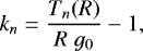
To calculate kn, we adopted the procedure developed by Zharkov & Trubitsyn (1978). The Love number can then be expressed by
 (9)
(9)
where g0 is the surface gravity of the unperturbedplanet, and the function Tn is required to fulfill the differential equation
![Mathematical equation: \begin{eqnarray*} T_n''(s) + \frac{2}{s} T_n'(s) + \left[ \frac{4\pi G \varrho'(s)}{V'(s)} - \frac{n(n+1)}{s^2} \right] T_n(s) = 0. \end{eqnarray*}](/articles/aa/full_html/2018/07/aa31775-17/aa31775-17-eq7.png) (10)
(10)
To integrate this equation, we need the density distribution ϱ and the potential of the unperturbed planet V, as well as their first derivatives with respect to s (primed quantities).
To ensure that Tn is a continuous function over the whole profile, the inner boundary conditions:
![Mathematical equation: \begin{eqnarray}T_n(b^+) &=& T_n(b^-),\\ T_n'(b^+) &=& T_n'(b^-) + \frac{4\pi G}{V'(b)}\left[\varrho(b^-)-\varrho(b^+)\right]T_n(b), \end{eqnarray}](/articles/aa/full_html/2018/07/aa31775-17/aa31775-17-eq8.png)
have to be fulfilled at an internal density jump at s = b. In these equations, b− and b+ denote the inner and outer side of the density jump, respectively.
In the work presented here we are interested in first-order deviations from spherical symmetry. The possible values of k2 lie in the range from 0 to 1.5, where the upper margin corresponds to a homogeneous density. As more mass is concentrated within the center, the Love number decreases, possibly by several orders of magnitude.
Similarly to the gravitational moments J2n, the Love numbers depend on the density profile of the planet. The important difference is that while the first set of quantities is susceptible to the mass distribution in the outer layers (Nettelmann et al. 2012), the second set is governed by the mass distribution near the center. We therefore have additional planetary quantities at our disposal to characterize a planet and benchmark our models.
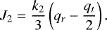
Heller et al. (2011) showed that the obliquity of a short-period planet decreases over times of mostly less 109 years (they call this time the tilt erosion time). After this time, the rotation axis is perpendicular to the orbital plane, and with that, also to the tidal deformation. In such cases, J2 can be calculated to first order from the Love number (Love 1911)
 (13)
(13)
Here qr and qt are dimensionless quantities that set gravitational acceleration in comparison to that of rotational and tidal potentials, respectively. With ν the angular spin frequency of the planet and M⋆ the host star mass, these constants are
 (14)
(14)
2.4 Planets
For our parameter study we fixed the surface pressure to PS = 1 bar and varied the planet mass (M = 1⋯10 ME), surface temperature (TS = 300⋯2500 K), and the composition of the three layers, and for a fixed set of these quantities, we also varied the mass fractions of the different layers (M3 = 10−7⋯100, M2 = 10−2⋯100, M1 = 1 − M2 − M3).
In addition, we also present results on the inner two planets of the system K2-3. Table 2 lists mass, radius, mean density, and surface temperature of these planets. K2-3b with its 8.4 ME and mean density of 5.16 g cm−3 lies between the mass-radius curves of ice-rich and silicate-rich planets (see for comparison Fig. 4 in Rauer et al. 2014). K2-3c, on the other hand, with only one quarter of that mass and about half the mean density, is very close to the curve of ice-rich planets. Although the mass error boundaries are listed, we limited our calculations to the mean value.
Parameters for the star K2-3 and its two planets K2-3b and c.
3 Results
We start by comparing results obtained with our procedure with the Love number of Earth. According to Lambeck (1980), we have k2, Earth = 0.934. We used anisothermal two-layer model of 300 K with a mass fraction of the iron core of M1 = 0.32 (Stacey & Davis 2008) and a MgO mantle. Our procedure yields R = 1.004 RE and k2 = 0.8999. This discrepancy of about 4% in the Love number can be attributed to the use of magnesium oxide as solid mantlematerial. Most of the Earth mantle consists of the silicate perovskite called bridgmanite (MgSiO3, Tschauner et al. 2014) mixed with ferrous rocky materials. This composition has a slightly higher density than MgO. Therefore the (Mg,Fe)SiO3 mantle is thinner, the core mass is less highly concentrated in the center (compared to the total radius), and thus k2 increases.
A silicate perovskite EOS might reproduce the Love number of Earth better than the magnesium oxide EOS. However, we used MgO because the DFT-MD data set provided for the relevant pressure and temperature range is extensive. Available EOS data for MgSiO3, on the otherhand, are commonly based on Vinet and Birch-Murnaghan fits to a limited amount of experimental or ab initio data (see, e.g., Sakai et al. 2016).
In the following, we first present the results of our parameter study and explain for which cases the Love number can be useful to constrain models. In the second part we apply our procedure to the planets K2-3b and c.
3.1 Parameter study
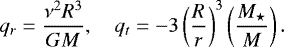
In the following section, a combination of parameters is denoted in parentheses. For example (Fe MgO (H2/He)sol, 3 ME, 500 K) corresponds to all models ofmass 3 ME with an iron core, a magnesium oxide lower mantle, an upper mantle of solar composition, and a surface temperature of 500 K. This example for the parameter study is shown in Fig. 1. In the left panel, the color plot shows the radius a model has for a specific set of parameters. We neglected all models with a mass fraction of the iron core higher than 0.9. Models at the right edge of the plot, that is, those with volatile mass fractions close to one, would result in radii of several ten Earth radii, which we can exclude according to the current statistics of extrasolar planets.
The right plot shows the resulting Love numbers and the possible range, which stretches over more than three orders of magnitude. k2 along a constant M2 very clearly shows the degeneracy for models with more than two layers. This effect can also be seen along constant M3, although not as pronounced in logarithmic scale. This difference stems from the density difference, which is much larger between a solid and a volatile material than between two solids. Close to the upper left and the two lower corners, the Love number comes closest to the value for an homogeneous density as the planetary structure is mainly governed by only one of the three layers.
The black solid iso-radius lines in Fig. 1 mark models with the same radius. To determine how the Love number k2 can be useful to constrain models, we examined our results along these lines. The first characteristic property we are interested in is the mass ratio of rocky mantle to iron core material. For the simplification that the cores of Earth and Mercury consist of pure iron and their mantles of pure MgO, their respective Fe/MgO mass ratios are 0.484 and 2.125 (Stacey & Davis 2008). In Fig. 2, this mass ratio of models along the iso-radius lines of Fig. 1 is plotted as a function of k2. For a constant radius, the Love number does not appear to span more than one order of magnitude. However, the corresponding Fe/MgO fractions can change by a factor of 1000. As the lowest iso-radius line has the highest Love numbers, a measurement of k2 can be especially useful for low-radius super-Earths to narrow down their Fe/MgO ratio.
The effect of surface temperature TS and planet mass M on the behaviorof k2 is shown in Fig. 3. In the upper panel we set the mass constant to 3 ME and varied the surface temperature from 300 K to 2500 K. All plotted lines are iso-radius lines for two Earth radii. Especially in the upper mantle, a higher temperature leads to a more strongly diluted material. Therefore this layer must have a lower mass fraction than at colder temperatures to meet the radius condition. As the curves cover the same range of k2 for all temperatures, the Love number cannot be used to gain information on the surface temperature. However, if the temperature is determined with a suitable assumption, such as radiative equilibrium with the host star, k2 may help in constrainingthe mass fraction of the uppermost layer. This appears to work best for colder planets as the slope of the iso-radius line in the k2 –M3 diagram is smaller compared to higher TS. From the radius R and M3, it is then possible to derive M1 and M2 as well.
The lower panel of Fig. 3 shows the dependency of k2 on the planet mass. This quantity was varied from 1 ME to 10 ME, while the surface temperature was kept constant at 1000 K. For higher masses, the slope of the curves decreases strongly. This leads to a narrower range of k2 values covered. However, the range of the upper layer mass fraction increases by several orders of magnitude. As an exoplanet mass is determined via the RV method, the Love number is not very useful to constrain this quantity. Nevertheless, when RV is combined with a measurement of k2, it is again possible to constrain the sizes of the inner layers.
So far, we specifically considered models with twice the radius of Earth. As a next step, we present k2 as a function of the planet radius in Fig. 4. Larger radii obviously allow for larger mass fractions of the volatile material. Asthe radius increases, the Love number decreases by several orders of magnitude. This can be explained by recalling that the mass fractions of the solid materials are still much larger than that of the upper mantle, but their layer radii do not increase much. The concentration of mass in the planet center therefore increases strongly.
At higher masses, the outer volatile layer is more compressed by gravitational pull. The mass is therefore less highly concentrated in the center, which again increases k2. Similarly to a mass measurement via RV, a radius measurement via transit photometry in conjunction with a k2 measurement could be used to narrow down the different mass fractions.
Finally, Fig. 5 shows the influence of the composition of the three layers. No models with 2 RE were found for a total of three parameter combinations. In the case of (Fe MgO H2O, 3 ME, 300 K), thedensity of water is too high compared to hydrogen and helium, for instance. Even a planet made of pure water with this mass and surface temperature would have a radius of only around 1.93 RE.
The comparison of models with a water and a (H2/He)sol layer shows the effect of core material on the resulting Love numbers. A first observation is that a decrease in density in the core increases the minimum possible k2 value. This is expected as a lower density leads to a decrease in mass concentration in the center. However, the maximum possible k2 value increases in such a way that the Love number range in a logarithmic representation is much narrower for the lower-density core material. For higher surface temperatures or masses, it may happen that no models (for the given radius) can be found at all. For example, for models with 3 ME, 300 K, and 2 RE (upper plot in Fig. 5), the possible range of k2 values becomes narrower for magnesium oxide cores compared to iron cores. If the surface temperature is increased to 2500 K, the behavior is similar: there is a narrow range for models with iron cores, while no models at all can be found for magnesium oxide cores. Analogous findings can be made when TS is kept at 1000 K and the mass is set to 1 ME and 10 ME (lower plot in Fig. 5). Owing to this decreased range of k2 for more extreme conditions, the Love number can be used to distinguish between different core materials and narrow down the chemical composition of the innermost layer.
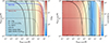 |
Fig. 1 Example results of the parameter study for a planet with 3 ME, TS = 500 K, iron core, MgO lower mantle, and a H/He mixture for the upper mantle of solar composition. The two axes depict the mass fractions of the mantle layers, and the color code represents the resulting radius (left) and Love number k2 (right). For the further evaluation of the results, we neglect models with an iron core mass fraction of 0.9 or higher (models below the thin dotted line). The black solid lines are iso-radius lines for models with 1.5, 2, 3, or 4 Earth radii. Models withan Earth-like (mercury-like) Fe/MgO mass ratio lie along the blue (brown) line. |
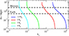 |
Fig. 2 Fe/MgO mass ratio as a function of k2 for the four iso-radius lines from Fig. 1. The corresponding ratios of Earth and Mercury are indicated by the two horizontal lines. |
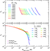 |
Fig. 3 Influence of surface temperature (upper panel) and planet mass (lower panel) on the Love number k2 of objects with R = 2 RE. All models have an iron core, a MgO lower mantle, and a (H2/He)sol upper mantle. The magenta (violet) crosses mark the intersections of the iso-radius lines with the line corresponding to Earth-like (Mercury-like) Fe/MgO mass ratio. The curves for 3 ME and surface temperatures of 300 K, 500 K, and 2500 K are longer because they were created with higher resolution in M2 and M3 (for Figs. 1 and 4) and therefore reach slightly higher values for M2. |
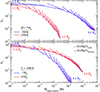 |
Fig. 4 Love number k2 as a functionof upper mantle mass fraction for different temperatures (top), planet masses (bottom), and planet radii. The iso-radius lines range from 1.0 RE (where applicable) to 4.4 RE, with a step width of 0.2 RE. The composition is the same as in Fig. 3. Here we show results for the lowest and highest temperatures and masses, respectively. |
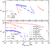 |
Fig. 5 Influence of the chemical composition of the three layers (different line styles). Masses and surface temperatures are the same as in Fig. 4, while all lines depict the two-Earth-radii iso-radius lines. No models were found for the parameter combinations (Fe MgO H2 O, 3 ME, 300 K) (MgO H2O (H2/He)sol, 3 ME, 2500 K), and (MgO H2O (H2/He)sol, 10 ME, 1000 K). |
3.2 K2-3b and c
For our models for the planets of the K2-3 system, we always took the mean value of mass and examined the upper and lower boundaries for the radius. When we were unable to find models for one of these radii, we used the mean value instead.
Figure 6 compares our results for the two planets K2-3b and c. When we consider models for K2-3b with an outer water mantle, the possible mass fractions for this layer range from about 0.1% up to 46%, andthe Love number ranges from 0.94 down to 0.33. In the case of a hydrogen–helium envelope, k2 can even decrease down to 0.11. However, as this material is much more diluted, the possible mass fractions drop to a maximum of 0.4%. For these two compositions, the iso-radius lines end before reaching M3 = 10−7, our lower bound. Models with two volatile layers are possible even at lower M3, although the Love number does not change much. It has a much smaller range than for the other two compositions, ranging only from 0.12 to 0.37 for iron cores and from 0.55 to 0.61 for magnesium oxide cores. This behavior was described before for the curve with 10 ME and 1000 K in Fig. 5. The models with an MgO core allow only for mass fractions of the upper mantle of up to M3 = 6 × 10⁻⁷. The water mass fraction of the respective curve ranges from 10% to 20%.
Comparing these results to those of K2-3c, we find that the latter results all lie above our lower M3 boundary. Furthermore, the models with a lower magnesium oxide mantle cover a considerably smaller range for the Love number k2. As described previously, K2-3c is expected to bear much more water than K2-3b. According to our assumptions, models with a water-rich outer layer would have at least 44% and up to 74% H2 O by mass (see the inset in Fig. 6). For this composition, k2 ranges from 0.81 to 0.62. Such a small range for this composition is reminiscent of small and cold planets from our parameter study (see Fig. 5).
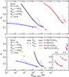 |
Fig. 6 Results for the two exoplanets K2-3b and K2-3c. When possible, we show iso-radius curves for the upper and lower radius boundaries. In contrast to all previous figures, the Love number here is a linear axis. |
4 Conclusion
We have calculated three-layer models for exoplanets in the super-Earth regime (1–10 ME) and their corresponding Love numbers k2. This quantity describes the central mass concentration within the planet interior and becomes degenerate even for two-layer models. Nevertheless, if combined with measurements of other planetary properties, it can be used to confine models for given exoplanets.
The most promising application is in constraining the mass ratio of iron to rock material in the interior of low-radius objects (see Fig. 2). Furthermore, the strength of a known Love number lies not in determining the materials that can be found in a planet, but rather in ruling out certain configurations. In the case of models with an iron core, a lower water mantle, and an upper mantle composed of a hydrogen–helium mixture, the resulting range of k2 is especially narrow for hot or high-mass planets (see Fig. 5). If this thin range is not included in some measurement for the Love number, a lower water mantle would not be possible for such planets.
In addition to the parameter study, we also presented results for two planets that where discovered by the K2 mission. In particular, we find that K2-3c data on mass and radius support models with up to 74% water by mass and a k2 of around 0.7.
While the current data on exoplanet Love numbers are limited to a few cases, a new evaluation of several years of Kepler transit light curves may provide us with k2 values for some more planets. This would allow us to improve the method of inferring structure models from k2 even more before first data from PLATO 2.0 are even available.
Acknowledgments
We thank Daniel Cebulla for providing the MgO data and Nadine Nettelmann, Frank Wagner, Frank Sohl, and Szilard Csizmadia for helpful discussions. Furthermore, we thank Szilard Csizmadia for his calculations of the Love number measurability. We warmly thank the anonymous referee for providing helpful comments to improve the possible effect of this work, especially with respect to different layer compositions. Ronald Redmer acknowledges support from the DFG via the Research Unit FOR 2440 Matter under planetary interior conditions. The calculations were performed at the IT and Media Center of the University of Rostock.
References
- Almenara, J. M., Astudillo-Defru, N., Bonfils, X., et al. 2015, A&A, 581, L7 [NASA ADS] [CrossRef] [EDP Sciences] [Google Scholar]
- Batygin, K., Bodenheimer, P., & Laughlin, G. 2009, ApJ, 704, L49 [NASA ADS] [CrossRef] [Google Scholar]
- Becker, J. C., & Batygin, K. 2013, ApJ, 778, 100 [NASA ADS] [CrossRef] [Google Scholar]
- Becker, A., Lorenzen, W., Fortney, J. J., et al. 2014, ApJS, 215, 21 [NASA ADS] [CrossRef] [Google Scholar]
- Cebulla, D., & Redmer, R. 2014, Phys. Rev. B, 89, 134107 [NASA ADS] [CrossRef] [Google Scholar]
- Coughlin, J. L., Mullally, F., Thompson, S. E., et al. 2016, ApJS, 224, 12 [NASA ADS] [CrossRef] [Google Scholar]
- Crossfield, I. J. M., Petigura, E., Schlieder, J. E., et al. 2015, ApJ, 804, 10 [NASA ADS] [CrossRef] [Google Scholar]
- DeMarcus, W. C. 1958, AJ, 63, 2 [NASA ADS] [CrossRef] [Google Scholar]
- Duffy, T., Madhusudhan, N., & Lee, K. K. M. 2015, Treatise on Geophysics (Oxford: Elsevier), 11 [Google Scholar]
- Dziewonski, A. M., & Anderson, D. L. 1981, Phys. Earth Planet. Inter., 25, 297 [NASA ADS] [CrossRef] [Google Scholar]
- Eddy, J. A. 1979, SP-402, A New Sun: The Solar Results from Skylab (Washington: U.S. Government Printing Office) [Google Scholar]
- Heller, R., Leconte, J., & Barnes, R. 2011, A&A, 528, A27 [NASA ADS] [CrossRef] [EDP Sciences] [Google Scholar]
- Kramm, U., Nettelmann, N., Redmer, R., & Stevenson, D. J. 2011, A&A, 528, A18 [NASA ADS] [CrossRef] [EDP Sciences] [Google Scholar]
- Kramm, U., Nettelmann, N., Fortney, J. J., Neuhäuser, R., & Redmer, R. 2012, A&A, 538, A146 [NASA ADS] [CrossRef] [EDP Sciences] [Google Scholar]
- Lambeck, K. 1980, The Earth’s Variable Rotation: Geophysical Causes and Consequences (Cambridge, UK: Cambridge University Press) [CrossRef] [Google Scholar]
- Love, A. E. H. 1911, Some Problems of Geodynamics (Cambridge, UK: Cambridge University Press) [Google Scholar]
- Mardling, R. A. 2007, MNRAS, 382, 1768 [NASA ADS] [Google Scholar]
- Morton, T. D., Bryson, S. T., Coughlin, J. L., et al. 2016, ApJ, 822, 86 [NASA ADS] [CrossRef] [Google Scholar]
- Nettelmann, N., Fortney, J. J., Kramm, U., & Redmer, R. 2011, ApJ, 733, 2 [Google Scholar]
- Nettelmann, N., Becker, A., Holst, B., & Redmer, R. 2012, ApJ, 750, 52 [NASA ADS] [CrossRef] [Google Scholar]
- Peebles, P. J. E. 1964, ApJ, 140, 328 [NASA ADS] [CrossRef] [Google Scholar]
- Ragozzine, D. & Wolf, A. S. 2009, ApJ, 698, 1778 [NASA ADS] [CrossRef] [Google Scholar]
- Rauer, H., Catala, C., Aerts, C., et al. 2014, Exp. Astron., 38, 249 [NASA ADS] [CrossRef] [Google Scholar]
- Sakai, T., Dekura, H., & Hirao, N. 2016, Sci. Rep., 6, 22652 [NASA ADS] [CrossRef] [Google Scholar]
- Seager, S. & Deming, D. 2010, ARA&A, 48, 631 [NASA ADS] [CrossRef] [Google Scholar]
- Shida, T. 1912, On the Elasticity of the Earth & the Earth’s Crust (Kyoto: Kyoto Imperial University) [Google Scholar]
- Sinukoff, E., Howard, A. W., Petigura, E. A., et al. 2016, ApJ, 827, 78 [NASA ADS] [CrossRef] [Google Scholar]
- Sohl, F., Hussmann, H., Schwentker, B., Spohn, T., & Lorenz, R. D. 2003, J. Geophys. Res., 108, E12 [CrossRef] [Google Scholar]
- Stacey, F. D.,& Davis, P. M. 2008, Physics of the Earth (Cambridge, UK: Cambridge University Press) [CrossRef] [Google Scholar]
- Stamenkovic, V., Breuer, D., & Spohn, T. 2011, Icarus, 216, 572 [NASA ADS] [CrossRef] [Google Scholar]
- Stamenkovic, V., Noack, L., Breuer, D., & Spohn, T. 2012, ApJ, 748, 41 [NASA ADS] [CrossRef] [Google Scholar]
- Tian, B. Y., & Stanley, S. 2013, ApJ, 768, 156 [NASA ADS] [CrossRef] [Google Scholar]
- Tschauner, O., Ma, C., Beckett, J. R., et al. 2014, Science, 346, 1100 [NASA ADS] [CrossRef] [Google Scholar]
- Unterborn, C. T., Dismukes, E. E., & Panero, W. R. 2016, ApJ, 819, 32 [NASA ADS] [CrossRef] [Google Scholar]
- Valencia, D., O’Connell, R. J., & Sasselov, D. D. 2009, Astrophys. Space. Sci., 322, 135 [NASA ADS] [CrossRef] [Google Scholar]
- Valencia, D., Guillot, T., Parmentier, V., & Freedman, R. S. 2013, ApJ, 775, 10 [NASA ADS] [CrossRef] [Google Scholar]
- Wagner, W., & Pruß, A. 2002, J. Phys. Chem. Ref. Data, 31, 387 [NASA ADS] [CrossRef] [Google Scholar]
- Wagner, F. W., Sohl, F., Hussmann, H., Grott, M., & Rauer, H. 2011, Icarus, 214, 366 [NASA ADS] [CrossRef] [Google Scholar]
- Zeng, L., & Sasselov, D. 2013, Publ. Astron. Soc. Pac., 125, 227 [Google Scholar]
- Zeng, L., & Sasselov, D. 2014, ApJ, 784, 96 [NASA ADS] [CrossRef] [Google Scholar]
- Zeng, L., Sasselov, D. D., & Jacobsen, S. B. 2016, ApJ, 819, 127 [NASA ADS] [CrossRef] [Google Scholar]
- Zharkov, V. N., & Trubitsyn, V. P. 1978, Physics of Planetary Interiors, ed. W. B. Hubbard (Tucson: Pachart Publishing House) [Google Scholar]
All Tables
Effect of surface temperature and type of temperature profile on a planet radius and Love number for models with one layer.
All Figures
|
Fig. 1 Example results of the parameter study for a planet with 3 ME, TS = 500 K, iron core, MgO lower mantle, and a H/He mixture for the upper mantle of solar composition. The two axes depict the mass fractions of the mantle layers, and the color code represents the resulting radius (left) and Love number k2 (right). For the further evaluation of the results, we neglect models with an iron core mass fraction of 0.9 or higher (models below the thin dotted line). The black solid lines are iso-radius lines for models with 1.5, 2, 3, or 4 Earth radii. Models withan Earth-like (mercury-like) Fe/MgO mass ratio lie along the blue (brown) line. |
| In the text | |
|
Fig. 2 Fe/MgO mass ratio as a function of k2 for the four iso-radius lines from Fig. 1. The corresponding ratios of Earth and Mercury are indicated by the two horizontal lines. |
| In the text | |
|
Fig. 3 Influence of surface temperature (upper panel) and planet mass (lower panel) on the Love number k2 of objects with R = 2 RE. All models have an iron core, a MgO lower mantle, and a (H2/He)sol upper mantle. The magenta (violet) crosses mark the intersections of the iso-radius lines with the line corresponding to Earth-like (Mercury-like) Fe/MgO mass ratio. The curves for 3 ME and surface temperatures of 300 K, 500 K, and 2500 K are longer because they were created with higher resolution in M2 and M3 (for Figs. 1 and 4) and therefore reach slightly higher values for M2. |
| In the text | |
|
Fig. 4 Love number k2 as a functionof upper mantle mass fraction for different temperatures (top), planet masses (bottom), and planet radii. The iso-radius lines range from 1.0 RE (where applicable) to 4.4 RE, with a step width of 0.2 RE. The composition is the same as in Fig. 3. Here we show results for the lowest and highest temperatures and masses, respectively. |
| In the text | |
|
Fig. 5 Influence of the chemical composition of the three layers (different line styles). Masses and surface temperatures are the same as in Fig. 4, while all lines depict the two-Earth-radii iso-radius lines. No models were found for the parameter combinations (Fe MgO H2 O, 3 ME, 300 K) (MgO H2O (H2/He)sol, 3 ME, 2500 K), and (MgO H2O (H2/He)sol, 10 ME, 1000 K). |
| In the text | |
|
Fig. 6 Results for the two exoplanets K2-3b and K2-3c. When possible, we show iso-radius curves for the upper and lower radius boundaries. In contrast to all previous figures, the Love number here is a linear axis. |
| In the text | |
Current usage metrics show cumulative count of Article Views (full-text article views including HTML views, PDF and ePub downloads, according to the available data) and Abstracts Views on Vision4Press platform.
Data correspond to usage on the plateform after 2015. The current usage metrics is available 48-96 hours after online publication and is updated daily on week days.
Initial download of the metrics may take a while.